A ring is a coupler plus feedback
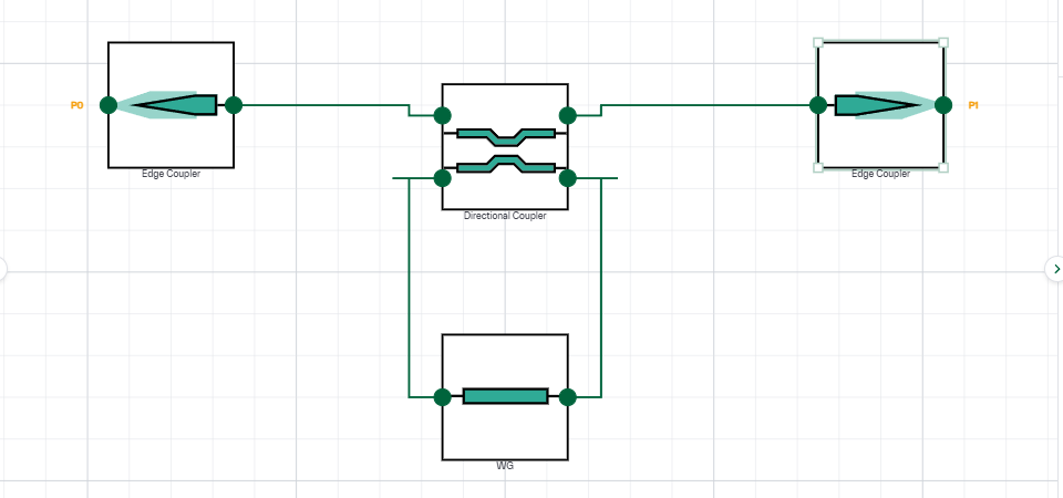
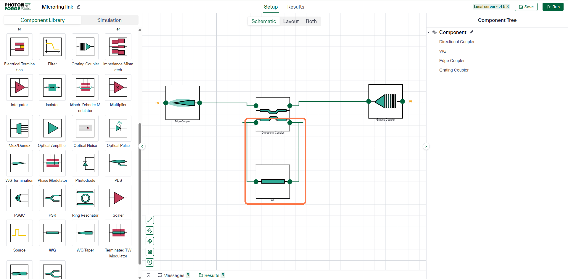
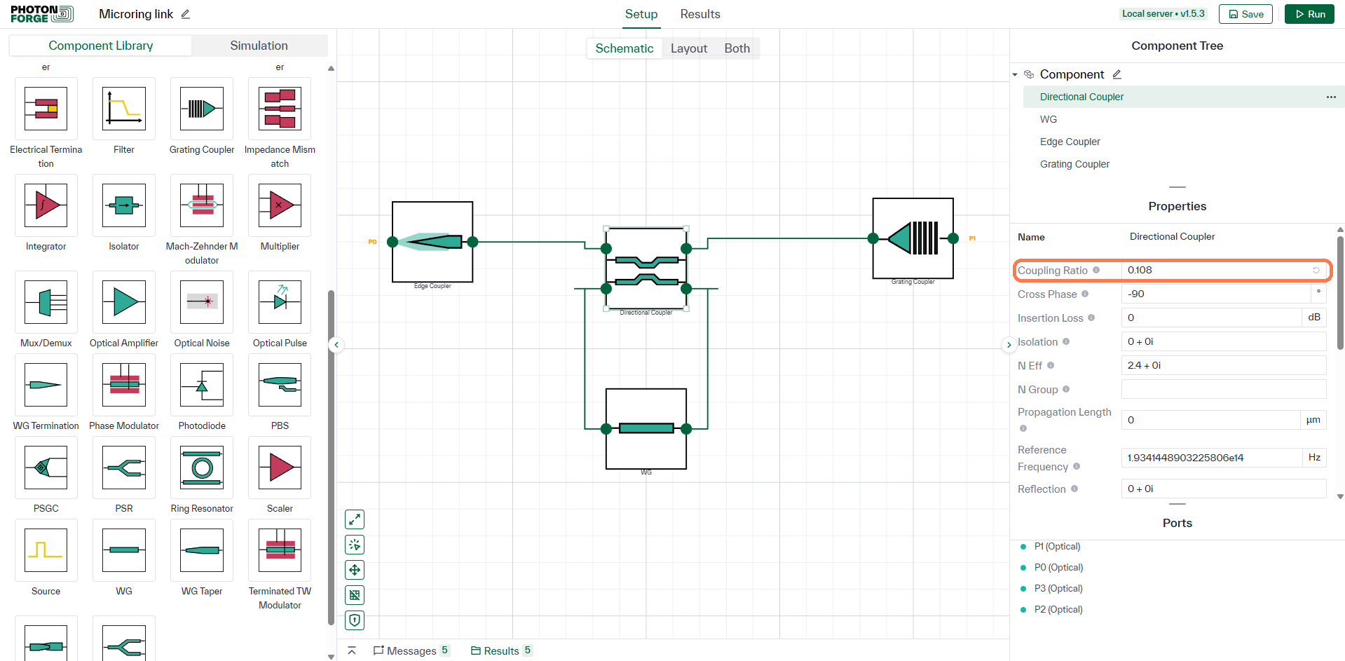
Drop a Directional Coupler on the canvas and run the bus straight through it: P0 in, P2 out. Then close the loop by wiring P3 back to P1 through a WG. Light that crosses into the loop travels once around and re‑enters the coupler, and that feedback is the whole resonator. An Edge Coupler and a Grating Coupler at each end bring light on and off the chip.
Sanity check: the loop is the one connection that is easy to get wrong. If your spectrum comes out flat with no dips at all, the loop wire did not take.
How much light survives a lap
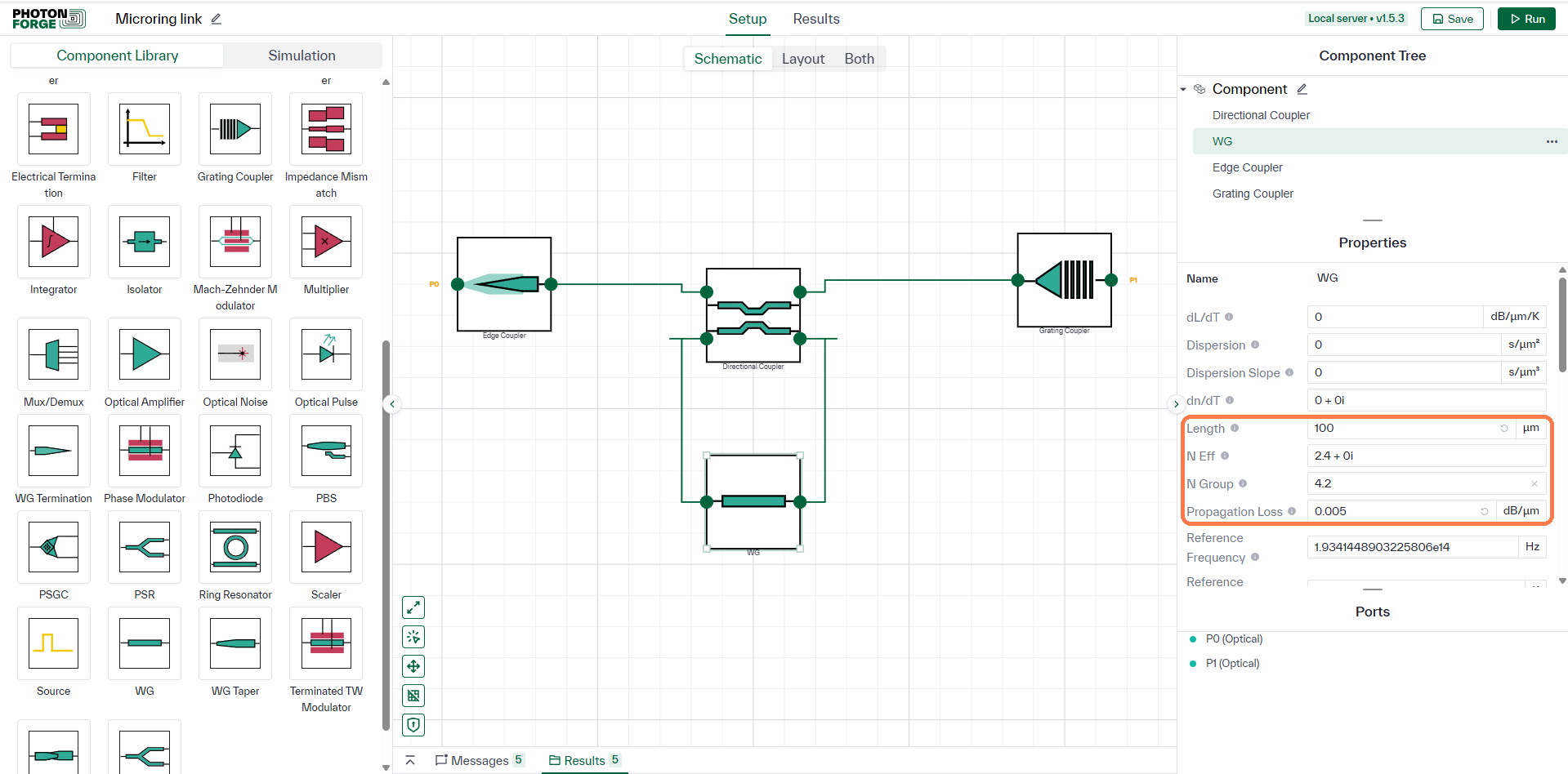
The loop waveguide sets the round trip: Length 100 µm, N Eff 2.4, N Group 4.2 and Propagation Loss 0.005 dB/µm. Two numbers follow. A lap costs 0.5 dB, so the fraction of amplitude that makes it back around is a ≈ 0.9441; and the length and group index together fix how far apart the resonances land.

Tip: if N Group is left blank it falls back to N Eff. Setting it to 4.2 here is what makes the resonance spacing realistic for silicon.
Matching the coupler to the loss
The Coupling Ratio κ is the fraction of power that crosses into the loop on each pass, so the amplitude staying in the bus is √(1 − κ). The resonance goes deepest when the light leaking back out of the ring exactly cancels the light that never entered it, and that happens when those two amplitudes are equal. The loss we just set therefore picks κ for us:

We will use Coupling Ratio = 0.108. At exact critical coupling the cancellation is perfect and the transmission at resonance is zero; at 0.108 roughly one part in 105 of the input power gets through. Both are far below anything you would measure, which is a good reminder that decibels exaggerate the gap between numbers that are effectively zero.
Two ways to reach the chip
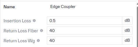
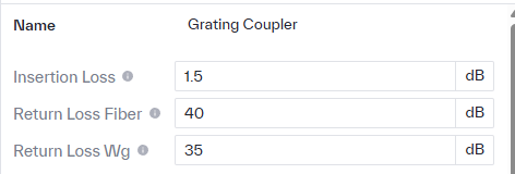
Both couplers take an insertion loss and two return losses, and on both, P0 is the fiber side and P1 the waveguide side. The defaults capture the real trade‑off: an edge coupler is far more efficient, while a grating coupler costs about a decibel more but can be probed anywhere on the wafer without dicing a facet. Together they put 2 dB in front of the ring before it does anything.
Enough points to see the resonance
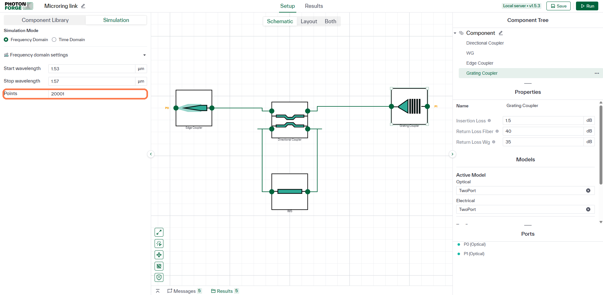
Sweep 1.53 to 1.57 µm with 20001 points. That sounds excessive for a 40 nm span until you notice the resonances are only about 0.2 nm wide: a coarse grid steps straight over the bottom of the dip and reports a resonance tens of decibels shallower than it really is. Analytical models are cheap, so resolution costs you seconds.
Seven resonances on a 2 dB floor
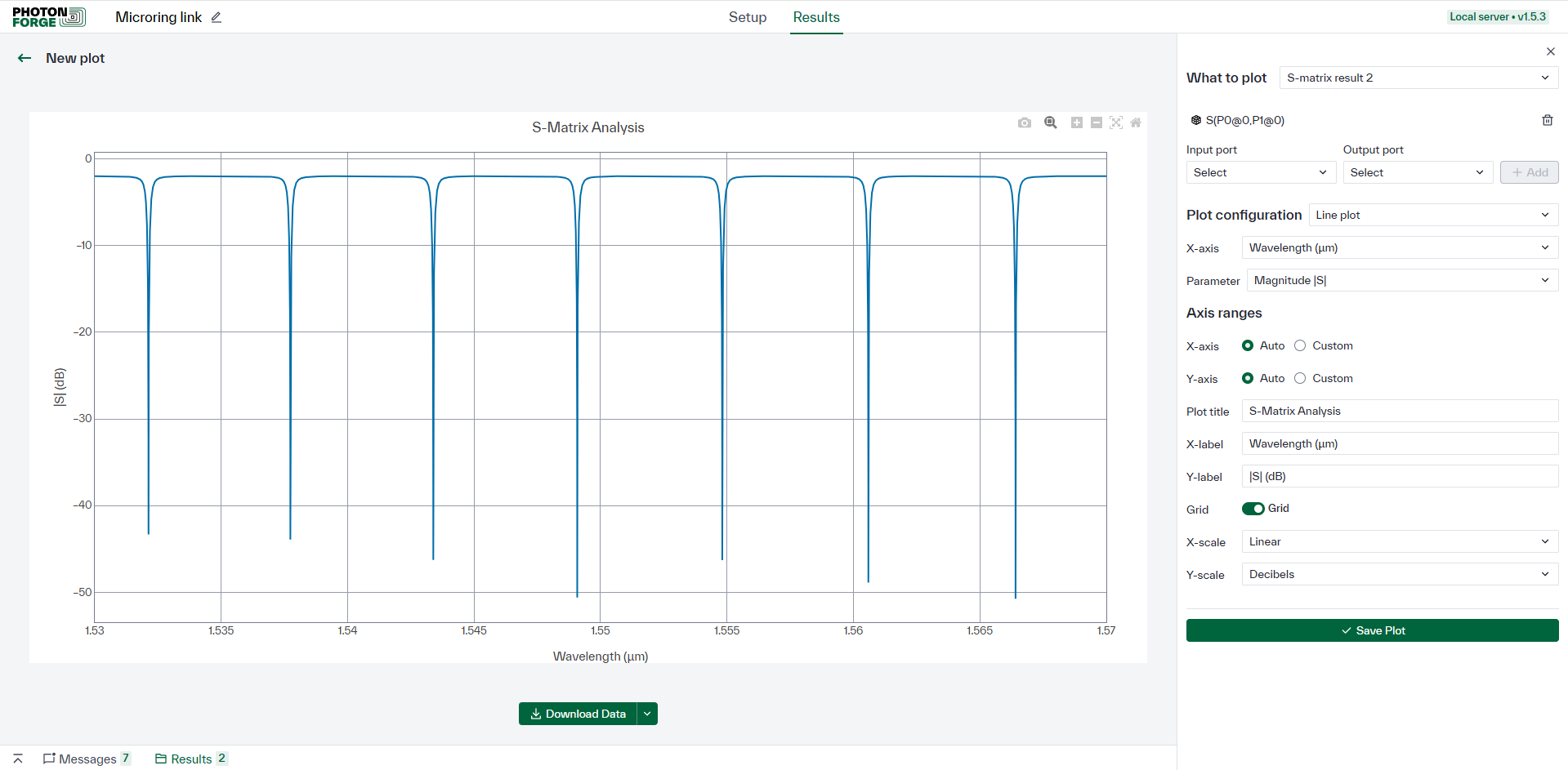
Run, then plot S between the two fiber ports. Two things are worth reading off this plot. The baseline sits at −2 dB, which is exactly the 0.5 plus 1.5 of the two fiber interfaces: off resonance, the ring is invisible and you are looking at your I/O budget. And the seven dips are spaced 5.7 nm apart, matching the FSR we predicted from the loop length and group index.
Where the light goes to die
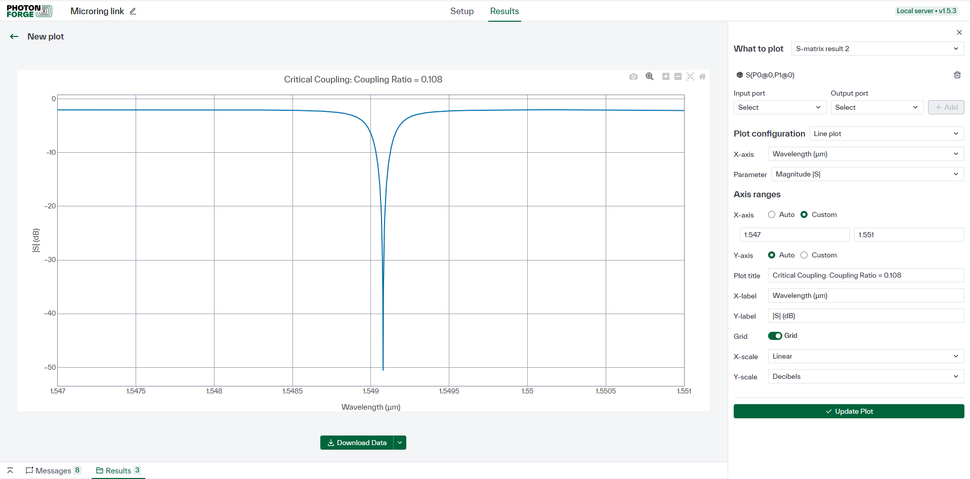
Set the X‑axis to Custom, 1.547 to 1.551 to zoom in on one resonance, and it plunges past −50 dB. This is the payoff of the κ = 0.108 we worked out in step 3: the two amplitudes really do cancel, and almost nothing reaches the output. The ring is critically coupled, and a null this deep is the most sensitive feature a resonator gives you.
Change one number, lose the null
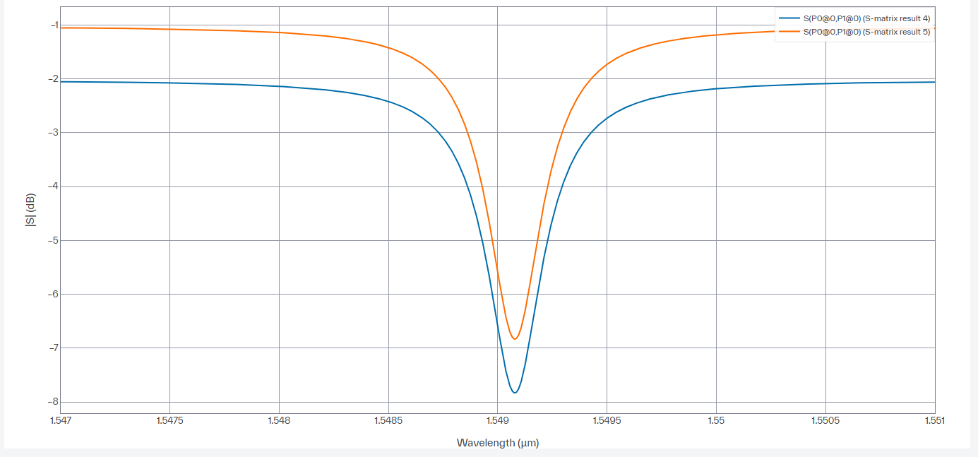
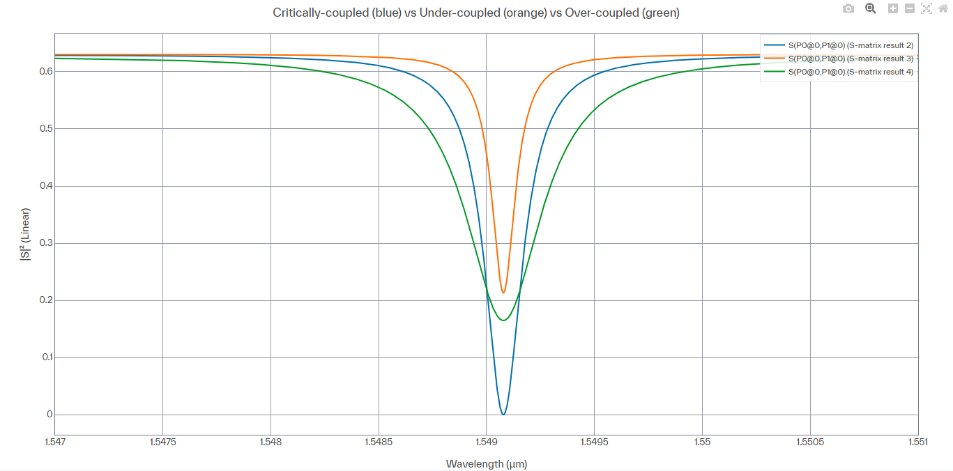
Change only the Coupling Ratio and re‑run, saving each plot. Let too little light in (0.03) and the ring cannot cancel the bus; let too much in (0.30) and it overshoots. Either way the cancellation stops being exact and the null collapses from more than 50 dB to under 8.

The width gives away which side you are on
Under‑coupled and over‑coupled reach nearly the same depth, −6.7 against −7.8 dB, so depth alone will not tell you which one a measured ring is. The linewidth will. Plot all three together as transmitted power on a linear scale and the difference is obvious: letting less light in per lap keeps photons circulating longer, so the under‑coupled resonance is the sharpest and the over‑coupled one is three times broader. Only the critical curve reaches zero.
One axis, three runs. Each coupling ratio produced its own S‑matrix result, and the plot editor lets you add traces from different results to the same plot: pick a result under What to plot, add the S‑parameter you want, then switch the result and add the next one. Overlaying runs this way is far easier to read than comparing separate plots side by side.

The budget moves, the physics does not
Replace the grating coupler with a second edge coupler and run again. Plotting both results together, the baseline lifts from −2 dB to −1 dB, the decibel you just saved, while the resonance keeps its shape and position. Your fiber interfaces and your resonator are independent parts of the budget, and this is how you separate them.