





import matplotlib.pyplot as plt
import numpy as np
import tidy3d as td
import tidy3d.web as web
from tidy3d.plugins.dispersion import FastDispersionFitter
TIDY3D
LEARNING CENTER
Example Library

Metasurface hologram
Note: running this notebook end to end submits cloud simulations and costs approximately 20 FlexCredits, dominated by the full \(128 \times 128\) FDTD run.
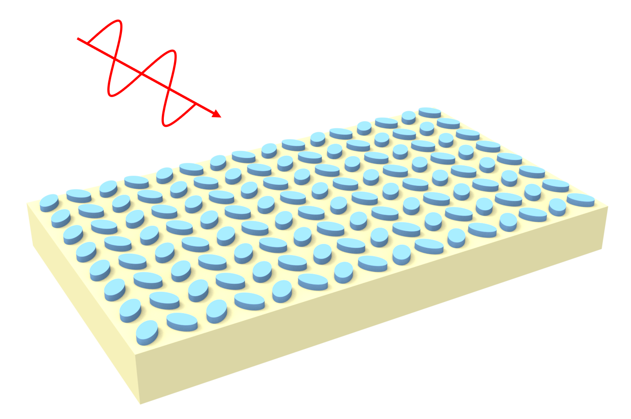
Geometric-phase (Pancharatnam-Berry) metasurfaces shape a wavefront by rotating subwavelength nanostructures rather than by changing their size. A birefringent nanofin that behaves as a half-wave plate, rotated in-plane by an angle \(\theta\), imprints a geometric phase of \(2\theta\) on the cross-circularly-polarized light it transmits. Assigning a rotation angle to each fin therefore lets an array synthesize an arbitrary phase profile — including one whose far field reconstructs a target image.
In this notebook, we design such a hologram end to end and reconstruct its projected field with a single full-device FDTD simulation. We use the amorphous-TiO\(_2\) nanofin platform of R. C. Devlin, M. Khorasaninejad, W. T. Chen, J. Oh, and F. Capasso, “Broadband high-efficiency dielectric metasurfaces for the visible spectrum,” Proc. Natl. Acad. Sci. USA 113, 10473-10478 (2016) at a design wavelength of \(532\) nm, and target the Mona Lisa as the projected image. The full \(128 \times 128\) surface concentrates roughly 90% of the transmitted power into a recognizable reconstruction.
The workflow has three steps:
- Unit cell — characterize a single nanofin: its circular polarization-conversion efficiency and the linear geometric phase \(\arg(t_\mathrm{conv}) = 2\theta\).
- Hologram design — retrieve the aperture phase map with the Gerchberg-Saxton algorithm.
- Full surface — build the finite array, run one FDTD simulation, and reconstruct the far field.
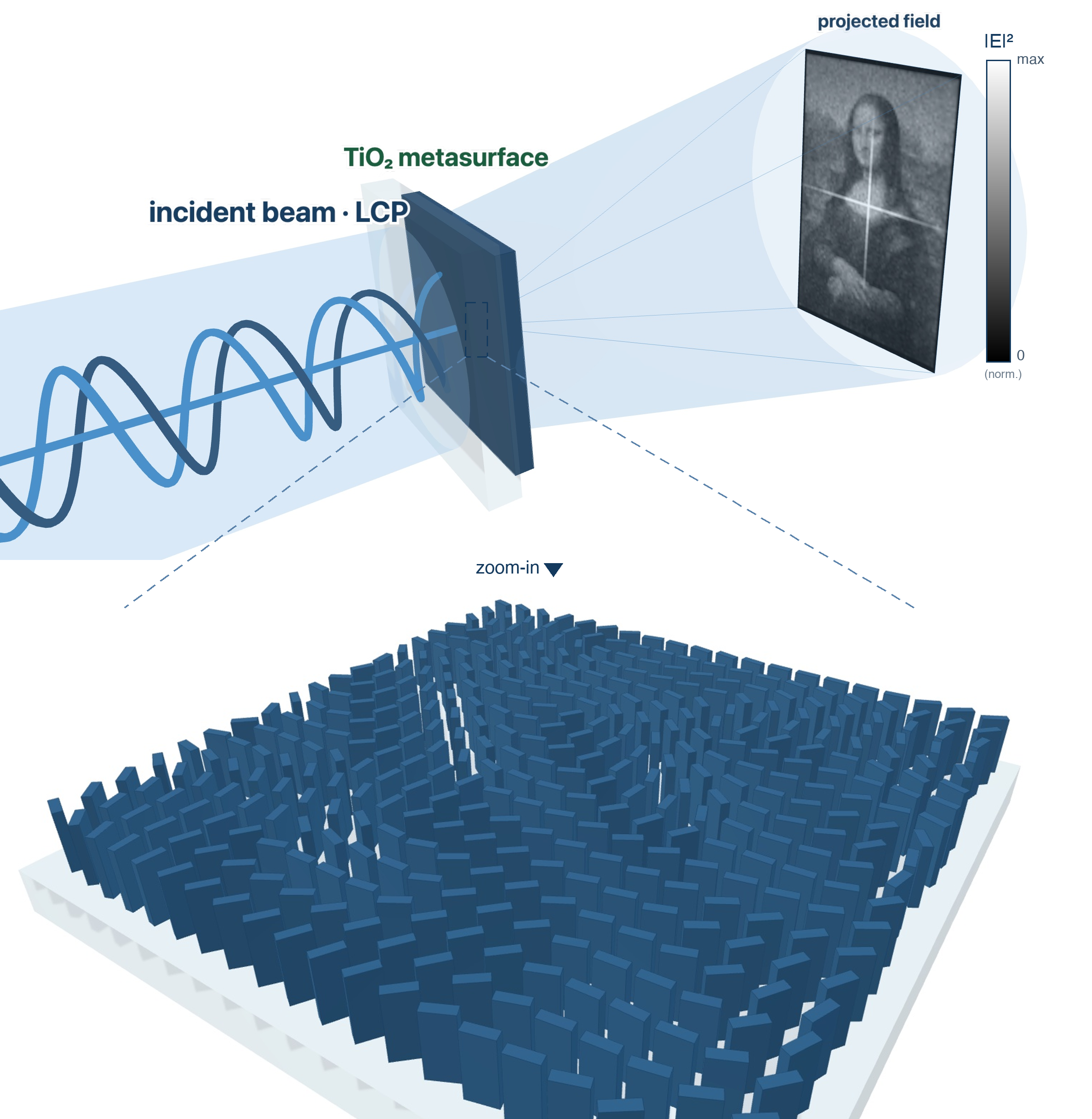
For more metasurface and diffractive-optics examples, please visit our examples page. If you are new to the finite-difference time-domain (FDTD) method, we highly recommend going through our FDTD101 tutorials.
Simulation Setup
We work in microns and set the design wavelength and central frequency. The nanofin dimensions (length L, width W, height H) and the unit-cell pitch S are the \(532\) nm design of Devlin et al. The full surface is N by N fins; here N = 128 (a 41.6 µm aperture) resolves a clearly legible far-field reconstruction.
lda0 = 0.532                 # design wavelength (um)
freq0 = td.C_0 / lda0        # design frequency
L, W, H = 0.25, 0.085, 0.6   # nanofin length, width, height (um)
S = 0.325                    # unit-cell pitch (um)
N = 128                      # full-surface array size (fins per side)
sign = +1                    # geometric-phase sign (calibrated so the image lands at +u)

# hologram / far-field design parameters
u_center = (0.0, 0.0)        # image centered on-axis (direction cosines)
u_width = 0.48               # image width in direction cosines
u_win = 0.70                 # far-field projection half-window
gs_iters = 400               # Gerchberg-Saxton iterations
margin = 0.65                # bare-glass margin around the aperture (um)
The nanofins are amorphous TiO\(_2\) on a fused-silica substrate. We fit a lossless dispersive model to refractive-index data digitized from Fig. 1A of Devlin et al. using the FastDispersionFitter.
tio2_nk = np.array(
    [(0.400, 2.63), (0.420, 2.57), (0.440, 2.52), (0.460, 2.49), (0.480, 2.46),
     (0.500, 2.43), (0.532, 2.42), (0.560, 2.40), (0.600, 2.385), (0.640, 2.37),
     (0.660, 2.365), (0.700, 2.355), (0.750, 2.34), (0.800, 2.33)]
)
fitter = FastDispersionFitter(
    wvl_um=tio2_nk[:, 0], n_data=tio2_nk[:, 1], k_data=np.zeros(len(tio2_nk))
)
tio2, rms = fitter.fit(max_num_poles=3, tolerance_rms=2e-3)
print(f"TiO2 dispersion fit RMS = {rms:.2e}")

sio2 = td.Medium(permittivity=1.46**2)   # fused silica (nearly dispersionless here)
TiO2 dispersion fit RMS = 6.80e-041. Unit Cell
A single nanofin behaves as a half-wave plate when the phase retardance between its long and short axes reaches \(180\) degrees. We verify this by running two PlaneWave simulations of the periodic cell with the field polarized along the fin length and along its width, then reading the complex zero-order transmission from a DiffractionMonitor. The converted (cross-circular) efficiency is \(\eta_\mathrm{conv} = |t_L - t_W|^2 / 4\). A rotation sweep then confirms the geometric phase \(\arg(t_\mathrm{conv}) = 2\theta\).
The make_unit_cell helper builds one periodic cell. The periodic fin array supports high-Q guided-mode resonances that ring long after the pulse, so we apodize the DFT time window to avoid spectral ripple.
uc_ldas = np.linspace(0.46, 0.70, 81)
uc_freqs = np.sort(np.unique(np.concatenate([td.C_0 / uc_ldas, [freq0]])))
uc_freq0 = 0.5 * (uc_freqs.min() + uc_freqs.max())
uc_fwidth = 0.5 * (uc_freqs.max() - uc_freqs.min())
thetas = np.arange(8) * np.pi / 8   # rotation sweep, 0 to 157.5 deg


def make_unit_cell(pol_angle: float, theta: float = 0.0, with_fin: bool = True) -> td.Simulation:
    """Periodic TiO2 nanofin unit cell, plane wave incident from the glass side."""
    structures = [td.Structure(
        geometry=td.Box.from_bounds(rmin=(-td.inf, -td.inf, -1.6), rmax=(td.inf, td.inf, 0)),
        medium=sio2)]
    if with_fin:
        fin = td.Box(center=(0, 0, 0), size=(L, W, H))
        fin_arr = fin.array(offsets=[(0, 0, H / 2)],
                            transforms=[td.Transformed.rotation(theta, axis=2)])
        structures.append(td.Structure(geometry=fin_arr, medium=tio2))
    plane_wave = td.PlaneWave(
        source_time=td.GaussianPulse(freq0=uc_freq0, fwidth=uc_fwidth),
        size=(td.inf, td.inf, 0), center=(0, 0, -0.5), direction="+", pol_angle=pol_angle)
    diff_mnt = td.DiffractionMonitor(
        center=(0, 0, 1.0), size=(td.inf, td.inf, 0), freqs=list(uc_freqs), name="diff",
        normal_dir="+", apodization=td.ApodizationSpec(end=0.6e-12, width=0.1e-12))
    return td.Simulation(
        center=(0, 0, 0.3), size=(S, S, 2.2),
        structures=structures, sources=[plane_wave], monitors=[diff_mnt], run_time=1.5e-12,
        boundary_spec=td.BoundarySpec(
            x=td.Boundary.periodic(), y=td.Boundary.periodic(), z=td.Boundary.pml()),
        grid_spec=td.GridSpec.auto(min_steps_per_wvl=30, wavelength=0.46),
        medium=td.Medium(permittivity=1.0))
We assemble the batch: the two linear polarizations, a fin-free reference for the aperture normalization, and the rotation sweep. Before running, we visualize one cell to confirm the fin sits on the substrate and the source and monitor are placed correctly.
sims = {"polL": make_unit_cell(0.0), "polW": make_unit_cell(np.pi / 2),
        "ref": make_unit_cell(0.0, with_fin=False)}
for i, th in enumerate(thetas):
    sims[f"rot_{i}"] = make_unit_cell(0.0, theta=th)

fig, (ax1, ax2) = plt.subplots(1, 2, figsize=(10, 4), tight_layout=True)
sims["polL"].plot(y=0, ax=ax1)
sims["polL"].plot(z=H / 2, ax=ax2)
plt.show()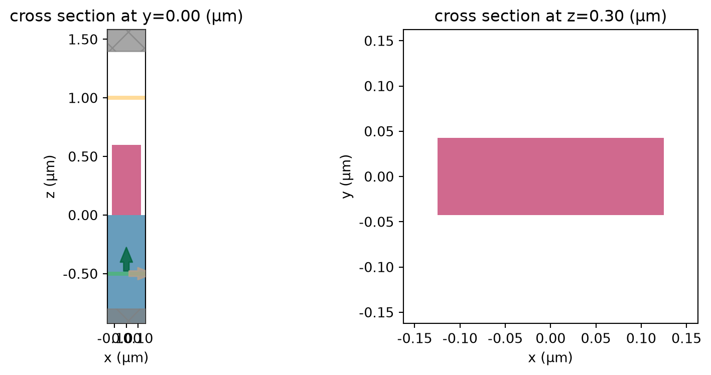
We estimate the batch cost before submitting. The reported value is the maximum FlexCredit cost; each run auto-shuts-off once the field decays, so we are billed only for the effective run time.
batch = web.Batch(simulations=sims, folder_name="metasurface_hologram")
batch.estimate_cost()
05:27:53 UTC Maximum FlexCredit cost: 0.300 for the whole batch.
0.2995031950966639batch_data = batch.run(path_dir="data")05:27:54 UTC Started working on Batch containing 11 tasks.
05:28:04 UTC Maximum FlexCredit cost: 0.300 for the whole batch.
             Use 'Batch.real_cost()' to get the billed FlexCredit cost after
             completion.
05:28:11 UTC Batch complete.
Postprocessing
We read the complex zero-order amplitudes ("p" is Ex-like, "s" is Ey-like) and compute the conversion efficiency spectrum and the retardance at the design wavelength.
def zero_order(sim_data):
    """Complex zero-order (p, s) transmission amplitudes vs frequency."""
    amps = sim_data["diff"].amps.sel(orders_x=0, orders_y=0)
    return amps.sel(polarization="p").values, amps.sel(polarization="s").values


lam = td.C_0 / uc_freqs
i0 = np.argmin(np.abs(lam - lda0))
T_ref = np.abs(zero_order(batch_data["ref"])[0]) ** 2
tL = zero_order(batch_data["polL"])[0]
tW = zero_order(batch_data["polW"])[1]
eta_conv = np.abs(tL - tW) ** 2 / 4
retardance = np.degrees(np.angle(tL[i0] / tW[i0]))
print(f"conversion efficiency at {lda0 * 1e3:.0f} nm = "
      f"{100 * eta_conv[i0] / T_ref[i0]:.1f}% (aperture-normalized)")
print(f"retardance = {retardance:.0f} deg (target 180)")
conversion efficiency at 532 nm = 97.7% (aperture-normalized)
retardance = 161 deg (target 180)To extract the geometric phase, we isolate the converted amplitude \(t_\mathrm{conv}(\theta)\) from the circular components of the transmitted zero order at each rotation angle, and fit its phase against \(\theta\).
t_conv = []
for i, th in enumerate(thetas):
    p, s = zero_order(batch_data[f"rot_{i}"])
    a_plus = (p[i0] - 1j * s[i0]) / np.sqrt(2)   # sigma+ output content
    a_minus = (p[i0] + 1j * s[i0]) / np.sqrt(2)  # sigma- output content
    if abs(np.sin(2 * th)) > 1e-3:
        t_conv.append((a_minus - a_plus) / (2j * np.sin(2 * th)) * np.sqrt(2))
    else:
        t_conv.append((tL[i0] - tW[i0]) / 2)
t_conv = np.array(t_conv)
phase = 2 * thetas + np.angle(t_conv * np.conj(t_conv[0]))
slope = np.polyfit(thetas, phase, 1)[0]
print(f"geometric-phase slope d(phase)/d(theta) = {slope:.3f} (expect +2.000)")
geometric-phase slope d(phase)/d(theta) = 2.002 (expect +2.000)fig, (ax1, ax2) = plt.subplots(1, 2, figsize=(11, 4), tight_layout=True)
ax1.plot(lam * 1e3, 100 * eta_conv / T_ref, lw=2)
ax1.axvline(lda0 * 1e3, color="k", ls="--", lw=0.8)
ax1.set_xlabel(r"Wavelength (nm)")
ax1.set_ylabel("Conversion efficiency (%)")
ax1.set_xlim(460, 700)
ax1.set_ylim(0, 100)
ax1.grid(alpha=0.3)
ax2.plot(np.degrees(thetas), np.degrees(phase), "o-", label="converted phase")
ax2.plot(np.degrees(thetas), np.degrees(2 * thetas), "k--", lw=1, label=r"ideal $2\theta$")
ax2.set_xlabel(r"Fin rotation $\theta$ (deg)")
ax2.set_ylabel("Converted phase (deg)")
ax2.legend()
ax2.grid(alpha=0.3)
plt.show()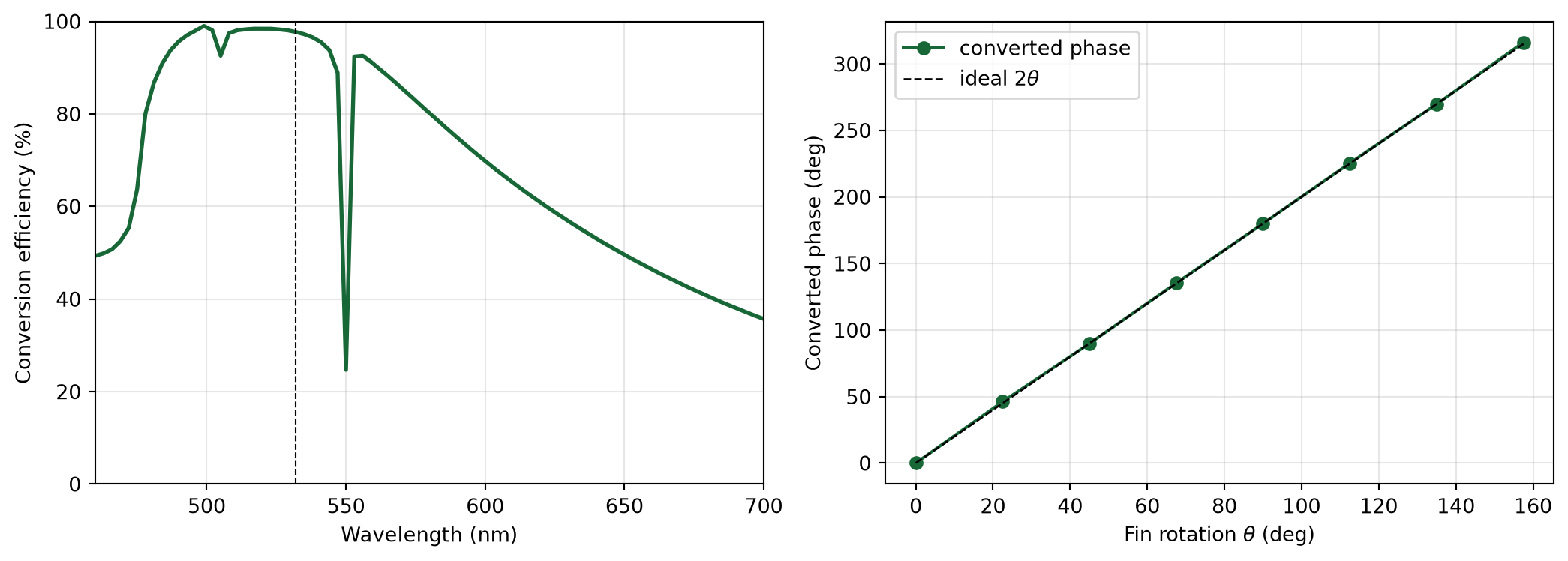
The fin reaches near-\(180\) degree retardance with high conversion efficiency at \(532\) nm, and the converted phase tracks the ideal \(2\theta\) line — so a rotation map directly encodes a phase map.
2. Hologram Design
The far field of the aperture is the Fourier transform of its transmitted field. Because the metasurface is phase-only (unit amplitude), we recover the required aperture phase with the Gerchberg-Saxton algorithm: it alternates between the aperture plane (enforce unit amplitude) and the far-field plane (enforce the target amplitude). We load a public-domain scan of the Mona Lisa (bundled with the notebook in misc/) and place it, at the array’s native resolution, on the direction-cosine grid.
def resize_gray(a, w, h):
    """Area-average (box) downsample of a 2D array to shape (h, w)."""
    yb = np.linspace(0, a.shape[0], h + 1).astype(int)
    xb = np.linspace(0, a.shape[1], w + 1).astype(int)
    return np.array([[a[yb[i]:yb[i + 1], xb[j]:xb[j + 1]].mean()
                      for j in range(w)] for i in range(h)])


def dilate(mask, iters=2):
    """Binary dilation with a 4-connected structuring element."""
    m = mask.copy()
    for _ in range(iters):
        d = m.copy()
        d[1:, :] |= m[:-1, :]
        d[:-1, :] |= m[1:, :]
        d[:, 1:] |= m[:, :-1]
        d[:, :-1] |= m[:, 1:]
        m = d
    return m


def make_target(n: int):
    """Grayscale-intensity target on the n-by-n k-space grid, indexed [ix, iy] with y up."""
    rows = plt.imread("misc/mona_lisa.jpg")[..., :3].mean(axis=2) / 255   # grayscale in [0, 1]
    h_px, w_px = rows.shape
    du = lda0 / (n * S)
    w_bins = int(round(u_width / du))
    h_bins = int(round(u_width * h_px / w_px / du))
    small = resize_gray(rows, w_bins, h_bins)
    img_xy = np.flipud(small).T
    target = np.zeros((n, n))
    u = (np.arange(n) - n // 2) * du
    ic = np.argmin(np.abs(u - u_center[0]))
    jc = np.argmin(np.abs(u - u_center[1]))
    i0, j0 = ic - w_bins // 2, jc - h_bins // 2
    target[i0:i0 + w_bins, j0:j0 + h_bins] = np.clip(img_xy, 0, 1)
    ux, uy = np.meshgrid(u, u, indexing="ij")
    target[ux**2 + uy**2 >= 1] = 0     # drop non-propagating (evanescent) bins
    return target, u


def gerchberg_saxton(target, n_iter: int = gs_iters):
    """Classic Gerchberg-Saxton; returns phase-only aperture phase phi[ix, iy]."""
    amp_t = np.sqrt(target)
    amp_t /= np.linalg.norm(amp_t)
    rng = np.random.default_rng(7)
    field = amp_t * np.exp(2j * np.pi * rng.random(target.shape))
    aperture = None
    for _ in range(n_iter):
        aperture = np.fft.fftshift(np.fft.ifft2(np.fft.ifftshift(field)))
        aperture = np.exp(1j * np.angle(aperture))          # aperture: phase only
        field = np.fft.fftshift(np.fft.fft2(np.fft.ifftshift(aperture)))
        field = amp_t * np.exp(1j * np.angle(field))        # far field: target amplitude
    return np.angle(aperture)


target, u = make_target(N)
phi = gerchberg_saxton(target)
We check the design by taking the far field of the retrieved phase map and measuring the fraction of power that lands in the image.
I_pred = np.abs(np.fft.fftshift(np.fft.fft2(np.fft.ifftshift(np.exp(1j * phi))))) ** 2
window = dilate(target > 0.05, 2)
print(f"predicted power in image window = {100 * I_pred[window].sum() / I_pred.sum():.0f}%")

fig, axes = plt.subplots(1, 3, figsize=(13, 4.2), tight_layout=True)
ext_u = [u[0], u[-1], u[0], u[-1]]
axes[0].imshow(target.T, origin="lower", extent=ext_u, cmap="gray")
axes[0].set_title("target")
axes[1].imshow(phi.T, origin="lower", cmap="twilight",
               extent=[-N * S / 2, N * S / 2, -N * S / 2, N * S / 2])
axes[1].set_title(r"aperture phase $\phi(x, y)$")
axes[2].imshow(I_pred.T, origin="lower", extent=ext_u, cmap="gray",
               vmax=np.percentile(I_pred, 99.7))
axes[2].set_title("predicted reconstruction")
for ax in (axes[0], axes[2]):
    ax.set_xlabel(r"$u_x$")
    ax.set_ylabel(r"$u_y$")
axes[1].set_xlabel(r"x ($\mu m$)")
plt.show()
predicted power in image window = 96%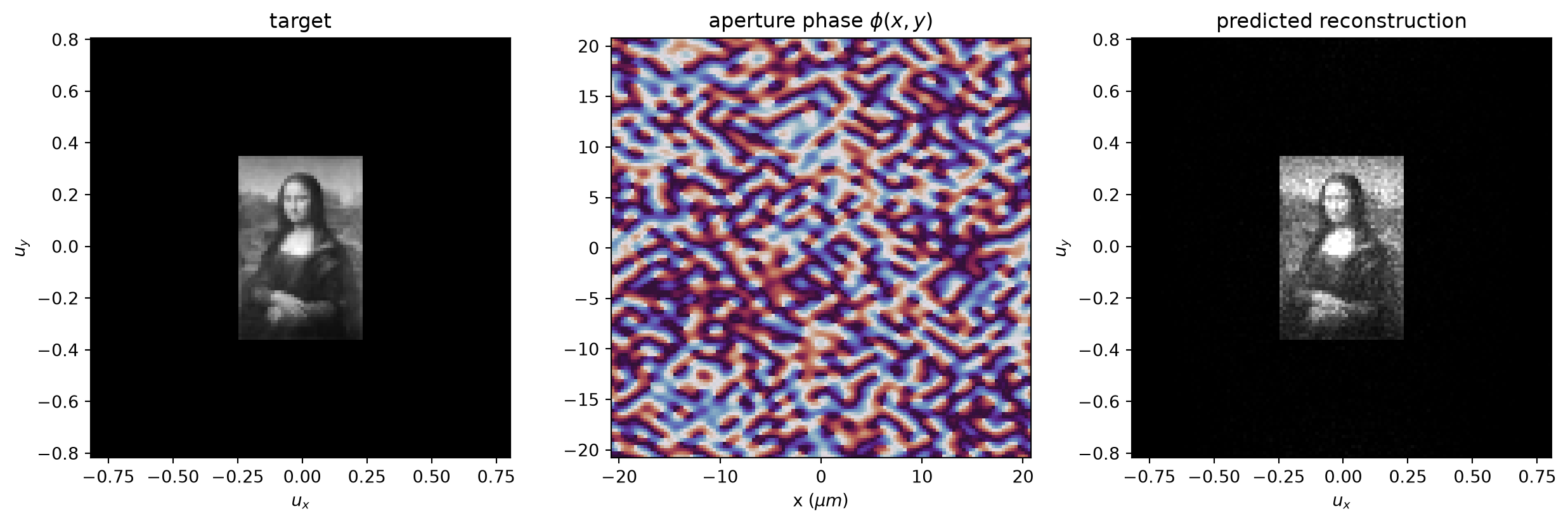
3. Full Surface
Now we build the finite metasurface: fin \(i\) is a rotated rectangular PolySlab at angle \(\theta_i = \mathrm{sign}\cdot\phi_i/2\), all collected in a GeometryGroup. We illuminate from the glass side with circularly polarized light — two overlapping plane waves with the \(y\) component delayed by \(\pi/2\) — and record the far field with a FieldProjectionKSpaceMonitor plus a FluxMonitor for the transmitted power.
def make_full_sim(n: int, phi: np.ndarray) -> td.Simulation:
    """Finite n-by-n rotated-nanofin metasurface with circularly polarized illumination."""
    thetas = (sign * phi / 2).ravel()
    aperture = n * S
    size_xy = aperture + 2 * margin

    coords = (np.arange(n) - n / 2 + 0.5) * S
    xs, ys = np.meshgrid(coords, coords, indexing="ij")
    xs, ys = xs.ravel(), ys.ravel()
    v0 = np.array([[+L / 2, +W / 2], [-L / 2, +W / 2], [-L / 2, -W / 2], [+L / 2, -W / 2]])
    rot = np.array([[np.cos(thetas), -np.sin(thetas)], [np.sin(thetas), np.cos(thetas)]])
    verts = np.einsum("ij,jkn->nik", v0, rot) + np.stack([xs, ys], axis=-1)[:, None, :]
    fins = td.Structure(
        geometry=td.GeometryGroup(geometries=[
            td.PolySlab(vertices=v.tolist(), slab_bounds=(0, H), axis=2) for v in verts]),
        medium=tio2)
    substrate = td.Structure(
        geometry=td.Box.from_bounds(rmin=(-td.inf, -td.inf, -1.5), rmax=(td.inf, td.inf, 0)),
        medium=sio2)

    pulse_x = td.GaussianPulse(freq0=freq0, fwidth=freq0 / 10, phase=0)
    pulse_y = td.GaussianPulse(freq0=freq0, fwidth=freq0 / 10, phase=-np.pi / 2)
    src_x = td.PlaneWave(source_time=pulse_x, size=(td.inf, td.inf, 0), center=(0, 0, -0.4),
                         direction="+", pol_angle=0)
    src_y = src_x.updated_copy(source_time=pulse_y, pol_angle=np.pi / 2)

    du = lda0 / aperture
    n_half = int(u_win / du)
    u_pts = list(np.arange(-n_half, n_half + 1) * du)
    apod = td.ApodizationSpec(end=0.5e-12, width=0.08e-12)
    kspace_mnt = td.FieldProjectionKSpaceMonitor(
        center=(0, 0, 0.8), size=(td.inf, td.inf, 0), freqs=[freq0], name="kspace",
        proj_axis=2, ux=u_pts, uy=u_pts, apodization=apod)
    flux_mnt = td.FluxMonitor(center=(0, 0, 0.8), size=(td.inf, td.inf, 0), freqs=[freq0],
                              name="flux", apodization=apod)

    # uniform in-plane grid resolves every fin identically; AutoGrid in z refines
    # inside the high-index TiO2 automatically (no override structure needed)
    grid_xy = td.UniformGrid(dl=S / 20)
    grid_spec = td.GridSpec(
        wavelength=lda0, grid_x=grid_xy, grid_y=grid_xy,
        grid_z=td.AutoGrid(min_steps_per_wvl=20))
    return td.Simulation(
        center=(0, 0, 0.25), size=(size_xy, size_xy, 2.0),
        structures=[substrate, fins], sources=[src_x, src_y],
        monitors=[kspace_mnt, flux_mnt], run_time=1.5e-12,
        boundary_spec=td.BoundarySpec(
            x=td.Boundary.absorber(), y=td.Boundary.absorber(), z=td.Boundary.pml()),
        grid_spec=grid_spec, medium=td.Medium(permittivity=1.0))


sim = make_full_sim(N, phi)
Before running, we visualize the setup: a side view of the substrate, fins, and source, and a zoomed top view showing the individual rotated fins.
fig, (ax1, ax2) = plt.subplots(1, 2, figsize=(12, 5), tight_layout=True)
sim.plot(x=0, ax=ax1)
sim.plot(z=H / 2, ax=ax2)
ax2.set_xlim(-2, 2)
ax2.set_ylim(-2, 2)
plt.show()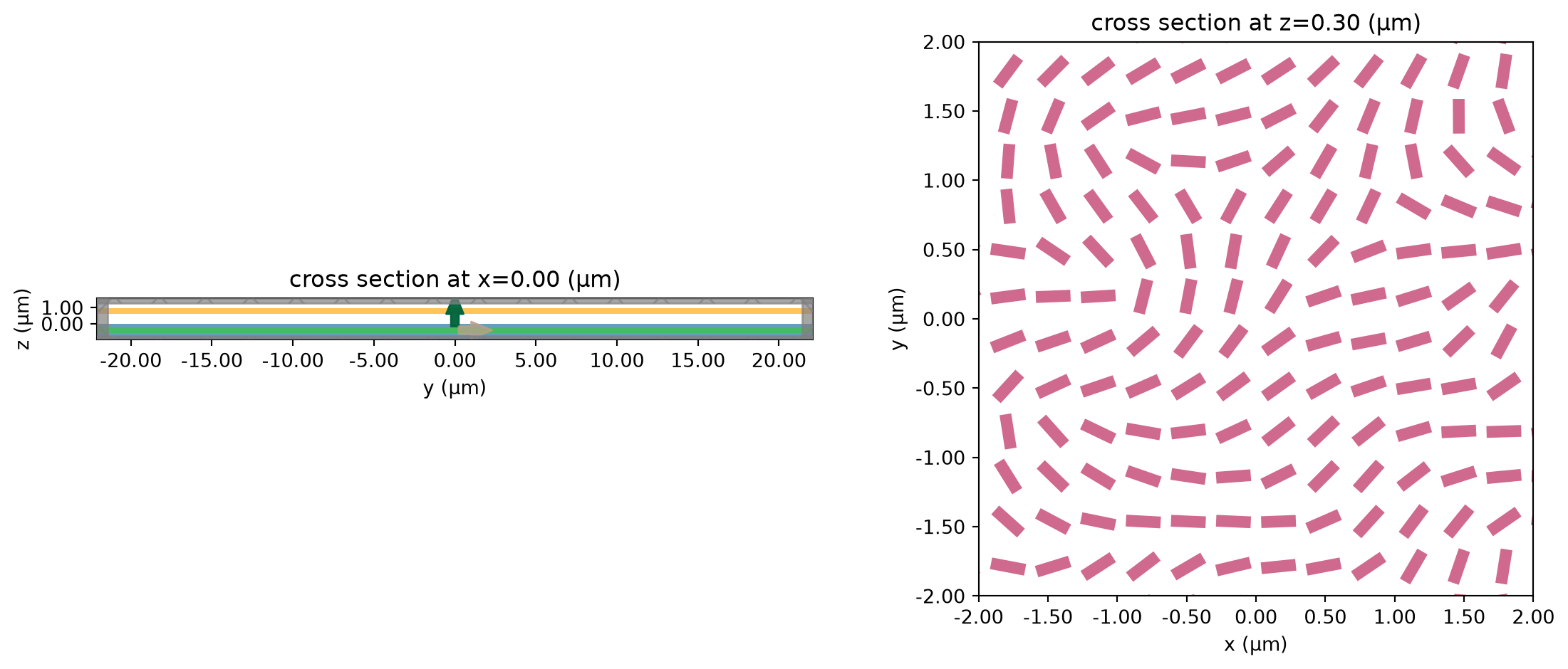
We estimate the cost, then submit the single full-device simulation.
job = web.Job(simulation=sim, task_name="metasurface_hologram_full", folder_name="metasurface_hologram")
cost = web.estimate_cost(job.task_id)
05:28:27 UTC Created task 'metasurface_hologram_full' with resource_id 'fdve-293020bf-4a8b-44c4-afb7-1886bac2d3a3' and task_type 'FDTD'.
             View task using web UI at
             'https://tidy3d.simulation.cloud/workbench?taskId=fdve-293020bf-4a8
             b-44c4-afb7-1886bac2d3a3'.
Task folder: 'default'.
05:28:47 UTC Estimated FlexCredit cost: 19.598. This assumes the FDTD solver
             runs for the full simulation time; if early shutoff is reached, the
             billed cost can be lower. Use 'web.real_cost(task_id)' to get the
             billed FlexCredit cost after a simulation run.
sim_data = job.run(path="data/metasurface_hologram_full.hdf5")05:28:48 UTC status = success
05:28:49 UTC Loading results from data/metasurface_hologram_full.hdf5
Result Visualization
We integrate the projected far-field intensity with the direction-cosine solid-angle Jacobian, then measure the fraction of far-field power in the image window and the absolute conversion efficiency (image power divided by the power incident on the aperture). Because two orthogonal sources inject twice the reference power, the incident aperture power is \(2 A_\mathrm{ap} / A_\mathrm{dom}\).
kd = sim_data["kspace"]
Et = kd.fields_spherical.Etheta.squeeze(drop=True).transpose("ux", "uy")
Ep = kd.fields_spherical.Ephi.squeeze(drop=True).transpose("ux", "uy")
ux, uy = Et.ux.values, Et.uy.values
intensity = np.abs(Et.values) ** 2 + np.abs(Ep.values) ** 2
UX, UY = np.meshgrid(ux, uy, indexing="ij")
w2 = 1 - UX**2 - UY**2
P = intensity * np.where(w2 > 1e-6, 1 / np.sqrt(np.abs(w2)), 0.0)

iu = np.array([np.argmin(np.abs(u - v)) for v in ux])
tgt = target[np.ix_(iu, iu)]
signal = dilate(tgt > 0.05, 2)
frac_signal = P[signal].sum() / P.sum()

flux_t = sim_data["flux"].flux.values.item()
ap_frac = (N * S) ** 2 / sim.size[0] / sim.size[1]
eta_abs = frac_signal * flux_t / (2 * ap_frac)
print(f"far-field power in image window = {100 * frac_signal:.1f}%")
print(f"absolute efficiency (image / incident on aperture) = {100 * eta_abs:.1f}%")
far-field power in image window = 96.5%
absolute efficiency (image / incident on aperture) = 90.0%Finally, we compare the design target with the FDTD reconstruction. The bright cross at the center of the reconstruction is the residual on-axis zero order (un-converted co-polarized light) plus the square-aperture diffraction, a real feature of an on-axis hologram.
fig, (ax1, ax2) = plt.subplots(1, 2, figsize=(11, 5), tight_layout=True)
ext_u = [ux[0], ux[-1], ux[0], ux[-1]]
ax1.imshow(tgt.T, origin="lower", extent=ext_u, cmap="gray")
ax1.set_title("target")
ax2.imshow((P / P.max()).T, origin="lower", extent=ext_u, cmap="gray",
           vmax=np.percentile(P / P.max(), 99.7))
ax2.set_title(f"FDTD reconstruction (N = {N})")
for ax in (ax1, ax2):
    ax.set_xlabel(r"$u_x$")
    ax.set_ylabel(r"$u_y$")
plt.show()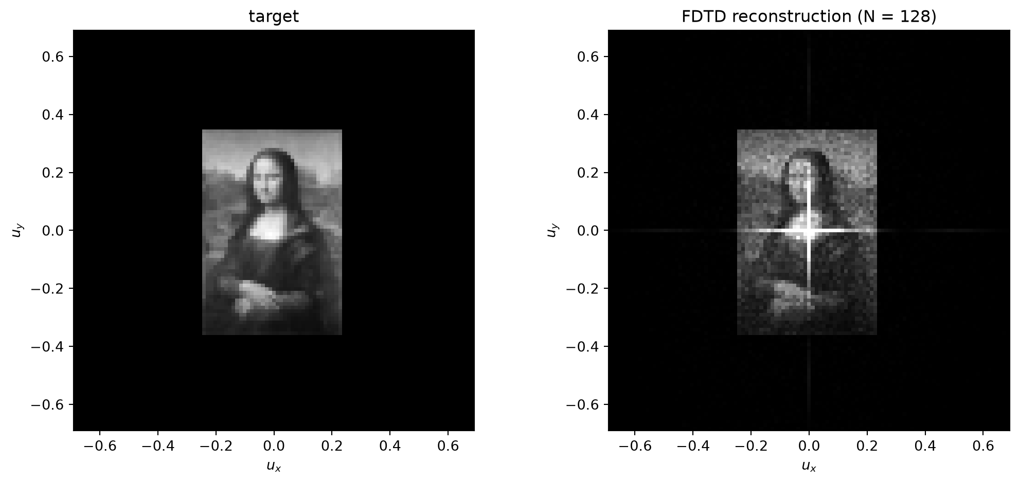
The finite metasurface reproduces the target in a single simulation, concentrating most of the transmitted power into a recognizable image. Increasing N (a larger aperture with more fins) sharpens the reconstruction at a proportionally higher simulation cost.


 TERMS & CONDITIONS


 How the process works:
 Try this real URL to see an example: