TIDY3D
LEARNING CENTER





Frequently Asked Questions
About Tidy3D
How is using Tidy3D billed?
The Tidy3D client that is used for designing simulations and analyzing the results is free and open source. A Tidy3D license is required to run simulations, either from FlexCredits (see What is a FlexCredit?) or from our virtual GPU option, which is a rented cluster dedicated to the customer. FlexCredits are based on the size of the simulation (in spatial size and physical simulation duration, as opposed to compute time). When a task is uploaded to our servers, we will print the maximum incurred cost in FlexCredit. This cost is also displayed in the online interface for that task. This value is determined by the cost associated with simulating the entire time stepping specified. This cost will be pro-rated if early shutoff is detected and the simulation is completed before the time stepping period. For more questions or to purchase FlexCredit, please contact us at support@flexcompute.com.
What is Tidy3D?
Can I get a discount as a student or teacher?
What are the advantages of Tidy3D compared to traditional EM simulators?
Do I have to know Python programming to use Tidy3D?
What is a FlexCredit?
FlexCredit is Flexcompute’s way of measuring computing power. It’s a unit we created to make it easier to understand and buy computing power.
A FlexCredit reflects the size of a simulation, in both grid points and timesteps. It does NOT reflect the compute time required to run the simulation, as Flexcompute’s compute time is always improving, and keeps us motivated to keep compute time as fast as possible.
However, to benchmark in more concrete terms for a new user, at the time of writing, one FlexCredit is roughly equivalent to about 50 hours of CPU core time when using the traditional FDTD method. That’s the equivalent of running a computer processor core for two days straight, just for one FlexCredit! If you have 60 FlexCredits, it’s like having a 4-core CPU (which is a pretty powerful computer) running non-stop, 24 hours a day, for a full month.
This makes it simple for our customers and employees. Instead of trying to communicate in terms of CPU hours or cores, they just need to know how many FlexCredits they need for their project. It’s like buying resources on a supercomputer but in a more straightforward, more understandable way.
How many CPU hours is one FlexCredit comparable to?
Note that FlexCredits reflect the spatial size and physical duration of a simulation, not its compute time. See What is a FlexCredit? for more details.
However, at the time of writing, one FlexCredit is roughly equivalent to about 50 hours of CPU core time when using the traditional FDTD method. That’s the equivalent of running a computer processor core for two days straight, just for one FlexCredit!
If you have 60 FlexCredits, it’s like having a 4-core CPU (which is a pretty powerful computer) running non-stop, 24 hours a day, for an entire month.
Does Tidy3D have a graphical user interface (GUI)?
Tidy3D comes with a feature-rich graphical user interface (GUI) that offers many tools to create and run electromagnetic simulations with ease and intuitiveness. With Tidy3D GUI, you can quickly analyze simulation results, conduct parameter sweeps, perform mode analysis, access simulation information, and manage your account. Additionally, a complete Python notebook development environment is included, allowing you to utilize the flexibility of Tidy3D Python without installing the client interface.
Can I do a free trial to evaluate the capabilities of Tidy3D before purchasing it?
Yes. Suppose you are new to Tidy3D and would like to experience ultrafast electromagnetic simulations. In that case, you can apply for a free trial, which allows you to test many small to medium-sized simulations. The free trial aims to familiarize you with Tidy3D and evaluate its capabilities for your project. During the trial period, we provide full technical support to answer any questions you might have about using Tidy3D.
How to Manage Storage and Download Simulation Data in Tidy3d?
When running simulations in Tidy3D, your cloud storage may eventually reach its limit. This FAQ explains how to clean up space, download your data, and manage simulation files using both the GUI and the Python API.
How do I free up storage space so I can continue running simulations?
You must delete older simulation files from your cloud storage. You can do this either through the GUI or the Python API.
How do I delete simulations using the GUI?
-
Go to your Workspace:
https://tidy3d.simulation.cloud/folders -
Select the simulation files you want to remove.
-
A bar will appear at the bottom of the page with options to download or delete the selected files.
-
Download anything you want to keep, then delete the files to free up cloud storage.
How do I download and delete simulations using the Python API?
Download simulation data
Use the method:
web.download(task_id)
API documentation:
https://docs.flexcompute.com/projects/tidy3d/en/latest/api/_autosummary/tidy3d.web.download.html
Delete simulation data
Use the method:
td.web.delete(task_id)
API documentation:
https://docs.flexcompute.com/projects/tidy3d/en/latest/api/_autosummary/tidy3d.web.delete.html
List recent simulations
Use:
web.get_tasks
Documentation:
https://docs.flexcompute.com/projects/tidy3d/en/latest/api/_autosummary/tidy3d.web.get_tasks.html
Automatically delete old simulations
Use:
web.delete_old
Documentation:
https://docs.flexcompute.com/projects/tidy3d/en/latest/api/_autosummary/tidy3d.web.delete_old.html
Where is simulation data saved when I run a simulation?
When you run a simulation using:
web.run
Documentation:
https://docs.flexcompute.com/projects/tidy3d/en/latest/api/_autosummary/tidy3d.web.run.html
Two things happen:
- The data is saved automatically in the cloud in the folder specified by the folder_name argument.
- A copy is saved locally on your machine at the path specified by the path argument.
What should I do if I still have issues?
If you’re unsure which files are taking up space or need help managing your tasks, feel free to contact Tidy3D Support.
Why am I getting an Exceed Storage error?
Tidy3D licenses have three different storage/memory limits:
- Hosted notebook environment RAM: in our hosted notebook environment, this is the hosted environment’s working memory used to store data and objects while the notebook is running. This is found in the bottom left corner of the notebook page next to “Mem.”
- Hosted notebook environment storage: also in our hosted notebook environment, this is the hosted environment’s disk space, for storage of the notebook files themselves. This could include simulation data run from the environment, additional benchmarking data, etc. This can also be found in the bottom left corner of the notebook page next to “Storage.”
- Cloud storage: this is where all simulation data associated to the account is stored. All data computed by Tidy3D simulations on the account is saved here. This can be found at one’s account page. This page can also be found by clicking the user icon in the upper right corner of the Tidy3D account home page and selecting “My Plan and Storage”.
To clear cloud storage, it is recommended to use Tidy3D’s web.delete() function. Tidy3D can also delete all data older than a specified number of days. Alternatively, users can manually inspect and delete tasks on the Tidy3D account workspace.
Flexcompute also provides options to upgrade to more storage and memory. Please contact us at support@flexcompute.com if interested.
Why Is My Tidy3d Notebook Storage Full If I Do Not See Large Files?
Why is my Tidy3D notebook storage full if I do not see large files?
Your notebook storage may be full because hidden files or cache directories are using space. These files may not appear in the notebook file browser.
How can I check what is using the space?
Run this command in the web notebook prompt:
find ~ -mindepth 1 -maxdepth 1 -exec du -sh {} + | sort -hr | head -n 10This shows the largest files and folders in your notebook environment, including hidden folders.
How can I clear the Tidy3D local cache?
Run this in a notebook cell:
from tidy3d.web.cache import clear as clear_cache

clear_cache()This clears the local Tidy3D cache, which is stored by default under:
~/.cache/tidy3d/simulations
This does not delete simulations from your cloud workspace.
Note: Notebook storage is separate from cloud workspace storage in Folders.
How Do I Control the Local Cache in Tidy3d?
How do I control the local cache in Tidy3D?
You can control the local cache in Tidy3D by setting td.config.local_cache.enabled to True or False.
import tidy3d as td

td.config.local_cache.enabled = False # Set to True to enable it again.Without saving, this change only applies to the current Python session. To keep the setting for future sessions, save the configuration:
td.config.save()The local cache stores reusable simulation artifacts on your machine to avoid recomputing or re-downloading them when possible.
Installation and Help
How can I install the Python client of Tidy3D?
How do I see the version of Tidy3D I am using?
tidy3d, runprint(tidy3d.__version__)python -c "import tidy3d; print(tidy3d.__version__)"
What is the version support policy for Tidy3D?
Tidy3D follows semantic versioning. This means:
-
Patch versions (
x.y.*): Components are fully backwards- and forwards-compatible within the same minor version. -
Minor versions (
x.*): Components are backwards-compatible within the same major version. For example, versionx.y1.z1can always load components created withx.y2.z2ify1 >= y2.
Important exceptions:
- Plugins may introduce breaking changes between versions and do not strictly follow the compatibility rules above.
- In rare cases, there may be small breaking changes to core components, typically for features introduced recently. Similarly, there could be changes that do not affect component schemas but affect solver results (e.g., due to interpretation of some parameters). We always minimize these, and they are documented in a dedicated section in the changelog.
Support lifecycle:
- Each minor version is supported for approximately one year after the release of its last patch.
- After support is dropped, submitting a task to the server will return an error prompting you to upgrade.
- Simulations and data created with older versions can still be loaded after upgrading, due to the backwards compatibility guarantees described above.
- The web GUI always uses the latest stable minor version.
Pre-release versions:
Release candidate (rc) and development (dev) versions are temporary and can be used to explore new features. However:
- Compatibility of newly introduced features is not guaranteed—they may change before the official release.
- Support for pre-release versions may be dropped shortly after the corresponding stable release is available.
- You should upgrade to the stable release as soon as it becomes available.
Can I try Tidy3D before installing the Python client on my computer?
If you want to try Tidy3D, you don’t need to install Python. First, you’ll need to sign up for a free user account. Then you can try both, the feature-rich Tidy3D GUI interface and a pre-installed Tidy3D Python notebook development environment.
Simulations
How do I run a simulation and access the results?
Submitting and monitoring jobs and downloading the results are all done through our web API. After a successful run, all data for all monitors can be downloaded in a single .hdf5 file using tidy3d.web.load(), and the raw data can be loaded into a SimulationData object.
From the SimulationData object, one can grab and plot the data for each monitor with square bracket indexing, inspect the original Simulation object, and view the log from the solver run. For more details, see this beginner tutorial and this advanced tutorial.
How to submit a simulation in Python to the server?
sim_data = tidy3d.web.run(simulation, task_name='my_task', path='out/data.hdf5')job = tidy3d.web.Job(simulation, task_name)run method assim_data = job.run(path)sim_data.How do I upload a job to the web without running it so I can inspect it first?
For a single-step simulation, create a web.Job and call job.upload(). Uploading creates the server task but does not start it, so you can inspect it before continuing:
from tidy3d import web

job = web.Job(simulation=sim, task_name="task_name", verbose=True)
job.upload()

# Inspect the uploaded task, then explicitly start it when ready.
job.start()
job.monitor()
sim_data = job.load(path="out/simulation.hdf5")The separate upload(), start(), and monitor() methods are available only for single-step jobs. Multi-step Heat and HeatCharge jobs do not have one singular task_id; use job.step() to advance and inspect one workflow step at a time, read job.task_ids for the per-step server IDs, or use job.run() to execute the whole workflow.
How do I monitor the progress of a simulation?
web.run() method shows the simulation progress by default. When uploading a simulation to the server without running it, you can use the web.monitor(task_id), job.monitor(), or batch.monitor() methods to display the progress of your simulation(s). You can find detailed information on submitting simulation to the server in this tutorial.How do I load the results of a simulation?
After the simulation is complete, you can load the results into a SimulationData object by its task_id using:
sim_data = web.load(task_id, path="outt/sim.hdf5", verbose=verbose)The web.load() method is very convenient to load and postprocess results from simulations created using Tidy3D GUI.
How do I load the results of a job that has already been finished without knowing the task ID?
The job container has a convenient method to save and load the results of a job that has already finished without needing to know the task_id, as below:
# Saves the job metadata to a single file.
job.to_file("data/job.json")

# You can exit the session, break here, or continue in new session.

# Load the job metadata from file.
job_loaded = web.Job.from_file("data/job.json")

# Download the data from the server and load it into a SimulationData object.
sim_data = job_loaded.load(path="data/sim.hdf5")How do I access the original Simulation object that created the data?
To access the original Simulation object that created the simulation data you can use
# Run the simulation.
sim_data = web.run(simulation, task_name='task_name', path='out/sim.hdf5')

# Get a copy of the original simulation object.
sim_copy = sim_data.simulationHow do I save and load the SimulationData object?
sim_data.to_file(fname='path/to/file.hdf5') to save a SimulationData object to a HDF5 file, and sim_data = SimulationData.from_file(fname='path/to/file.hdf5') to load a SimulationData object from a HDF5 file.How do I save and load any Tidy3D object?
obj is an instance of ObjClass, save and load it with obj.to_file(fname='path/to/file.json') and obj = ObjClass.from_file(fname='path/to/file.json'), respectively.How do I get all data in a Tidy3d object as a dictionary?
To get all the data in a Tidy3D object obj as a dictionary, you should use the command obj.dict().
How do I estimate how many credits my simulation will take?
We can get the cost estimate of running the task before running it. This prevents us from accidentally running large jobs we set up by mistake. The estimated cost is the maximum cost corresponding to running all the time steps. For a multi-step Heat or HeatCharge job, this estimates the next incomplete step only; call job.step() and then estimate again before starting the following step.
# Initialize a job.
job = web.Job(simulation=sim, task_name="job", verbose=verbose)

# Estimate the maximum cost before running.
estimated_cost = job.estimate_cost()

print(f'The estimated maximum cost is {estimated_cost:.3f} Flex Credits.')See this notebook to obtain other details about submitting simulations to the server.
How do I see the cost of my simulation?
Use job.real_cost() to obtain the billed cost of a completed job. The method handles both single-step and multi-step workflows; for a completed multi-step Heat or HeatCharge job it returns the total billed cost of the workflow’s server tasks. The real cost may not be available immediately after the simulation finishes.
import time

# Initialize a job.
job = web.Job(simulation=sim, task_name="job", verbose=verbose)

# Estimate the maximum cost before running.
estimated_cost = job.estimate_cost()

print(f'The estimated maximum cost is {estimated_cost:.3f} Flex Credits.')

# Runs the simulation.
sim_data = job.run(path="data/sim_data.hdf5")

time.sleep(5)

# Get the billed FlexCredit cost after a simulation run.
cost = job.real_cost()How can I reduce the simulation cost?
The cost of a simulation is primarily affected by the number of grid points and time steps. To reduce the simulation cost, you can take specific actions. However, it’s essential to gather relevant information about the simulation first to help you in this process. For a multi-step Heat or HeatCharge job, job.estimate_cost() estimates the next incomplete step only; call it again after completing that step with job.step().
# Initialize a job.
job = tidy3d.web.Job(simulation=sim, task_name="job", verbose=verbose)

# Estimate the maximum cost before running the simulation.
estimated_cost = job.estimate_cost()
print(f'The estimated maximum cost is {estimated_cost:.3f} Flex Credits.')

# Run the simulation.
sim_data = tidy3d.web.run(simulation=sim, task_name="task", path="data/data.hdf5", verbose=True)

# Print simulation information such as grid points and time steps.
print(sim_data.log)Symmetry
In Tidy3D simulations, field symmetries can significantly reduce computational time and FlexCredit cost, sometimes by factors of 1/2, 1/4, or even 1/8. Therefore, symmetry is preferred whenever applicable. However, it is crucial to set up the symmetry correctly to avoid inaccurate results. For a more detailed explanation of symmetry, please refer to the dedicated tutorial.
Meshing Strategy
To reduce the number of grid points (and time steps) in a simulation, you can adjust the GridSpec specifications. You have the option to choose between AutoGrid, UniformGrid, or CustomGrid for each simulation direction. Starting with the default object AutoGrid is generally a good strategy to discretize the entire simulation domain. You can then fine-tune the mesh by increasing grid resolution for directions or regions with smaller geometric features or high field gradients. You can also relax the discretization along directions of invariant geometry, such as the propagation direction of channel waveguides. Another way to enhance simulation accuracy while keeping the grid points small is by defining an override structure.
Shutoff
By default, Tidy3D periodically checks the total field intensity left in the simulation and compares that to the maximum total field intensity recorded at previous times. If it is found that the ratio of these two values is smaller than \(10^{-5}\), the simulation is terminated as the fields remaining in the simulation are deemed negligible. The shutoff value can be controlled using the tidy3d.Simulation.shutoff parameter, or completely turned off by setting it to zero. In most cases, the default behavior ensures that results are correct while avoiding unnecessarily long run times. The Flex Unit cost of the simulation is also proportionally scaled down when early termination is encountered.
Boundary Conditions
When running simulations, it’s important to use appropriate boundary conditions to absorb incoming waves and minimize reflection accurately. The tidy3d.PML boundary condition is generally the best choice, as it can absorb waves from all angles with minimal reflection. However, in some instances where an angled structure or dispersive materials are present within the PML, you may need to use the tidy3d.Absorber instead. While the absorber performs a similar function to the PML, it has a slightly higher reflection rate and requires more computation, resulting in higher simulation costs.
See this notebook for more details on setting up boundary conditions.
How do I print the task log file?
To keep track of the details of a simulation, a log file is created that contains information about the simulation size, symmetries, number of computational grid points, time steps, shut-off condition, and the time taken for simulation setup and running. If you need to print out the log file of a simulation, you can use the command print(sim_data.log).
What are the units used in the simulation?
We generally assume the following physical units in component definitions:
- Length: micron (μm, $10^{-6}$ meters)
- Time: Second ($s$)
- Frequency: Hertz ($Hz$)
- Electric conductivity: Siemens per micron ($S/μm$)
Thus, the user should be careful, for example, to use the speed of light in μm/s when converting between wavelength and frequency. The built-in speed of light C_0 has a unit of μm/s.
For example:
wavelength_um = 1.55
freq_Hz = td.C_0 / wavelength_um
wavelength_um = td.C_0 / freq_HzCurrently, only linear evolution is supported, and so the output fields have an arbitrary normalization proportional to the amplitude of the current sources, which is also in arbitrary units. In the API Reference, the units are explicitly stated where applicable.
Output quantities are also returned in physical units, with the same base units as above. For time-domain outputs as well as frequency-domain outputs when the source spectrum is normalized out (default), the following units are used:
- Electric field: Volt per micron ($V/μm$)
- Magnetic field: Ampere per micron ($A/μm$)
- Flux: Watt ($W$)
- Poynting vector: Watt per micron squared ($W/μm^{2}$)
- Modal amplitude: Square root of watt ($W^{1/2}$)
If the source normalization is not applied, the electric field, magnetic field, and modal amplitudes are divided by Hz, while the flux and Poynting vector are divided by $Hz^{2}$.
How to run a 2D simulation in Tidy3D?
tidy3d.Simulation(size=[size_x, size_y, 0])). Additionally, specify a tidy3d.Periodic boundary condition in that direction.
Note that the structures should still be regular 3D structures.
For an example of running a 2D simulation in Tidy3D, see the 2D ring resonator notebook.Why the simulation time for the exact same simulation can vary?
Depending on the size of the simulation task submitted, our cloud always tries to dynamically allocate the optimal amount of computational resources to run this task. When the server is busy, the resources could become limited, so a smaller amount of resources are assigned to run the task, making the simulation time slightly longer than usual. However, this should be relatively rare as we constantly monitor the status of our server and ensure ample hardware resources are available at all times.
How long should I run the simulation?
The frequency-domain response obtained in the FDTD simulation only accurately represents the continuous-wave response of the system if the fields at the beginning and at the end of the time stepping are (very close to) zero. So, you should run the simulation for enough time to allow the electromagnetic fields to decay to negligible values within the simulation domain.
When dealing with light propagation in a NON-RESONANT device, like a simple optical waveguide, a good initial guess to simulation run_time would be a few times the largest domain dimension ($L$) multiplied by the waveguide mode group index ($n_g$), divided by the speed of light in a vacuum ($c_0$), plus the source_time.
tidy3d.Simulation.shutoff parameter, or completely turned off by setting it to zero. In most cases, the default behavior ensures that results are correct while avoiding unnecessarily long run times. The Flex Unit cost of the simulation is also proportionally scaled down when early termination is encountered.Can you convert a lumerical script file to Tidy3D?
This repo offers a limited ability to convert .lsf project files to Tidy3D skeleton files in Python. Not every command in the lsf file is covered. The lsf project files often have default values/conventions that are not specified, so the created Tidy3D script will often need additional specification. Always be sure to check over the created Tidy3D script to see if any values are missing or if any objects have not been parsed.
Parameter Sweep
How Do I Run a Parameter Sweep?
How do I run a parameter sweep?
web.run is the unified interface for running simulations on the Tidy3D cloud.
For parameter sweeps and multi-simulation workflows, web.run accepts not only a single simulation, but also dictionaries, lists, tuples, and nested combinations of these.
As shown in ParameterScanWebRun.ipynb, using a dictionary is convenient because each dictionary key is retained in the returned results mapping.
When should I use it?
- Parameter sweeps
- Design of experiments workflows
- Any scripted workflow involving many related simulations
Running many simulations
Create a dictionary of simulations and pass it directly to web.run:
import tidy3d as td
from tidy3d import web

sims = {
    "run_a": sim_a,
    "run_b": sim_b,
}

results = web.run(sims, path = 'sweep')Here, web.run handles submission, monitoring, and loading of all simulations in one call.
Accessing results
The returned object can be indexed by task name or iterated over:
sim_data_a = results["run_a"]

for simulation_key, sim_data in results.items():
print(simulation_key, sim_data)This makes web.run a natural choice for parameter sweeps where result keys are derived from parameter values.
Related note
Older workflows may use tidy3d.web.Batch for multi-simulation execution. web.run provides a simpler unified interface for the workflow shown in ParameterScanWebRun.ipynb.
How Do I Reuse Structural Preprocessing in a Source Sweep?
How do I reuse structural preprocessing in a source sweep?
When many FDTD simulations use the same geometry, materials, grid, and boundaries, Tidy3D can store the structural preprocessing from one simulation and reuse it in compatible child simulations. This is most useful when preprocessing complex geometry, such as a detailed STL, is expensive compared with time stepping.
The producer is an ordinary FDTD task: it still runs to completion and returns normal
SimulationData. Set store_preprocess_cache=True on a web.Job, run it, and retain its task ID:
from tidy3d import web

producer = web.Job(
    simulation=base_simulation,
    task_name="cache_producer",
    store_preprocess_cache=True,
)
producer_data = producer.run()
producer_task_id = producer.task_idPass that task ID as the single parent of each compatible child. The same parent can serve an entire sweep:
simulations = {
    "x_pol": base_simulation.updated_copy(sources=[source_x]),
    "y_pol": base_simulation.updated_copy(sources=[source_y]),
}

batch = web.Batch(
    simulations=simulations,
    parent_tasks={name: (producer_task_id,) for name in simulations},
)
results = batch.run(path_dir="source_sweep_results")Each child repeats source setup, monitor setup, and time stepping, but skips the reusable C++
structural preprocessing. Children may use different compute resources or MPI chunking from the
producer. Their results remain ordinary SimulationData objects.
Tidy3D checks compatibility before starting a child. Audited source controls such as position, polarization, amplitude, phase, waveform timing, and custom waveform or spatial-profile data may differ. Run time, shutoff, result normalization, low-frequency smoothing, and eligible monitor definitions may also differ. Inputs that determine structural preprocessing must remain compatible, including geometry, media, grid, boundaries, source classes and order, and source frequency support. The center of a mode source with a PEC frame is structural and therefore cannot change. Producer and child simulations must also use the same Tidy3D client version. Upgrading Tidy3D changes the compatibility signature, even when the physical inputs are unchanged.
Preprocessing caches currently support only ordinary, non-autograd FDTD simulations. Custom media, surface-field monitors, monitors that require medium-output preprocessing, and point-cloud field monitors requesting displacement fields are not supported. The client reports these eligibility or compatibility problems before allocating the child solver task.
The cache is an internal task artifact rather than a downloadable simulation result. The producer must finish successfully before its children are submitted, and the artifact must still be retained when a child runs.
How Do I Submit Multiple Simulations?
How do I submit multiple simulations?
web.run is the unified interface for running simulations on the Tidy3D cloud.
For parameter scans and multi-simulation workflows, web.run accepts not only a single simulation, but also dictionaries, lists, tuples, and nested combinations of these.
As shown in ParameterScanWebRun.ipynb, using a dictionary is convenient because each dictionary key is retained in the returned results mapping.
When should I use it?
- Parameter sweeps
- Design-of-experiments workflows
- Any scripted workflow involving many related simulations
Running many simulations
Create a dictionary of simulations and pass it directly to web.run:
import tidy3d as td
from tidy3d import web

sims = {
    "run_a": sim_a,
    "run_b": sim_b,
}

results = web.run(sims, verbose=True)Here, web.run handles submission, monitoring, and loading of all simulations in one call.
Accessing results
The returned object can be indexed by task name or iterated over:
sim_data_a = results["run_a"]

for simulation_key, sim_data in results.items():
print(simulation_key, sim_data)This makes web.run a natural choice for parameter scans where result keys are derived from parameter values.
Related note
Older workflows may use tidy3d.web.Batch for multi-simulation execution. web.run provides a simpler, unified interface for the workflow shown in ParameterScanWebRun.ipynb.
How to Iterate Through Results From Multiple Simulations Without Loading All of the Data Into Memory?
How to iterate through results from a multi-simulation web.run workflow?
When using web.run on multiple simulations, the returned object preserves the same input structure. This works for dictionaries, lists, tuples, and nested combinations of them.
For example, when web.run is called on a dictionary of simulations, the returned object can be iterated over by the original dictionary key:
from tidy3d import web

sims = {
    "sim_1": sim_1,
    "sim_2": sim_2,
    "sim_3": sim_3,
}

results = web.run(sims, verbose=True)

for simulation_key, sim_data in results.items():
    print(simulation_key)
print(sim_data)This gives access to each SimulationData object for postprocessing.
web.run also supports other input structures. For example, if the input is a list of simulations, the output is a list of results in the same order. If the input is a nested combination, such as a list of dictionaries or a nested list, the output keeps that same structure, making it straightforward to iterate through each group in a way that matches the original parameter scan.
You can find more examples on this tutorial.
How Do I Abort Multiple Simulations Job?
How do I abort a job with multiple simulations?
When using web.run on multiple simulations, the path argument specifies an output directory. The batch checkpoint is saved as <path>/batch.hdf5; by default, it is saved as batch.hdf5 in the current working directory.
To stop selected unfinished tasks while retaining the other results, load the web.Batch object and call web.abort with each task ID you intend to cancel:
batch = web.Batch.from_file('path/batch.hdf5')

# Inspect the server task IDs and statuses stored in this checkpoint.
for batch_name, job in batch.jobs.items():
    print(batch_name, job.status, job.task_ids)

# Paste the server task IDs for unfinished tasks from the output above.
task_ids_to_abort = input("Server task IDs to abort (space-separated): ").split()
for task_id in task_ids_to_abort:
web.abort(task_id)Each job.task_ids mapping contains the server task ID for every resolved workflow step. This works for both single-step simulations and multi-step workflows such as Heat or HeatCharge; skip any step whose task ID is still None.
The checkpoint created by web.run does not retain the caller’s original dictionary keys or nesting, so use the server task IDs printed from batch.jobs, not the original input keys. If you need stable caller-defined names for selective cancellation, construct and save a web.Batch directly.
Batch.delete() is not a cancellation-only operation: it permanently deletes every server-side task associated with the batch, including completed results and their data. Use it only when you intend to discard the entire batch.
How Do I Save or Load a Tidy3d Parallel Job so I Can Work with It Later?
How do I save or load a multi-simulation task?
When using web.run on multiple simulations, the path argument specifies an output directory. The batch checkpoint is saved as <path>/batch.hdf5; by default, it is saved as batch.hdf5 in the current working directory.
You can load the object and data by calling the web.Batch.from_file and load methods:
batch = web.Batch.from_file("path/batch.hdf5")
batch_data = batch.load(path_dir="path")When web.run is called with a dictionary, list, tuple, or nested combination, its direct return value preserves that structure. The accompanying batch.hdf5 checkpoint records the submitted tasks, but reloading it does not recreate the caller’s original keys, indices, or nesting. If you need the original structure later, save the direct web.run result or store your own mapping alongside the checkpoint.
A Batch that you construct directly from a nested simulation container behaves differently: its Batch.to_file() and Batch.from_file() round trip preserves that Batch container structure.
How Can I Estimate the Cost of a Parameter Sweep?
How can I estimate the cost of a parameter sweep?
When running multiple simulations, you can estimate the total cost before submission using web.Batch(...).estimate_cost().
web.Batch accepts simulations in nested lists, tuples, and dictionaries with string keys, so you can keep the structure used to define your sweep.
Example
from tidy3d import web

cost = web.Batch(simulations=sims).estimate_cost()
print(cost)Manual flattening is optional and is only needed when you want to assign custom flat task names.
Simulation Troubleshoot
Why is a simulation diverging?
Sometimes, a simulation is numerically unstable and can result in divergence. All known cases where this may happen are related to PML boundaries and/or dispersive media. Below is a checklist of things to consider.
- For dispersive materials with $\epsilon_{\infty} < 1$, decrease the value of the Courant stability factor to below $\sqrt{\epsilon_{\infty}}$.
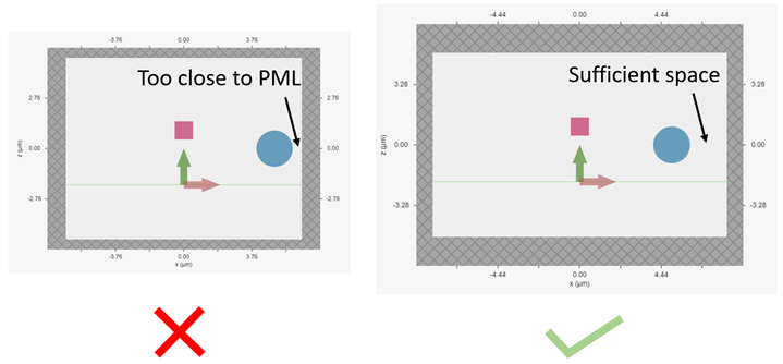
- Move PML boundaries further away from structure interfaces inside the simulation domain, or from sources that may be injecting evanescent waves, like PointDipole, UniformCurrentSource, or CustomFieldSource.
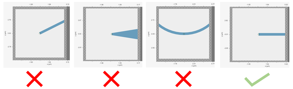
- Make sure structures are translationally invariant into the PML, or if not possible, use Absorber boundaries.
- Remove dispersive materials extending into the PML, or if not possible, use Absorber boundaries.
- If using our fitter to fit your own material data, ensure you are using the
plugins.StableDispersionFitter. - If none of the above work, try using StablePML or Absorber boundaries anyway (note: these may introduce more reflections than in usual simulations with regular PML).
How can I troubleshoot a diverged FDTD simulation?
Structures Inserted into PML at an Angle
Dispersive Material into PML
Evanescent Field Leaks into PML
Gain Medium from Fitting
Courant Factor is Too Large
Additional Notes on Absorber
Contact Tidy3D Support
Why did my simulation finish early?
By default, Tidy3D periodically checks the total field intensity left in the simulation, and compares that to the maximum total field intensity recorded at previous times. If it is found that the ratio of these two values is smaller than \(10^{-5}\), the simulation is terminated as the fields remaining in the simulation are deemed negligible. The shutoff value can be controlled using the Simulation.shutoff parameter or completely turned off by setting it to zero. In most cases, the default behavior ensures that results are correct while avoiding unnecessarily long run times. The Flex Unit cost of the simulation is also proportionally scaled down when early termination is encountered.
Should I make sure that fields have fully decayed by the end of the simulation?
When early termination happens, you may sometimes get a warning that the fields remaining in the simulation at the end of the run have not decayed down to the pre-defined shutoff value. This should usually be avoided (that is to say, Simulation.run_time should be increased), but there are some cases in which it may be inevitable. The important thing to understand is that in such simulations, frequency-domain results cannot always be trusted. The frequency-domain response obtained in the FDTD simulation only accurately represents the continuous-wave response of the system if the fields at the beginning and at the end of the time stepping are (very
close to) zero. That said, there could be non-negligible fields in the simulation. Yet, the data recorded in a given monitor can still be accurate if the leftover fields are no longer passing through the monitor volume. From the point of view of that monitor, fields have already fully decayed. However, there is no way to automatically check this. The accuracy of frequency-domain monitors when fields have not fully decayed is also discussed in one of our FDTD 101
videos.
The primary use case in which you may want to ignore this warning is when you have high-Q modes in your simulation that would require an extremely long run time to decay. In that case, you can use the ResonanceFinder plugin to analyze the modes, as well as field monitors with apodization to capture the modal profiles. The only thing to note is that the normalization of these modal profiles would be arbitrary and would depend on the exact run time and apodization definition. An example of such a use case is presented in our high-Q photonic crystal cavity case study.
Can I have structures larger than the simulation domain?
Structures can indeed be larger than the simulation domain in Tidy3D. In such cases, Tidy3D will automatically truncate the geometry that goes beyond the domain boundaries. For best results, structures that intersect with absorbing boundaries or simulation edges should extend all the way through. In many such cases, an “infinite” size td.inf can be used to define the size along that dimension.
Why can I not change Tidy3D instances after they are created?
You may notice in Tidy3D versions 1.5 and above that it is no longer possible to modify instances of Tidy3D components after they are created. Making Tidy3D components immutable like this was an intentional design decision intended to make Tidy3D safer and more performant.
For example, Tidy3D contains several "validators" on input data. If models are mutated, we can't always guarantee that the resulting instance will still satisfy our validations, and the simulation may be invalid.
Furthermore, making the objects immutable allows us to cache the results of many expensive operations. For example, we can now compute and store the simulation grid without worrying about the value becoming stale later, which significantly speeds up plotting and other operations.
If you have a Tidy3D component that you want to recreate with a new set of parameters, instead of obj.param1 = param1_new, you can call obj_new = obj.copy(update=dict(param1=param1_new)). Note that you may also pass more key value pairs to the dictionary in update. Also, note you can use a convenience method obj_new = obj.updated_copy(param1=param1_new), which is just a shortcut to the obj.copy() call above.
Why are some materials not showing up?
Tidy3D resolves material overlap by their priority - see here for details.
If the priority matches what is needed and the material overlap still does not appear, be sure to check symmetry settings, as the specified symmetry must match the structure symmetry of the simulation.
Why does the kernel crash sometimes when using the web-based Python notebook?
The web-based Python notebook environment in tidy3d.simulation.cloud only has access to 8 GB of memory. When running a large simulation or complex optimizations, the memory needed to process the data could exceed the limit, causing the kernel to crash. In this case, we recommend installing Tidy3D on your local computer by following the installation guide and video. It will then use your computer memory, which is typically larger than 8 GB.
If symmetries are not used in the simulation, memory usage can be reduced by calling data = sim_data.monitor_data['monitor_name'] instead of data = sim_data['monitor_name']. The latter creates a copy of the monitor data and expands it to include the symmetric parts, if applicable.
However, if symmetries are used in the simulation, data = sim_data.monitor_data['monitor_name'] will return data only for the simulated portion of the volume, and not the symmetric extensions. For example, if symmetry is applied in the x-plane, only half of the data will be returned.
Note that many analyses can still be performed with this partial data. For instance, the mode volume can be computed using the non-expanded monitor and then multiplied by the appropriate factor (2, 4, or 8 for 1, 2, or 3 symmetry planes, respectively). An example of this approach can be seen in this example.
How to debug SSL communication issues?
How to debug SSL communication issues?
Users operating within corporate networks, through a VPN, or behind a proxy server may sometimes encounter SSL errors when running the tidy3d python client in their local machines. Note you can always use the python client with our cloud-hosted notebook server.
These errors can occur because the corporate network’s security measures, intercepts, and re-encrypts HTTPS traffic.
A common error message looks like this:
requests.exceptions.SSLError: HTTPSConnectionPool(host='tidy3d-api.simulation.cloud', port=443): Max retries exceeded with url: ... (Caused by SSLError(SSLCertVerificationError(1, '[SSL: CERTIFICATE_VERIFY_FAILED] certificate verify failed: unable to get local issuer certificate ...')))
Note that sometimes, SSL errors can also manifest as authentication errors, or communication timeout errors.
In this FAQ, we will overview some steps to help you debug and resolve this issue.
Step 0: Windows quick fix
Sometimes on Windows running the following will resolve the problem right away. Try this first:
pip install pip-system-certs
If this doesn’t work, proceed with the rest of this guide.
Step 1: The Recommended & Most Secure Solution
The most robust and secure solution is to have your IT department add the Tidy3D SSL certificate to your system’s trust store. This allows your machine to verify our servers’ identity correctly without disabling security features.
Action: Please ask your network administrator to whitelist the API endpoint https://tidy3d-api.simulation.cloud and install the following root certificate https://github.com/flexcompute/tidy3d/blob/develop/tidy3d/web/api/cacert.pem
If these steps do not resolve your issue, please contact our support team and provide the logs from the commands you have tried.
Step 2: Verify Your Environment and Connectivity
Before changing any settings, let’s make sure you can reach the Tidy3D servers.
Test connectivity using ping. This helps confirm if the issue is with SSL verification or basic network access. You should run these commands from your command line (Terminal, PowerShell, or the Anaconda Prompt).
-
Test connection to the web server:
○ → ping -c 3 tidy3d.simulation.cloud PING tidy3d.simulation.cloud (3.160.231.60) 56(84) bytes of data. 64 bytes from server-3-160-231-60.mad53.r.cloudfront.net (3.160.231.60): icmp_seq=1 ttl=245 time=58.7 ms 64 bytes from server-3-160-231-60.mad53.r.cloudfront.net (3.160.231.60): icmp_seq=2 ttl=245 time=77.9 ms 64 bytes from server-3-160-231-60.mad53.r.cloudfront.net (3.160.231.60): icmp_seq=3 ttl=245 time=69.2 ms --- tidy3d.simulation.cloud ping statistics --- 3 packets transmitted, 3 received, 0% packet loss, time 2002ms rtt min/avg/max/mdev = 58.661/68.594/77.930/7.877 ms -
Test connection to the API endpoints:
○ → curl -X GET https://tidy3d-api.simulation.cloud
{
  "error" : "Unauthorized",
  "detail" : "Access is denied",
  "code" : "401",
  "httpStatus" : "401 UNAUTHORIZED",
  "warning" : ""
}
Expected output: A
401 Unauthorizederror message. This is good news; it means you can reach our API server, and the problem is likely with authentication or SSL certificate verification.
Note that many networks can block ping messages so this is not a foolproof check.
Step 3: Disable SSL Verification (Quick Workaround)
As a temporary solution, you can instruct tidy3d to bypass SSL certificate verification. This is not ideal for security but is useful for confirming the source of the problem.
This is done by setting the TIDY3D_SSL_VERIFY environment variable to false.
Setting the Environment Variable:
-
On Windows (in Command Prompt):
set TIDY3D_SSL_VERIFY=falseTo set it permanently, use
setx TIDY3D_SSL_VERIFY false. -
On macOS or Linux (in a bash terminal):
export TIDY3D_SSL_VERIFY="false"
Note thet the user could run into unexpected server communication issues by disabling SSL. This is not recommended.
Verifying the Environment Variable:
It is essential to ensure the variable is set correctly within the environment where you run your script.
-
In your terminal, run the following command.
- Windows:
echo %TIDY3D_SSL_VERIFY% - macOS/Linux:
echo $TIDY3D_SSL_VERIFY - The output should be
false.
- Windows:
-
Inside your Python script, add these lines to the top to see what value the script is reading:
import os
print(f"TIDY3D_SSL_VERIFY is set to: {os.getenv('TIDY3D_SSL_VERIFY')}")
When you run your script, you should see the confirmation printed. If you see None or an empty string, the variable was not set correctly in your current session.
Step 4: Run a Diagnostic Script
If the issue persists, running a minimal script can help isolate the problem to the requests library, which tidy3d uses for communication.
- Save the following code as a Python file (e.g.,
test_connection.py). - Set the
TIDY3D_API_KEYandTIDY3D_SSL_VERIFYenvironment variables in your terminal as shown in Step 2. - Run the script with
python test_connection.py.
# test_connection.py
import os
import requests
from tidy3d.web.core.constants import HEADER_APIKEY
from tidy3d.web.core.environment import Env

def auth(req):
    """Adds the API key to the request header."""
    # Ensure TIDY3D_API_KEY is set in your environment
    req.headers[HEADER_APIKEY] = os.getenv("TIDY3D_API_KEY")
    return req

# Let tidy3d's environment configuration read the SSL variable
# It reads from the TIDY3D_SSL_VERIFY environment variable.
ssl_verify_setting = Env.current.ssl_verify

print(f"API Endpoint: {Env.current.web_api_endpoint}")
print(f"SSL Verification Enabled: {ssl_verify_setting}")

if not ssl_verify_setting:
    # Suppress the warning that will be printed for unverified requests
    requests.packages.urllib3.disable_warnings(requests.packages.urllib3.exceptions.InsecureRequestWarning)
    print("InsecureRequestWarning suppressed.")

try:
    req = requests.Request("GET", f"{Env.current.web_api_endpoint}/apikey")
    auth(req)
    resp = requests.get(req.url, headers=req.headers, verify=ssl_verify_setting)

    print(f"Response: {resp}")
    print(f"Status Code: {resp.status_code}")
    print(f"Response Content: {resp.content}")

except requests.exceptions.SSLError as e:
    print(f"\nCaught an SSLError. This is the core issue.\nDetails: {e}")

except Exception as e:
    print(f"\nAn unexpected error occurred: {e}")
With TIDY3D_SSL_VERIFY set to false and TIDY3D_API_KEY set correctly, the expected output is a status code: 200 and content containing your API key. You will also see an InsecureRequestWarning if you don’t suppress it.
Mediums
How do I include material dispersion?
Dispersive materials are supported in Tidy3D, and we provide an extensive material library with pre-defined materials. Standard dispersive material models can also be defined. If you need help inputting a custom material, let us know!
It is important to keep in mind that dispersive materials are inevitably slower to simulate than their dispersion-less counterparts, with complexity increasing with the number of poles included in the dispersion model. For simulations with a narrow range of frequencies of interest, it may sometimes be faster to define the material through its real and imaginary refractive index at the center frequency. This can be done by defining directly a value for the real part of the relative permittivity $\mathrm{Re}(\epsilon_r)$ and electric conductivity $\sigma$ of a Medium, or through a real part $n$ and imaginary part $k$. The relationship between the two equivalent models is $\mathrm{Re}(\epsilon_r) = n^2 - k^2$, $\mathrm{Im}(\epsilon_r) = 2nk$, and $\sigma = 2 \pi f \epsilon_0 \mathrm{Im}(\epsilon_r)$.
In the case of (almost) lossless dielectrics, the dispersion could be negligible in a broad frequency window, but generally, it is importat to keep in mind that such a material definition is best suited for single-frequency results.
For lossless, weakly dispersive materials, the best way to incorporate the dispersion without doing complicated fits and without slowing the simulation down significantly is to provide the value of the refractive index dispersion $\mathrm{d}n/\mathrm{d}\lambda$ in Sellmeier.from_dispersion(). The value is assumed to be at the central frequency or wavelength (whichever is provided), and a one-pole model for the material is generated. These values are, for example, readily available from the refractive index database.
Can I import my own tabulated material data?
Yes, users can import their own tabulated material data and fit it using one of Tidy3D’s dispersion fitting tools. The FastDispersionFitter tool performs an optimization to find a medium defined as a dispersive PoleResidue model that minimizes the RMS error between the model results and the data. The user can provide data through one of the following methods:
- Numpy arrays directly by specifying
wvl_um,n_data, and optionallyk_data. - A data file with the
from_fileutility function. The data file has columns for wavelength ($μm$), the real part of the refractive index ($n$), and the imaginary part of the refractive index ($k$). $k$ data is optional. Note:from_fileusesnp.loadtxtunder the hood, so additional keyword arguments for parsing the file follow the same format asnp.loadtxt. - URL link to a CSV/TXT file that contains wavelength ($μm$), $n$, and optionally $k$ data with the
from_urlutility function. URL can come from refractiveindex.
This notebook provides detailed instructions and examples of using the fitter.
How do I create a lossy material (with a conductivity)?
To create a lossy material including conductivity, use the tidy3d.Medium object and set the conductivity parameter. For example:
lossy_medium = tidy3d.Medium(permittivity=2.0, conductivity=1.0)How do I create a material from n, k values at a given frequency?
To create a material from the real ($n$) and imaginary ($k$) parts of refractive index, use the tidy3d.Medium.from_nk(). For example:
nk_medium = tidy3d.Medium.from_nk(n=2.0, k=1.0, freq=freq0)Negative $k$ value corresponds to a gain medium. It is only allowed when the parameter
allow_gainis set toTrue.
How do I create a material from optical n, k data?
You can import your own tabulated material data and fit it using one of Tidy3D’s dispersion fitting tools. The FastDispersionFitter tool performs an optimization to find a medium defined as a dispersive PoleResidue model that minimizes the RMS error between the model results and the data. The user can provide data through one of the following methods:
- Numpy arrays directly by specifying
wvl_um,n_data, and optionallyk_data. - A data file with the
from_fileutility function. The data file has columns for wavelength ($μm$), the real part of the refractive index ($n$), and the imaginary part of the refractive index ($k$). $k$ data is optional. Note:from_fileusesnp.loadtxtunder the hood, so additional keyword arguments for parsing the file follow the same format asnp.loadtxt. - URL link to a CSV/TXT file that contains wavelength ($μm$), $n$, and optionally $k$ data with the
from_urlutility function. URL can come from refractiveindex.
This notebook provides detailed instructions and examples on using the fitter.
How do I create a dispersive material from model parameters?
To create a dispersive material from model parameters, you only need to instantiate the medium object and provide its parameters. For example, debye_medium = td.Debye(eps_inf=2.0, coeffs=[(1,2),(3,4)]).
How do I create an anisotropic material?
To create fully anisotropic mediums including all 9 components of the permittivity and conductivity tensors, you can use the tidy3d.FullyAnisotropicMedium object. The provided permittivity tensor and the symmetric part of the conductivity tensor must have coinciding main directions. However, a non-symmetric conductivity tensor can be used to model magneto-optic effects. Note that dispersive properties and subpixel averaging are currently not supported for fully anisotropic materials.
from tidy3d import FullyAnisotropicMedium

perm = [[2, 0, 0], [0, 1, 0], [0, 0, 3]]
cond = [[0.1, 0, 0], [0, 0, 0], [0, 0, 0]]
anisotropic_dielectric = FullyAnisotropicMedium(permittivity=perm, conductivity=cond)Alternatively, you can create a diagonally anisotropic material, using the tidy3d.AnisotropicMedium(xx=medium_xx, yy=medium_yy, zz=medium_zz) object, and then include three medium objects defining the diagonal elements of the permittivity tensor. In this case, the medium objects can be of type Medium, PoleResidue, Sellmeier, Lorentz, Debye, or Drude. Because these diagonal entries are standard medium models, they follow the usual material preprocessing path, including subpixel averaging where the relevant solver or workflow supports it. For example:
from tidy3d import AnisotropicMedium, Medium

medium_xx = Medium(permittivity=4.0)
medium_yy = Medium(permittivity=4.1)
medium_zz = Medium(permittivity=3.9)
anisotropic_dielectric = AnisotropicMedium(xx=medium_xx, yy=medium_yy, zz=medium_zz)How do I create an active material?
allow_gain=True in any medium, e.g. tidy3d.Medium(permittivity=2.0, conductivity=-1.0, allow_gain=True).How do I create a spatially varying material?
How do I export a spatially varying medium dataset to HDF5?
To export a spatially varying medium dataset to a HDF5 file you should use the to_hdf5(filename) method. In the example below, we illustrate how to do that after creating a tidy3d.CustomMedium.
# The coordinate for the refractive index data that includes x, y, z, and frequency
X = np.linspace(-20, 20, 100)  # x grid
Y = np.linspace(-20, 20, 100)  # y grid
Z = [0]  # z grid

# Create a permittivity dataset and a custom medium.
n_data = np.ones((100, 100, 1, 1)) * 12
n_dataset = tidy3d.SpatialDataArray(n_data, coords=dict(x=X, y=Y, z=Z, f=[freq0]))
data = tidy3d.PermittivityDataset(eps_xx=n_dataset, eps_yy=n_dataset, eps_zz=n_dataset)
mat_custom = tidy3d.CustomMedium(eps_dataset=data, interp_method="nearest")

# Export the custom medium dataset to HDF5.
mat_custom.to_hdf5(fname="CustomMedium.hdf5")How do I load a commonly used dispersive material?
from tidy3d import material_library

silver = material_library['Ag']['Rakic1998BB']The key of the dictionary is the abbreviated material name. Some materials have multiple variant models, in which case the second key is the “variant” name.
How can I define a 2D material?
You can create a 2D material using the tidy3d.Medium2D object. This is especially helpful for building very thin materials, like metal layers.
import tidy3d as td

t_copper = 0.0001  # Thickness of the copper layer.
sigma_copper = 50  # Copper conductivity in S/um.

# Define copper as a Medium2D.
copper = td.Medium2D.from_medium(
    td.Medium(conductivity=sigma_copper), thickness=t_copper
)How can I define graphene?
You can create a graphene medium using tidy3d.Graphene, which defines a parametric surface conductivity model for graphene. For example:
import tidy3d as td

gamma = 0.0033  # Scattering rate (eV).
mu_c = 0.5  # Graphene chemical potential (eV).
temp = 300  # Temperature (K).
scaling = 2  # Number of graphene layers.

graphene = td.material_library["graphene"](
    gamma=gamma, mu_c=mu_c, temp=temp, scaling=scaling
).medium

# or
# graphene = td.Graphene(
#    gamma=gamma, mu_c=mu_c, temp=temp, scaling=scaling
# ).mediumHow can I define a nonlinear material?
To create a nonlinear material, define one or more nonlinear models, collect them in a tidy3d.NonlinearSpec, and pass that specification to the nonlinear_spec parameter of the medium. For example:
import tidy3d

nonlinear_model = tidy3d.NonlinearSusceptibility(chi3=1)
nonlinear_spec = tidy3d.NonlinearSpec(models=[nonlinear_model], num_iters=5)
medium = tidy3d.Medium(permittivity=2, nonlinear_spec=nonlinear_spec)chi3 is the nonlinear susceptibility and num_iters is the number of iterations used to solve the nonlinear constitutive relation.How Can I Save and Load a Fitted Medium?
After fitting a medium, as described here, it is possible to save the fitted medium as an hdf5 file and save time when using it in another model. To save the file, just use the .to_file method:
fitted_medium.to_file('medium_name.hdf5')Now, the saved medium can be loaded with the PoleResidue .from_file method:
loaded_medium = td.PoleResidue.from_file('medium_name.hdf5')To use this medium via the web GUI, you have two options:
(a): open the “Material Utilities”, select the “Private Library”, and click the “Upload Material” button;
(b): in the workbench, create a new medium and choose the “Import Material” option in the “Add Medium” panel.
Why Did Results Change for Some Metals in the Material Library?
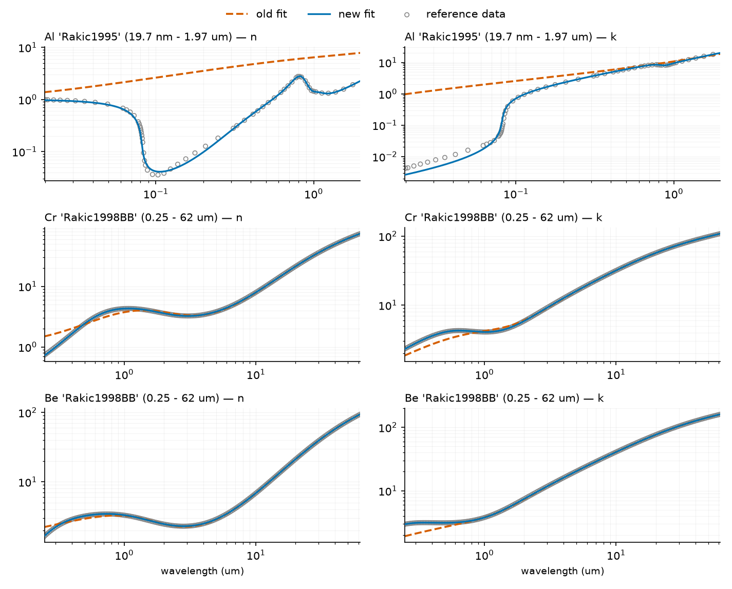
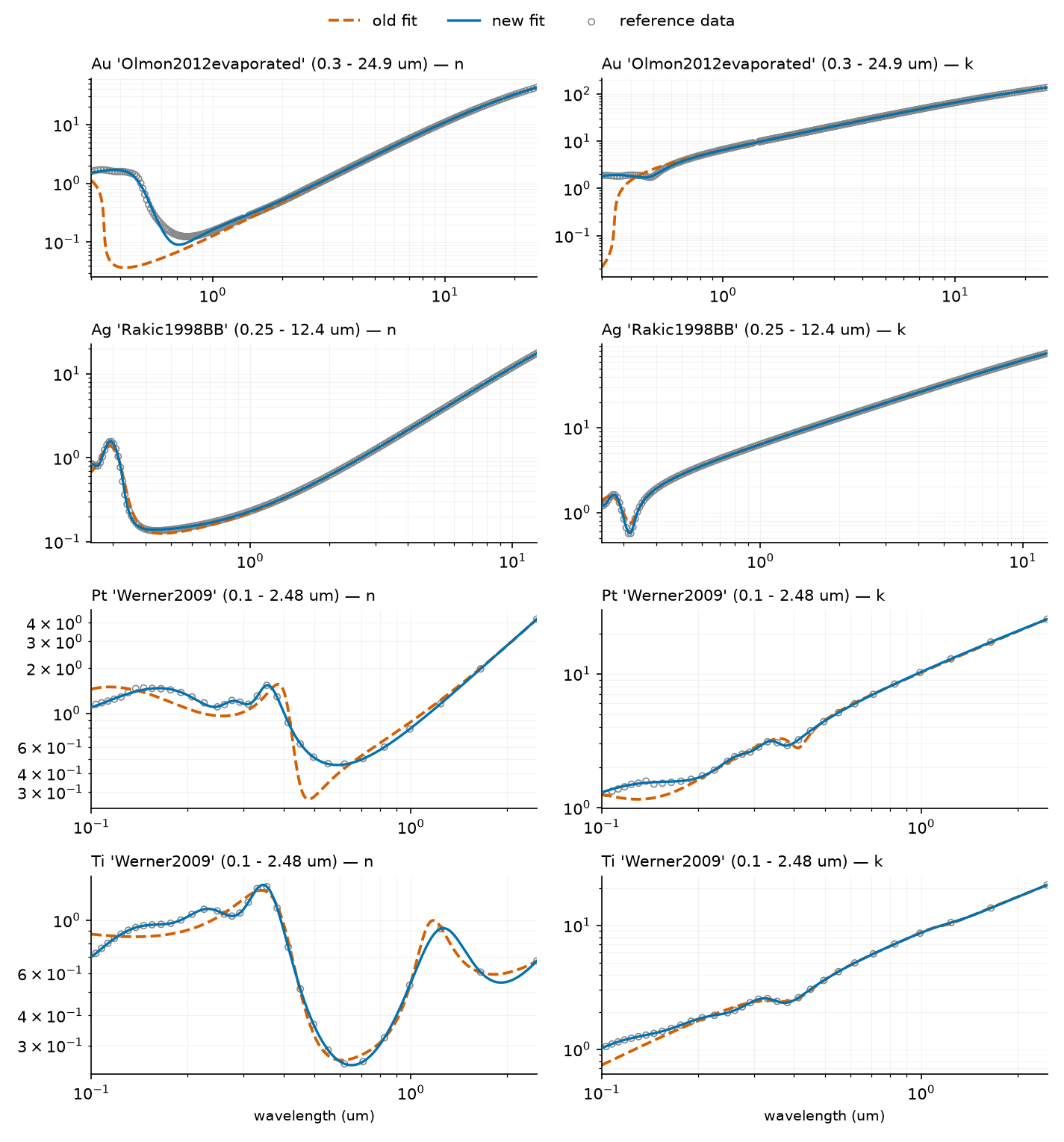
Starting with tidy3d 2.12, the pole-residue fits behind seven metal variants of the material library were replaced, because the previous coefficients did not match their own reference datasets: Al 'Rakic1995', Cr 'Rakic1998BB', Be 'Rakic1998BB', Au 'Olmon2012evaporated', Ag 'Rakic1998BB', Pt 'Werner2009', and Ti 'Werner2009'. Each of these is also the default variant for its material, so simulation results change wherever these materials are used — whether the variant is selected explicitly or via the default — across their entire (unchanged) validity ranges. The worst cases were large: aluminum returned a non-physical real index (n’ of 5–7.5 across the visible and near-IR, where it should be roughly 0.8–1.8), and default gold had no interband response (n = 0.04 at 400 nm where its dataset gives 1.59).
Old vs. new values
Refractive index (n, k) at representative wavelengths — reference data vs. the old and new fits:
| material (variant) | wavelength | data | old fit | new fit |
|---|---|---|---|---|
| Al (‘Rakic1995’) | 100 nm | 0.04, 0.70 | 2.62, 2.58 | 0.04, 0.71 |
| Al | 500 nm | 0.81, 6.05 | 5.12, 6.64 | 0.82, 6.03 |
| Al | 1550 nm | 1.58, 15.66 | 7.29, 15.26 | 1.59, 15.66 |
| Cr (‘Rakic1998BB’) | 637 nm | 3.35, 4.27 | 2.86, 3.57 | 3.35, 4.27 |
| Cr | 10 µm | 7.95, 31.77 | 7.91, 31.78 | 7.95, 31.77 |
| Be (‘Rakic1998BB’) | 300 nm | 2.20, 3.12 | 2.42, 2.12 | 2.21, 3.12 |
| Be | 10 µm | 6.88, 40.81 | 6.88, 40.80 | 6.88, 40.80 |
| Au (‘Olmon2012evaporated’) | 400 nm | 1.59, 1.92 | 0.04, 1.46 | 1.67, 1.84 |
| Au | 5 µm | 3.00, 34.31 | 2.99, 34.31 | 3.00, 34.32 |
| Ag (‘Rakic1998BB’) | 314 nm | 1.03, 0.57 | 1.00, 0.77 | 1.04, 0.58 |
| Ag | 800 nm | 0.19, 4.99 | 0.18, 4.99 | 0.19, 4.99 |
| Pt (‘Werner2009’) | 451 nm | 0.63, 3.76 | 0.33, 3.57 | 0.63, 3.76 |
| Ti (‘Werner2009’) | 500 nm | 0.36, 3.64 | 0.33, 3.63 | 0.36, 3.64 |
The pattern: the old fits were fine in the infrared but wrong in the ultraviolet/visible. The new fits track the reference data at every tabulated point over each variant’s full validity range, and all fits (old and new) are passive and stable.
Full-range comparison (data = circles, old fit = dashed, new fit = solid):
Why the old fits were wrong
The aluminum, chromium, and beryllium coefficients regressed in a 2023 bulk re-fit of the library: fitting each dataset’s full tabulated range with globally weighted least squares lets the infrared tail of a metal’s permittivity (which is thousands of times larger than its visible value) dominate the objective, so the visible-band fit collapses while remaining perfectly passive — no physicality check could catch it. The gold, silver, platinum, and titanium fits were older, low-order fits that under-resolved the visible/interband structure of their datasets. The replacements were fit with an improved vector-fitting backend and are verified against the reference data at every tabulated point, with library-wide accuracy regression tests added so this cannot recur silently.
Am I seeing old or new values? (quick check)
Evaluate the material at a probe wavelength and compare with the table above. The sharpest signatures:
- Al: n’ greater than ~3 anywhere in 500–1700 nm means old (broken) coefficients; new gives n’ = 0.82 / 1.59 at 500 / 1550 nm.
- Au (default): n = 0.04 at 400 nm means old; new gives 1.67.
- Pt: n = 0.33 at 451 nm means old; new gives 0.63.
- Cr: n = 2.86 at 637 nm means old; new gives 3.35.
Simulating only in the infrared? Use the _IR variants
The corrected fits need more poles (up to twice as many), and FDTD cost grows with pole count. Where the previous coefficients matched the reference data to within 2% at every tabulated point over a contiguous infrared band, they remain in the library as lower-cost _IR variants, with validity ranges narrowed to exactly those bands:
| variant | poles (vs. new default) | valid band |
|---|---|---|
td.material_library['Au']['Olmon2012evaporated_IR'] |
3 (vs. 5) | 3.5 – 24.93 µm |
td.material_library['Ag']['Rakic1998BB_IR'] |
3 (vs. 6) | 1.4 – 12.4 µm |
td.material_library['Cr']['Rakic1998BB_IR'] |
3 (vs. 6) | 3.2 – 62 µm |
td.material_library['Be']['Rakic1998BB_IR'] |
4 (vs. 8) | 1.0 – 62 µm |
Inside these bands the _IR variants are as accurate as the new defaults and match pre-update results, so they double as a reproducibility path for infrared studies. There is no _IR variant for Al (the old fit was inaccurate at all wavelengths, infrared included), nor for Pt/Ti (their dataset ends at 2.48 µm, so there is no infrared band to certify). Using a variant outside its valid band produces the standard validity-range warning.
Reproducing results computed with the old coefficients
The recommended way to keep a study self-consistent is to pin the tidy3d version it started with. For infrared-band studies of Au, Ag, Cr, or Be, the _IR variants above are the old coefficients. Otherwise, the old coefficients can be used directly as custom media (they remain valid PoleResidue models — inaccurate against the reference data, but passive and stable):
import tidy3d as td

# Pre-update ('legacy') coefficients of the re-fit variants. These do NOT match
# the reference data (that is why they were replaced); use them only to
# reproduce results computed before the update.
LEGACY_MEDIUMS = {
    ("Al", "Rakic1995"): td.PoleResidue(
        eps_inf=1.0,
        poles=[
            ((-176076476399307.25-0j), (-2.0497198166085053e+17-0j)),
            ((-55958309702844.36-0j), (-1.9328759376610138e+18-0j)),
            ((-32886941985772.406-0j), (2.985600009810314e+17-0j)),
            ((-836904963.7321033-0j), (1.9664479588602982e+18-0j)),
        ],
        frequency_range=(151926744799612.75, 1.5192674479961274e+16),
    ),
    ("Cr", "Rakic1998BB"): td.PoleResidue(
        eps_inf=1.0,
        poles=[
            ((-73056488139432.73-0j), (-2.7457982793225763e+17-0j)),
            ((-145384800564.84518-0j), (2.8558672134946093e+17-0j)),
            ((-2137728163059224-740097502616341.5j), (5846984237158586+9.545555973191486e+16j)),
        ],
        frequency_range=(4835362227919.29, 1208840556979822.5),
    ),
    ("Be", "Rakic1998BB"): td.PoleResidue(
        eps_inf=1.0,
        poles=[
            ((-1737739552967275.2-0j), (2.3924381023090224e+16-0j)),
            ((-151352273074186.28-0j), (4367049766016236.5-0j)),
            ((-53296876831178.09-0j), (-6.001139611206947e+17-0j)),
            ((-20238020062.550835-0j), (6.055916356024831e+17-0j)),
        ],
        frequency_range=(4835978484543.8545, 1208994621135963.5),
    ),
    ("Au", "Olmon2012evaporated"): td.PoleResidue(
        eps_inf=5.632132676065586,
        poles=[
            ((-208702733035001.06-205285605362650.1j), (-5278287093117479+1877992342820785.5j)),
            ((-5802337384288.284-6750566414892.662j), (4391102400709820+6.164348337888482e+18j)),
            ((-56597670698540.76-8080114483410.944j), (895004078070708.5+5.346045584373232e+18j)),
        ],
        frequency_range=(12025369359446.29, 999308193769986.8),
    ),
    ("Ag", "Rakic1998BB"): td.PoleResidue(
        eps_inf=2.080628548409516,
        poles=[
            ((-74116405167315.4-0j), (-1.0385354711010449e+18-0j)),
            ((-199290207342.26654-0j), (1.0396417727844411e+18-0j)),
            ((-622425347820110.2-6539570627133650j), (936046890626063+1966533189396127.8j)),
        ],
        frequency_range=(24179892422719.273, 1208994621135963.5),
    ),
    ("Pt", "Werner2009"): td.PoleResidue(
        eps_inf=1.0,
        poles=[
            ((-9288886703545810-1.9809701816539028e+16j), (-2559720539992317+2.619854823299511e+16j)),
            ((-113303296165008.06-132666543091888.84j), (5059991338597539+1.459321906232765e+18j)),
            ((-525913270217765.06-4665172268701287j), (4280438237239983.5+1882099733932914.8j)),
        ],
        frequency_range=(120884055879414.03, 2997924585809468.0),
    ),
    ("Ti", "Werner2009"): td.PoleResidue(
        eps_inf=1.0,
        poles=[
            ((-1316659173032264.2-4853426451943540j), (6846803510207887+3451315459947241.5j)),
            ((-234898849175817.28-1643952885872075.5j), (-1039094910406333.4+2786587583155544.5j)),
            ((-9631968003009.37-107553157768951.47j), (5856843593653923+1.1954179403843133e+18j)),
        ],
        frequency_range=(120884055879414.03, 2997924585809468.0),
    ),
}
# example: reproduce pre-2.12 default aluminum
old_al = LEGACY_MEDIUMS[("Al", "Rakic1995")]Structures
How do I import a structure from a GDSII file?
In Tidy3D, complex structures can be imported from GDSII files via the third-party gdstk package, which you can install running pip install gdstk. To load the geometry from a GDSII file, you should select the cell with the geometry you want. It is usually easier to verify that we can find the correct one by name first, for example:
# Load a GDSII library from the file.
lib_loaded = gdstk.read_gds(gds_path)

# Create a cell dictionary with all the cells in the file.
all_cells = {c.name: c for c in lib_loaded.cells}
print("Cell names: " + ", ".join(all_cells.keys()))Then you can construct Tidy3D geometries from the GDS cell just loaded, along with other information such as the axis, sidewall angle, and bounds of the "slab" using tidy3d.Geometry.from_gds(). When loading GDS cell as the cross section of the device, we can tune reference_plane to set the cross-section to lie at bottom, middle, or top of the generated geometry with respect to the axis. E.g. if axis=1, bottom refers to the negative side of the y-axis, and top refers to the positive side of the y-axis. Additionally, we can optionally dilate or erode the cross section by setting dilation. A negative dilation corresponds to erosion. Note, we have to keep track of the gds_layer and gds_dtype used to define the GDS cell earlier, so we can load the right components.
wg_height = 0.22
dilation = 0.02

geo = tidy3d.Geometry.from_gds(
    gds_cell=all_cells["TOP"],
    gds_layer=0,
    gds_dtype=0,
    axis=2,
    slab_bounds=(-0.11, 0.11),
    reference_plane="bottom",
)You can find more details on importing GDSII files in these notebooks: Importing GDS files; Defining self-intersecting polygons.
How can I import a structure from STL files?
To use the STL import functionality, you must install Tidy3D as pip install "tidy3d[trimesh]", which will install optional dependencies for processing surface meshes. Then you can use the tidy3d.TriangleMesh.from_stl() function. In the following example, we will import a simple box geometry from a STL file.
# Make the geometry object representing the STL solid from the STL file stored on disk
box = tidy3d.TriangleMesh.from_stl(
    filename="./misc/box.stl",
    scale=1,  # The units are already microns as desired, but this parameter can be used to change units [default: 1].
    origin=(
        0,
        0,
        0,
    ),  # This can be used to set a custom origin for the stl solid [default: (0, 0, 0)]
    solid_index=None,  # Sometimes, there may be more than one solid in the file; use this to select a specific one by index.
)See this example for a complete reference on importing STL files.
How do I export a structure to GDSII format?
In Tidy3D, you can export structures to GDSII file via the third-party gdstk package, which you can install running pip install gdstk. The example below creates a simple geometry and then exports it to GDSII:
# Create a gds cell to add the structures to.
geo_cell = gdstk.Cell("TOP")

# Make a box and add it to the cell.
box = gdstk.rectangle((-1, 1), (-1, 1), layer=0)
geo_cell.add(box)

# Create a library for the cell and save it.
gds_path = "box.gds"
lib = gdstk.Library()
lib.add(geo_cell)
lib.write_gds(gds_path)The method .to_gds_file() is another option to export a geometry to GDSII. For example:
# Create a simulation object.
sim = td.Simulation(
    size=sim_size,
    grid_spec=td.GridSpec.uniform(dl=dl),
    structures=structures,
    boundary_spec=td.BoundarySpec.all_sides(boundary=td.PML()),
)

# Export the structure to GDSII.
sim.to_gds_file(fname="sim.gds",
  z=0,
  permittivity_threshold=5,
  frequency=f0,
)You can find more details on exporting structures to GDSII files in the notebook Importing GDS files.
How do I create a box?
You can create a box geometry using the tidy3d.Box object. You can specify the center and size parameters, as below:
box = tidy3d.Box(center=(1,2,3), size=(2,2,2))Or you can use the tidy3d.Box.from_bounds() method, where you should define the rmin and rmax coordinates of the lower and upper box corners. For example:
box = tidy3d.Box.from_bounds(
  rmin=(-10, -1, -0.1),
  rmax=(10, 1, 0.1),
)How do I create a sphere?
You can create a sphere using the tidy3d.Sphere object and specifying the center and radius parameters, as below:
sphere = tidy3d.Sphere(
    center=(0, 0, 0),
    radius=1,
)How do I create a cylinder?
You can create a cylinder using the tidy3d.Cylinder object. In the example below we create a cylinder 2 $\mu$m in length, oriented along the z-axis, with a 0.5 $\mu$m radius, and positioned at (-1,1,0). To obtain a conical shape, set the parameters sidewall_angle and reference_plane.
cyl = tidy3d.Cylinder(center=(-1,1,0), radius=0.5, length=2, axis=2)How do I create a polygon?
Use the tidy3d.PolySlab object to create an extruded polygon with an optional sidewall angle along the axis direction. The polygon geometry is defined by the vertices parameter, which receives a list of (d1, d2) coordinates defining the geometry of the polygon face at the reference_plane. The slab_bounds parametere defines the minimum and maximum positions of the slab along the axis dimension. Set the sidewall_angle with respect to the reference_plane to create slanted sidewalls. In addition, you can dilate or erode the polygon by setting positive or negative values to dilation parameter.
vertices = np.array([(0,0), (1,0), (1,1)])
triangle = tidy3d.PolySlab(vertices=vertices, axis=2, slab_bounds=(-1, 1))How do I create a geometry group?
A geometry group is a convenient way to gather multiple geometry objects into one collection. It can significantly improve performance when all the geometries in the group are assigned to the same medium. To create a geometry group, use the tidy3d.GeometryGroup object and set the geometries parameter as below:
cylinders = []

for i in range(0, 4):
  c = tidy3d.Cylinder(
    axis=2, radius=0.3, center=(i, 0, 0), length=2,
  )
  cylinders.append(c)

structure = tidy3d.Structure(
  geometry=tidy3d.GeometryGroup(geometries=cylinders),
  medium=tidy3d.Medium(permittivity=4),
)How do I combine multiple geometries?
You can combine multiple geometries using the tidy3d.ClipOperation object to perform ‘union’, ‘intersection’, ‘difference’, and ‘symmetric_difference’ operations. For example:
box = tidy3d.Box(center=(0,0,0), size=(1, 1, 2))
cyl = tidy3d.Cylinder(center=(1,0,0), radius=0.5, length=2, axis=2)

union = tidy3d.ClipOperation(
  operation='union', geometry_a=box, geometry_b=cyl
)

intersection = tidy3d.ClipOperation(
  operation='intersection', geometry_a=box, geometry_b=cyl
)

difference = tidy3d.ClipOperation(
  operation='difference', geometry_a=box, geometry_b=cyl
)

symmetric_difference = tidy3d.ClipOperation(
  operation='symmetric_difference', geometry_a=box, geometry_b=cyl
)When two structures overlap, what is the priority determined?
When two structures overlap, the last ones in the structures list will override the permittivities of the previous structures. This notebook illustrates how to use this rule to create a photonic crystal slab. The holes geometry with a refractive index of 1 overrides the slab permittivities in regions where they overlap, creating the air holes.
# Simulation
sim = td.Simulation(
    size=sim_size,
    grid_spec=grid_spec,
    structures=[slab, holes],
    sources=[source],
    monitors=[time_series_mnt, field_mnt, far_field_mnt],
    run_time=run_time,
    boundary_spec=td.BoundarySpec.all_sides(boundary=td.PML()),
    symmetry=(1, -1, 1),
    shutoff=0,
)How to rotate a geometry?
In Tidy3D, all geometries can be translated, rotated, and scaled. These methods create a new copy of the original geometry with a transformation applied. For example, you can start with a tidy3d.Box centered at the origin and create a copy of it rotated around the z-axis:
box = tidy3d.Box(size=(2, 1, 1))

rotated_box = box.rotated(np.pi / 6, axis=2)

_ = rotated_box.plot(z = 0)See this example for more information.
How to translate a geometry?
In Tidy3D, all geometries can be translated, rotated, and scaled. These methods create a new copy of the original geometry with a transformation applied. For example, you can start with a tidy3d.Box centered at the origin and create a copy of it translated in the x-direction by 2 $\mu m$:
box = tidy3d.Box(size=(2, 1, 1))

box_translated = box.translated(x=2, y=0, z=0)

_ = box_translated.plot(z = 0)See this example for more information.
How to scale a geometry?
In Tidy3D, all geometries can be translated, rotated, and scaled. These methods create a new copy of the original geometry with a transformation applied. For example, you can start with a tidy3d.Box centered at the origin and create a copy of it scaled by a factor of 2 in all directions:
box = tidy3d.Box(size=(2, 1, 1))

box_scaled = box.scaled(x=2.0, y=2.0, z=2.0)

_ = box_scaled.plot(z = 0)See this example for more information.
How can I apply transformations to a geometry?
In Tidy3D, all geometries can be translated, rotated, and scaled. These methods create a new copy of the original geometry with a transformation applied. For example, you can start with a tidy3d.Box centered at the origin and create a copy of it rotated around the z-axis:
import numpy as np
import tidy3d

box = tidy3d.Box(size=(2, 1, 1))

rotated_box = box.rotated(np.pi / 6, axis=2)

_ = rotated_box.plot(z = 0)Transformed geometries can be further transformed. Composing transformations is as simple as cascading the method calls. In the following example, we create an ellipsoidal prism by scaling a primitive tidy3d.Cylinder and rotating it.
import numpy as np
import tidy3d

ellipsoid = tidy3d.Cylinder(radius=0.5, length=0.5, axis=1).scaled(x=2, y=1, z=1).rotated(np.pi / 4, axis=1)

_ = ellipsoid.plot(y=0)A tidy3d.Transformed object contains an inner geometry and a transformation, written as a 4 x 4 matrix and applied to the (homogeneous) coordinates of the inner geometry. It is possible to define a Transformed object directly from the inner geometry and the transformation. To help create the most usual transformation matrices, the Transformed class has 3 static methods for translation, rotation, and scaling that can be used and combined (the @ operator can be used for matrix multiplication with numpy arrays).
import numpy as np
import tidy3d

rot = tidy3d.Transformed.rotation(np.pi / 3, axis=(1, 1, 1))
trans = tidy3d.Transformed.translation(1, 2, 0)
scale = tidy3d.Transformed.scaling(1, 1.25, 1)

# The box is first rotated, then translated, and finally scaled
transformed = tidy3d.Transformed(
    geometry=tidy3d.Box(size=(1, 1, 1)),
    transform=scale @ trans @ rot,
)See this example for more information.
How do I use clip operations?
You can use the tidy3d.ClipOperation object to combine multiple geometries through ‘union’, ‘intersection’, ‘difference’, and ‘symmetric_difference’ operations. Simply define the geometry_a and the geometry_b and assign them to the clip object. For example:
box = tidy3d.Box(center=(0,0,0), size=(1, 1, 2))
cyl = tidy3d.Cylinder(center=(1,0,0), radius=0.5, length=2, axis=2)

union = tidy3d.ClipOperation(
  operation='union', geometry_a=box, geometry_b=cyl
)

intersection = tidy3d.ClipOperation(
  operation='intersection', geometry_a=box, geometry_b=cyl
)

difference = tidy3d.ClipOperation(
  operation='difference', geometry_a=box, geometry_b=cyl
)

symmetric_difference = tidy3d.ClipOperation(
  operation='symmetric_difference', geometry_a=box, geometry_b=cyl
)Which features can I use to create geometries in Tidy3D?
Tidy3D offers four primitive geometric shapes: Box, Cylinder, Sphere, and PolySlab. An extensive array of intricate geometrical configurations can be defined from these fundamental building blocks by manipulating their properties and hierarchical arrangements. For instance, our tutorials on the Luneburg lens waveguide size converter and the Fresnel lens showcase the creation of curved surfaces through the strategic layering of cylindrical elements.
Beyond the in-built primitives, Tidy3D accommodates external geometrical specifications in either the GDS or STL file formats, allowing users to import custom geometries created in their preferred design tools. Additionally, compatibility with external libraries like gdstk and shapely opens the gateway to even more complex geometric possibilities. Using gdstk to create various waveguide structures has been demonstrated in various examples, such as thepolarization splitter and rotator based on 90-degree bends](https://www.flexcompute.com/tidy3d/examples/notebooks/90BendPolarizationSplitterRotator/). Additionally, you can create complex geometries using the Trimesh library, as demonstrated in this tutorial.
How do I define complex geometries using trimesh?
To define complex geometries using the Trimesh library, you must install Tidy3D as pip install "tidy3d[trimesh]", which will install optional dependencies needed for processing surface meshes. The Trimesh library provides some built-in geometries such as ring (annulus), box, capsule, cone, cylinder, and so on. Let’s create a ring as an example.
n_sections = 100 # How many sections to discretize the mesh.

# Create a ring mesh.
ring_mesh = trimesh.creation.annulus(r_min=9, r_max=10, height=1, sections=n_sections)

# Plot the mesh.
ring_mesh.show()To use this geometry in a Tidy3D simulation, you need to convert the mesh into a tidy3d.TriangleMesh geometry. Use the from_trimesh() method to conviently convert the mesh to a Tidy3D geometry. From there, you can further define the Tidy3D structure and put it into a simulation.
# Define a tidy3d geometry from a mesh.
ring_geo = td.TriangleMesh.from_trimesh(ring_mesh)This example shows how to create many different complex geometries using Trimesh.
How do I build curves, rings, and other photonic integrated components?
The gdstk library offers a convenient and flexible way to construct commonly used photonic integrated circuit (PIC) components, such as straight waveguides, linear tapers, rings, race tracks, s-bends, circular bends, and directional couplers. This notebook contains pre-defined functions used to construct commonly used PIC components. Users can directly copy these pre-defined functions to their script and use them to build their simulations. More importantly, users can learn the workflow from these examples and create their own Tidy3D structures using the same principles.
How do I build photonic crystal structures?
Tidy3D provides four basic geometric shapes, namely, Box, Cylinder, Sphere, and PolySlab. These shapes can be used to create various periodic structures used in photonic crystals and other photonic devices such as square or hexagonal arrays of cylinders, slabs with square or hexagonal arrays of holes, rectangular grating, L and H cavities, wood pile, and FCC/BCC crystals. For this purpose, you can organize these geometries in a tidy3d.GeometryGroup. This notebook contains functions that can be used to build these popular periodic structures with ease. Moreover, users can learn from these examples and create their own periodic structures using the same principles.
Sources
What source bandwidth should I use for my simulation?
Tidy3D’s broadband source feature is designed to produce the most accurate results in the frequency range of (freq0 - 1.5 * fwidth, freq0 + 1.5 * fwidth). Therefore, it is necessary to define the source center frequency freq0 and bandwidth fwidth to properly cover the desired application frequency range. For example, if the user wants to adjust the source bandwidth to cover a wavelength range between wl_min and wl_max, the source bandwidth can be defined as: fwidth = alpha * (C_0/wl_max - C_0/wl_min), where alpha is a constant typically chosen between 1/3 and 1/2 to ensure accurate results.
How do I set the source frequency and bandwidth?
You can set the source frequency and bandwidth through the source_time parameter, which accepts a tidy3d.GaussianPulse object. In the example below, we create a tidy3d.PointDipole source to radiate power at a center wavelength of 1.55 $\mu$m over a bandwidth of 100 nm.
# Simulation wavelength and bandwidth.
wl = 1.55
bw = 0.1
wl_max = wl + bw / 2
wl_min = wl - bw / 2
freq0 = tidy3d.C_0 / wl
fwidth = 0.5 * (tidy3d.C_0 / wl_min - tidy3d.C_0 / wl_max)

# Source bandwidth.
pulse = tidy3d.GaussianPulse(freq0=freq0, fwidth=fwidth)

# Source definition
pt_dipole = tidy3d.PointDipole(
  center=(1,2,3),
  source_time=pulse,
  polarization='Ex',
  interpolate=True,
  name="dipole",
)How can I plot the source spectrum and time-dependence?
The tidy3d.GaussianPulse object has the built-in functions plot_spectrum and plot that allow users to visualize the source spectrum and time-dependence, respectively. For example:
# Simulation wavelength and bandwidth.
wl = 1.55
bw = 0.1
wl_max = wl + bw / 2
wl_min = wl - bw / 2
freq0 = td.C_0 / wl
fwidth = 0.5 * (td.C_0 / wl_min - td.C_0 / wl_max)
run_time = 1e-12

# Source bandwidth.
pulse = td.GaussianPulse(freq0=freq0, fwidth=fwidth)

# Source definition
pt_dipole = td.PointDipole(
  center=(1,2,3),
  source_time=pulse,
  polarization='Ex',
  interpolate=True,
  name="dipole",
)

fig, (ax1, ax2) = plt.subplots(1, 2, figsize=(12, 4), tight_layout=True)

# Plot the source spectrum.
pt_dipole.source_time.plot_spectrum(
    times=np.linspace(0, run_time, 2000), val="abs", ax=ax1,
)

# Plot the source time-dependence.
pt_dipole.source_time.plot(
    times=np.linspace(0, run_time / 3, 2000), val='real', ax=ax2,
)

plt.show()How can I plot the source spectrum?
When defining a source, you must specify a source time profile, typically Gaussian. For example, we can define a plane wave as
plane_wave = td.PlaneWave(
  source_time=td.GaussianPulse(freq0=freq0, fwidth=0.5 * freqw),
  size=(td.inf, td.inf, 0),
  center=(0, 0, 0.3 * lda0),
  direction="-",
  pol_angle=0,
)Here, the source time is a Gaussian pulse with central frequency freq0 and frequency width 0.5 * freqw. To visualize the spectrum it gives, we can use the plot_spectrum method by
plane_wave.source_time.plot_spectrum(
  times=np.linspace(0, sim.run_time, 2000), val="abs"
)
plt.show()Here, we need to specify the sampled time instances. To ensure the source spectrum is plotted correctly, we need to ensure the time sampling is sufficiently fine and the end time is sufficiently long compared to the pulse width.
How are results normalized?
In many cases, Tidy3D simulations can be run, and well-normalized results can be obtained without normalizing/empty runs. This is because care is taken internally to normalize the injected power, as well as the output results, in a meaningful way. To understand this, there are two separate normalizations that happen, outlined below. Both are discussed with respect to frequency-domain results, as those are the most commonly used.
Source spectrum normalization
Every source has a spectrum associated to its particular time dependence that is imprinted on the fields injected in the simulation. Usually, this is somewhat arbitrary, and it is most convenient to take it out of the frequency-domain results. By default, after a run, Tidy3D normalizes all frequency-domain results by the spectrum of the first
source in the list of sources in the simulation. This choice can be modified using the Simulation.normalize_index attribute, or normalization can be turned off by setting that to None. Results can even be renormalized after the simulation run using SimulationData.renormalize(). If multiple sources are used, but they all have the same time dependence, the default normalization is still meaningful. However, if different sources have a different time dependence, then it may not be
possible to obtain well-normalized results without a normalizing run.
This type of normalization is applied directly to the frequency-domain results. The custom pulse amplitude and phase defined in SourceTime.amplitude and SourceTime.phase, respectively, are not normalized out. This gives the user control over a (complex) prefactor that can be applied to scale any source. Additionally, the power injected by each type of source may have some special normalization, as outlined below.
Source power normalization
Source power normalization is applied depending on the source type. In the cases where normalization is applied, the actual injected power may differ slightly from what is described below due to finite grid effects. The normalization should become exact with sufficiently high resolution. That said, in most cases the error is negligible even at default resolution.
The injected power values described below assume that the source spectrum normalization has also been applied.
-
PointDipole: The point dipole source represents an infinitesimal antenna with a fixed current density. The normalization is such that the power injected by the source in a homogeneous material of refractive index $n$ at frequency $\omega = 2\pi f$ is approximately given as follows
- $\frac{\omega^2}{12\pi}\frac{\mu_0 n}{c}$, 3D simulation, electric current
- $\frac{\omega^2}{12\pi}\frac{\epsilon_0 n^3}{c}$, 3D simulation, magnetic current
- $\frac{\omega \mu_0}{16}$, 2D TE simulation, electric current
- $\frac{\omega \mu_0}{8}$, 2D TM simulation, electric current
- $\frac{\omega \epsilon_0 n^2}{8}$, 2D TE simulation, magnetic current
- $\frac{\omega \epsilon_0 n^2}{16}$, 2D TM simulation, magnetic current
There can be a small difference in the true power compared to the analytical values above due to the finite grid. Note that the current source definition used in Tidy3D is different from the definition of an electric dipole composed of two separated, oscillating electric charges, which is also common. The power normalization differs by a factor of $\omega^2$ for electric dipoles, and $\mu_0^2 \omega^2$ for magnetic dipoles.
-
UniformCurrentSource: No extra normalization applied.
-
CustomFieldSource: No extra normalization applied.
-
ModeSource, PlaneWave, GaussianBeam, AstigmaticGaussianBeam: Normalized to inject 1W power at every frequency. If supplied
SourceTime.num_freqsis1, this normalization is only exact at the central frequency of the associated SourceTime pulse but should still be very close to 1W at nearby frequencies too. Increasingnum_freqscan be used to make sure the normalization works well for a broadband source. The correct usage for a PlaneWave source is to span the whole simulation domain for a simulation with periodic (or Bloch) boundaries, in which case the normalization of this technically infinite source is equivalent to 1W per unit cell. For the other sources which have a finite extent, the normalization is correct provided that the source profile decays by the boundaries of the source plane. Verifying that this is the case is always advised, as otherwise results may be spurious beyond just the normalization (numerical artifacts will be present at the source boundary). -
TFSFSource: Normalized to inject $1W/μm^{2}$ in the direction of the source injection axis. This is convenient for computing scattering and absorption cross-sections without the need for additional normalization. Note that for angled incidence, a factor of $1/\cos(\theta)$ needs to be applied to convert to the power carried by the plane wave in the propagation direction, which is at an angle $\theta$ with respect to the injection axis. Note also that when the source spans the entire simulation domain with periodic or Bloch boundaries, the conversion between the normalization of aTFSFSourceand a PlaneWave is just the area of the simulation domain in the plane normal to the injection axis.
How do I set a PointDipole source?
The tidy3d.PointDipole is a zero-dimensional uniform current source. The example below illustrates how to define tidy3d.PointDipole within a simulation.
# Source bandwidth.
pulse = tidy3d.GaussianPulse(freq0=200e12, fwidth=20e12)

# Source definition
pt_dipole = tidy3d.PointDipole(
  center=(1,2,3),
  source_time=pulse,
  polarization='Ex',
  interpolate=True,
  name="dipole",
)Use the center parameter to set the dipole position, then adjust the source_time dependence using tidy3d.GaussianPulse. The source polarization defines the direction and type of the current component. Finally, the parameter interpolate handles reverse interpolation of zero-size dimensions of the source. If False, the source data is snapped to the nearest Yee grid point. If True, equivalent source data is applied on the surrounding Yee grid points to emulate placement at the specified location using linear interpolation.
See this notebook to an example on setting up a tidy3d.PointDipole source.
How do I calculate the power radiated by a PointDipole source?
The tidy3d.PointDipole source placed in a lossless homogeneous material injects power close to the analytically expected result for an infinitesimal antenna with oscillating current. There can be a small difference from the analytical result due to the finite grid, which disappears in the limit of high resolution. To calculate the radiated power of a dipole in the presence of dispersive, lossy, or non-homogeneous materials, you can use a tidy3d.FluxMonitor box. Refer to this notebook for an example.
How do I set a UniformCurrentSource source?
The tidy3d.UniformCurrentSource is a rectangular volume source with uniform time dependence. The example below illustrates how to define a tidy3d.UniformCurrentSource within a simulation.
# Source bandwidth.
pulse = tidy3d.GaussianPulse(freq0=200e12, fwidth=20e12)

# Source definition
source = tidy3d.UniformCurrentSource(
  center=(1,2,3),
  size=(0,2,1),
  source_time=pulse,
  polarization='Ex',
  interpolate=True,
  name="uniform_source",
)Use the center and size parameters to set the source position and volume, then adjust the source_time dependence using tidy3d.GaussianPulse. The source polarization defines the direction and type of the current component. Finally, the parameter interpolate handles reverse interpolation of zero-size dimensions of the source. If False, the source data is snapped to the nearest Yee grid point. If True, equivalent source data is applied on the surrounding Yee grid points to emulate placement at the specified location using linear interpolation. Note that making size=(0, 0, 0) is equivalent to including a tidy3d.PointDipole source.
How do I set a PlaneWave source?
The tidy3d.PlaneWave is a uniform current distribution on an infinite extent plane. The example below illustrates how to define a tidy3d.PlaneWave within a simulation.
# Source bandwidth.
pulse = tidy3d.GaussianPulse(freq0=200e12, fwidth=20e12)

# Source definition
source = tidy3d.PlaneWave(
  center=(0, 0, 5),
  size=(tidy3d.inf, tidy3d.inf, 0),
  source_time=pulse,
  direction='-',
  pol_angle=np.pi/2,
  angle_theta=0,
  angle_phi=0,
  name="plane_wave",
)Use the center and size parameters to set the source position and dimension, then adjust the source_time dependence using tidy3d.GaussianPulse. The direction parameter specifies propagation in the positive or negative direction of the injection axis. You can change the light polarization using pol_angle, and adjust the propagation axis direction with angle_theta and angle_phito control the polar and azimuth angles.
This example illustrates setting up a tidy3d.PlaneWave source at normal and off-normal incidences.
For oblique incidence, there are two possible settings: fixed in-plane k-vector and fixed-angle mode. The first requires Bloch periodic boundary conditions, and the incidence angle is exact only at the central wavelength. The latter requires periodic boundary conditions and maintains a constant propagation angle over a broadband spectrum. For more information and important notes, refer to this example: Broadband PlaneWave With Constant Oblique Incident Angle.
How Do I Set a Modesource?
The tidy3d.ModeSource injects a current source in the simulation to excite a modal profile in a finite extent plane. It is commonly used to excite specific waveguide modes in photonic integrated circuits. The example below asks for two modes in a silicon-on-insulator (SOI) waveguide operating at 1.55 $\mu$m, groups TE-like modes first, and injects the second returned mode.
# Source bandwidth.
pulse = tidy3d.GaussianPulse(freq0=1.934e14, fwidth=6.245e12)

# Mode specification. Group TE-like modes first, then verify the returned modes.
mode_spec = tidy3d.ModeSpec(
    target_neff=3.47,
    num_modes=2,
    sort_spec=tidy3d.ModeSortSpec(
        filter_key="TE_fraction",
        filter_reference=0.5,
    ),
)

# Source definition.
source = tidy3d.ModeSource(
    center=(0, 0, -2),
    size=(0, 2, 1.5),
    source_time=pulse,
    direction="+",
    mode_spec=mode_spec,
    mode_index=1,  # Select the second returned mode (zero-based).
    name="mode_source",
)You should use the center and size parameters to define a source plane surrounding the waveguide, then adjust the source_time dependence using tidy3d.GaussianPulse. The direction="+" parameter specifies propagation in the positive waveguide axis. The tidy3d.ModeSpec object includes all the specifications of a mode solver, which calculates the optical modes given the material distribution within the source plane. The modes calculated by the mode solver are sorted by decreasing effective index by default. Here, sort_spec uses tidy3d.ModeSortSpec to place TE-like modes first by filtering on TE_fraction >= 0.5; within each group, modes use the default ordering by decreasing effective index. The zero-based mode_index=1 selects the second returned mode, but TE-like grouping does not by itself identify that mode as TE1. Solve and inspect the modal fields and polarization fractions for your specific geometry before choosing the index.
This example illustrates setting up a tidy3d.ModeSource source.
How Do I Inject a Specific Optical Mode in a Waveguide?
To inject a specific optical mode in the waveguide, you can use the tidy3d.ModeSource source. The example below asks for two modes in a silicon-on-insulator (SOI) waveguide operating at 1.55 $\mu$m, groups TE-like modes first, and injects the second returned mode:
# Source bandwidth.
pulse = tidy3d.GaussianPulse(freq0=1.934e14, fwidth=6.245e12)

# Mode specification. Group TE-like modes first, then verify the returned modes.
mode_spec = tidy3d.ModeSpec(
    target_neff=3.47,
    num_modes=2,
    sort_spec=tidy3d.ModeSortSpec(
        filter_key="TE_fraction",
        filter_reference=0.5,
    ),
)

# Source definition.
source = tidy3d.ModeSource(
    center=(0, 0, -2),
    size=(0, 2, 1.5),
    source_time=pulse,
    direction="+",
    mode_spec=mode_spec,
    mode_index=1,  # Select the second returned mode (zero-based).
    name="mode_source",
)You should use the center and size parameters to define a source plane surrounding the waveguide, then adjust the source_time dependence using tidy3d.GaussianPulse. The direction="+" parameter specifies propagation in the positive waveguide axis. The tidy3d.ModeSpec object includes all the specifications of a mode solver, which calculates the optical modes given the material distribution within the source plane. The modes calculated by the mode solver are sorted by decreasing effective index by default. Here, sort_spec uses tidy3d.ModeSortSpec to place TE-like modes first by filtering on TE_fraction >= 0.5; within each group, modes use the default ordering by decreasing effective index. The zero-based mode_index=1 selects the second returned mode, but TE-like grouping does not by itself identify that mode as TE1. Solve and inspect the modal fields and polarization fractions for your specific geometry before choosing the index.
This example illustrates setting up a tidy3d.ModeSource source.
How do I inject an optical mode in a waveguide bend?
To inject an optical mode in a waveguide bend, you must set the bend_radius and bend_axis parameters of tidy3d.ModeSpec. For example:
# Source bandwidth.
pulse = tidy3d.GaussianPulse(freq0=1.934e14, fwidth=6.245e12)

# Mode specification.
mode_spec = tidy3d.ModeSpec(target_neff=2.5, bend_radius=-5, bend_axis=1)

# Source definition
source = tidy3d.ModeSource(
  center=(0, 0, -2),
  size=(0, 2, 1.5),
  source_time=pulse,
  direction='+',
  mode_spec=mode_spec,
  mode_index=0,
  name="mode_source",
)You can find a detailed example in this notebook.
How do I set a GaussianBeam?
The source tidy3d.GaussianBeam is a Guassian distribution on a finite extent plane. The example below illustrates how to define the tidy3d.GaussianBeam within a simulation.
# Source bandwidth.
pulse = tidy3d.GaussianPulse(freq0=200e12, fwidth=20e12)

# Source definition
gauss_source = tidy3d.GaussianBeam(
  center=(0, -5, 0),
  size=(0, 3, 3),
  source_time=pulse,
  direction='+',
  pol_angle=0,
  angle_theta=0,
  angle_phi=0,
  waist_radius=1.0,
  waist_distance=-2.5,
  name="gauss_source",
)Use the center and size parameters to set the source position and dimension, then adjust the source_time dependence using tidy3d.GaussianPulse. The direction parameter specifies propagation in the positive or negative direction of the injection axis. You can change the light polarization using pol_angle, and adjust the propagation axis direction with angle_theta and angle_phito control the polar and azimuth angles. In this example, the beam’s radius at the waist position was adjusted to 1$\mu$m using the waist_radius parameter. When waist_distance is positive (negative), the waist is behind (front) the source plane.
See this notebook to an example on setting up a tidy3d.GaussianBeam source.
How do I model an optical fiber mode source?
To simulate an optical fiber mode source, you can use the tidy3d.ModeSource. This object allows you to solve for the optical modes of a fiber cross-section. You can then include this in your simulation by following the steps outlined in the example.
If you prefer, you can also use the tidy3d.GaussianBeam source instead to approximate the optical mode of the fiber with a Gaussian distribution, as explained in more detail in another example.
How do I model a converging Gaussian beam?
To create a converging Gaussian beam, include a tidy3d.GaussianBeam source in the simulation, and set the waist_distance to negative values. This way, the beam waist will lie in the front of the source plane, as illustrated in the following example
# Source bandwidth.
pulse = tidy3d.GaussianPulse(freq0=200e12, fwidth=20e12)

# Source definition
gauss_source = tidy3d.GaussianBeam(
  center=(0, -5, 0),
  size=(0, 3, 3),
  source_time=pulse,
  direction='+',
  pol_angle=0,
  angle_theta=0,
  angle_phi=0,
  waist_radius=1.0,
  waist_distance=-2.5,
  name="gauss_source",
)See this notebook to an example on setting up a tidy3d.GaussianBeam source.
How do I model a diverging Gaussian beam?
To create a diverging Gaussian beam, include a tidy3d.GaussianBeam source in the simulation, and set them waist_distance to positive values. This way, the beam waist will lie behind the source plane, as illustrated in the following example
# Source bandwidth.
pulse = tidy3d.GaussianPulse(freq0=200e12, fwidth=20e12)

# Source definition
gauss_source = tidy3d.GaussianBeam(
  center=(0, -5, 0),
  size=(0, 3, 3),
  source_time=pulse,
  direction='+',
  pol_angle=0,
  angle_theta=0,
  angle_phi=0,
  waist_radius=1.0,
  waist_distance=2.5,
  name="gauss_source",
)See this notebook to an example on setting up a tidy3d.GaussianBeam source.
How do I set an AstigmaticGaussianBeam source?
The tidy3d.AstigmaticGaussianBeam class implements the simple astigmatic Gaussian beam described in Kochkina et al., Applied Optics, vol. 52, issue 24, (2013). The simple astigmatic Guassian distribution allows both an elliptical intensity profile and different waist locations for the two principal axes of the ellipse. The following example illustrates how to set up a tidy3d.AstigmaticGaussianBeam.
# Source bandwidth.
pulse = tidy3d.GaussianPulse(freq0=200e12, fwidth=20e12)

# Source definition
gauss_source = tidy3d.AstigmaticGaussianBeam(
  center=(0, -5, 0),
  size=(0, 3, 3),
  source_time=pulse,
  direction='+',
  pol_angle=0,
  angle_theta=0,
  angle_phi=0,
  waist_sizes=(1.0, 2.0),
  waist_distances=(-1.0, -2.0),
  name="gauss_source",
)Use the center and size parameters to set the source position and dimension, then adjust the source_time dependence using tidy3d.GaussianPulse. The direction parameter specifies propagation in the positive or negative direction of the injection axis. You can change the light polarization using pol_angle, and adjust the propagation axis direction with angle_theta and angle_phi to control the polar and azimuth angles. In this example, different waist_sizes and waist_distances were specified in the x- and y-directions.
How do I set a total-field scattered-field (TFSF) source?
The total-field scattered-field (TFSF) source injects a plane wave in a finite region. The example below illustrates how to define the tidy3d.TFSF within a simulation.
# Source bandwidth.
pulse = tidy3d.GaussianPulse(freq0=200e12, fwidth=20e12)

# Source definition
tfsf_source = tidy3d.TFSF(
  center=(0, 0, 5),
  size=(3, 3, 0),
  source_time=pulse,
  direction='-',
  pol_angle=np.pi / 2,
  angle_theta=np.pi / 4,
  angle_phi=0,
  injection_axis=2,
  name="tfsf_source",
)Use the center and size parameters to set the source position and dimension, then adjust the source_time dependence using tidy3d.GaussianPulse. The direction parameter specifies propagation in the positive or negative direction of the injection axis. You can change the light polarization using pol_angle, and adjust the propagation axis direction with angle_theta and angle_phito control the polar and azimuth angles. The injection_axis parameter specifies injection along the x (0), y (1), or z (2) direction.
See this notebook to an example on setting up a tidy3d.TFSF source.
How do I set a custom field source?
The tidy3d.CustomFieldSource source can be used to inject a specific (E, H) field distribution on a plane, e.g. coming from another simulation. Internally, we use the equivalence principle to compute the actual source currents (all sources in FDTD have to be converted to current sources). Because of this, the custom field source will only produce reliable results if the provided fields decay by the edges of the source plane, or if they extend through the simulation boundaries and are well-matched to those boundaries.
The example below illustrates how to define the tidy3d.CustomFieldSource using a dataset containing the E and H fields to describe a Gaussian field profile.
# Source bandwidth.
pulse = tidy3d.GaussianPulse(freq0=200e12, fwidth=20e12)

# Scalar gaussian field.
waist_radius = 2
ys, zs = np.linspace(-4, 4, 101), np.linspace(-4, 4, 101)
y_grid, z_grid = np.meshgrid(ys, zs)
scalar_gaussian = np.exp(-(y_grid**2 + z_grid**2) / waist_radius**2)

# Field dataset defining both E and H
dataset_EH = tidy3d.FieldDataset(
    Ey=tidy3d.ScalarFieldDataArray(
        scalar_gaussian[None, ..., None],
        coords={
            "x": [0],
            "y": ys,
            "z": zs,
            "f": [200e12],
        },
    ),
    Hz=tidy3d.ScalarFieldDataArray(
        scalar_gaussian[None, ..., None] / td.ETA_0,
        coords={
            "x": [0],
            "y": ys,
            "z": zs,
            "f": [200e12],
        },
    ),
)

# Source definition
custom_field_src = tidy3d.CustomFieldSource(
    source_time=pulse,
    center=(-1, 1, 0),
    size=(0, 8, 8),
    field_dataset=dataset_EH,
)See this notebook to an example on setting up a tidy3d.CustomFieldSource source.
How do I set a custom current source?
The tidy3d.CustomCurrentSource source can be used to inject a raw electric and magnetic current distribution within the simulation. Its syntax is very similar to that of CustomFieldSource, except the source accepts a current_dataset instead of a field_dataset, and it can be volumetric or planar without requiring tangential components. This dataset still contains the E{x,y,z} and H{x,y,z} field components, which correspond to J and M components, respectively.
See this notebook to an example on setting up a tidy3d.CustomCurrentSource source.
How do I inject an optical mode in an angled waveguide?
To inject an optical mode in an angled waveguide, you must set the angle_theta and angle_phi parameters of tidy3d.ModeSpec. For example:
# Source bandwidth.
pulse = tidy3d.GaussianPulse(freq0=1.934e14, fwidth=6.245e12)

# Mode specification.
mode_spec = tidy3d.ModeSpec(target_neff=2.5, angle_theta=1.5, angle_phi=0)

# Source definition
source = tidy3d.ModeSource(
  center=(0, 0, -2),
  size=(0, 2, 1.5),
  source_time=pulse,
  direction='+',
  mode_spec=mode_spec,
  mode_index=0,
  name="mode_source",
)You can find a detailed example in this notebook.
What is the formula for ContinuousWave?
The ContinuousWave sourcetime, if the DC component is zeroed out, has the following formula:
What is the formula for GaussianBeam?
The GaussianBeam source has the following scalar field amplitude, in cylindrical coordinates:
where:
- $z$ is the propagation direction
- $k_0=\frac{2\pi nf}{c}$ are the wavenumbers of the frequencies $f$ where the beam is sampled
- $w_0$ is the beam waist
- $w(z)=w_0\sqrt{1 + \frac{(z + z_0)^2}{z_r}}$, where $z_0$ is the waist distance and $z_r=\frac{1}{2}w_0^2k_0$ is the Rayleigh range
- $R(z)=z(1 + (\frac{z_r}{z})^2)$ is the radius of curvature of the wavefront at $z$
- $\psi_g=\arctan(\frac{z+z_0}{z_r})-\arctan(\frac{z_0}{z_r})$ is the Gouy phase
What is the formula for GaussianPulse?
The GaussianPulse source time, if the DC component is zeroed out (remove_dc_component=True, the default), has the following formula (valid for Tidy3D 2.10 and later):
[\frac{i\omega_0+\frac{t_s}{t_w^2}}{2\pi f_{peak}}Ae^{i\phi}e^{-i\omega_0 t}e^{-\frac{t_s^2}{2t_w^2}}]
where $t_s = t - t_o t_w$ is the shifted time and the normalization frequency $f_{peak}$ is the frequency at which the pulse spectrum reaches its peak amplitude,
[f_{peak}=\frac{f_0+\sqrt{f_0^2+4f_{width}^2}}{2}]
If the DC component is not zeroed out, the formula is
[iAe^{i\phi}e^{-i\omega_0 t}e^{-\frac{t_s^2}{2t_w^2}}]
where $A$ is the amplitude, $t_o$ is the time offset, $t_w=\frac{1}{2\pi f_{width}}$ is the width of the pulse in seconds, $\phi$ is the phase shift, and $\omega_0=2\pi f_0$.
See the code here.
What is the formula for PlaneWave?
The PlaneWave source has the following scalar field amplitude:
where $z$ is the propagation direction and $k_0=\frac{2\pi nf}{c}$ are the wavenumbers of the frequencies $f$ where the beam is sampled. If the source is specified as a fixed angle source, $k_0$ is multiplied by $\cos\theta$.
Grid Specification
What do I need to know about the numerical grid?
Tidy3D tries to provide an illusion of continuity as much as possible, but at the level of the solver, a finite numerical grid is used, which can have some implications that advanced users may want to be aware of.
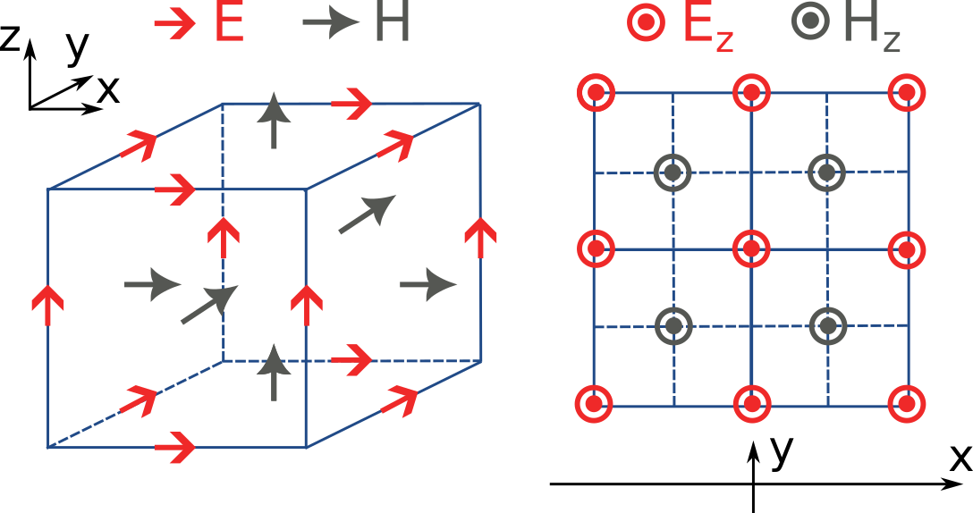
The FDTD method for electromagnetic simulations uses what is called the Yee grid, in which every field component is defined at a different spatial location, as illustrated in the figure, as well as in our FDTD video tutorial FDTD 101 videos. On the left, we show one cell of the full 3D Yee grid and where the various E and H field components live. On the right, we show a cross-section in the xy plane and the locations of the Ez and Hz fields in that plane (note that these field components are not in the same cross-section along z but rather also offset by half a cell size). This illustrates a duality between the grids on which E and H fields live, which is related to the duality between the fields themselves. There is a primal grid, shown with solid lines, and a dual grid, shown with dashed lines, with the Ez and Hz fields living at the primal/dual vertices in the xy-plane, respectively. In some literature on the FDTD method, the primal and dual grids may even be switched as the definitions are interchangeable. In Tidy3D, the primal grid is as defined by the solid lines in the figure.
When computing results that involve multiple field components, like Poynting vector, flux, or total field intensity, it is important to use fields that are defined at the same locations for best numerical accuracy. The field components thus need to be interpolated, or colocated, to some common coordinates. All this is already done under the hood when using Tidy3D in-built methods to compute such quantities. When using field data directly, Tidy3D provides several conveniences to handle this. Firstly, field monitors have a colocate option, set to True by default, which will automatically return the field data interpolated to the primal grid vertices. The data is then ready to be used directly for computing quantities derived from any combination of the field components. The colocate option can be turned off by advanced users, in which case each field component will have different coordinates as defined by the Yee grid. In some cases, this can lead to more accurate results, as discussed, for example, in the custom source
example. In that example, when using data generated by one simulation as a source in another, it is best to use the fields as recorded on the Yee grid.
Regardless of whether the colocate option is on or off for a given monitor, the data can also be easily colocated after the solver run. In principle, if colocating to locations other than the primal grid in post-processing, it is more accurate to set colocate=False in the monitor to avoid double interpolation (first to the primal grid in the
solver, then to new locations). Regardless, the following methods work for both Yee grid data and data that has already been previously colocated:
-
data_at_boundaries = sim_data.at_boundaries(monitor_name)to colocate all fields of a monitor to the Yee grid cell boundaries (i.e. the primal grid vertexes). -
data_at_centers = sim_data.at_centers(monitor_name)to colocate all fields of a monitor to the Yee grid cell centers (i.e. the dual grid vertexes). -
data_at_coords = sim_data[monitor_name].colocate(x=x_points, y=y_points, z=z_points)to colocate all fields to a custom set of coordinates. Any or all ofx,y, andzcan be supplied; if some are not, the original data coordinates are kept along that dimension.
How fine of a grid or mesh does my simulation need? How to choose grid spec?
The FDTD and other similar numerical methods will always give approximate results for a set of finite-difference equations. The accuracy of Maxwell’s equations solution for any geometry can be arbitrarily increased by using smaller and smaller values of the space and time increments. This strategy often involves increased simulation time and memory, so it is essential to consider, for your application, the desired accuracy in results so that you can run your simulations as quickly as possible. As a gold rule of thumb, ten grid points per wavelength in the highest refractive index medium should be a good starting value for the grid resolution. However, other application specificities must be considered when defining the appropriate simulation mesh, such as very thin geometries or large electric field gradients, as usually occurs, for example, in the presence of resonances, highly confined fields, or at metal-dielectric interfaces.
Tidy3D has many features that give users a simple and flexible way to build the simulation mesh. The GridSpec object enables the user to chose between an AutoGrid, a UniformGrid, or a CustomGrid, at each of the simulation x-, y-, z-direction. An example code snippet is shown below:
uniform = tidy3d.UniformGrid(dl=0.1)

custom = tidy3d.CustomGrid(dl=[0.2, 0.2, 0.1, 0.1, 0.1, 0.2, 0.2])

auto = tidy3d.AutoGrid(min_steps_per_wvl=12)

grid_spec = tidy3d.GridSpec(grid_x=uniform, grid_y=custom, grid_z=auto, wavelength=1.5)More examples of setting up the simulation mesh are available on this notebook.
In general, a good strategy is to start with the default object AutoGrid to discretize the whole simulation domain and fine-tune the mesh by increasing the grid resolution at directions or regions containing smallest geometric features or high field gradients or even relaxing the discretization along directions of invariant geometry, e.g., the propagation direction of channel waveguides. The definition of an override structure is an efficient way to improve simulation accuracy while keeping the run time small.
How to use the automatic nonuniform meshing? What steps per wavelength will be sufficient?
By default, Tidy3D configures the GridSpec object to having AutoGrid, which is an advanced meshing algorithm to automatically define a nonuniform grid in all three domain directions. The resolution of this grid is specified using the desired minimum steps per wavelength in each material (min_steps_per_wvl = 10 by default). This specification, therefore, requires a target wavelength, which can be provided directly to grid_spec or inferred from any sources present in the simulation. Detailed examples on how to set up AutoGrid are present on this notebook.
As a gold rule of thumb, the default value of 10 grid points per wavelength should be a good starting value for min_steps_per_wvl. However, other application-specific features must be considered when defining the appropriate simulation mesh, such as very thin geometries or large electric field gradients, as can usually occur, for example, in the presence of resonances, highly confined fields, or at metal-dielectric interfaces. Additional control over the mesh is obtained by the dl_min parameter, which imposes a lower bound of the grid size regardless of the structures present in the simulation, including override structures with enforced=True. This is, however, a soft bound, meaning that the actual minimal grid size might be slightly smaller. Finally, the max_scale sets the maximum ratio between two consecutive grid steps. Different grid configurations can be chosen for each direction, as illustrated below:
grid_spec = td.GridSpec(
grid_x=td.AutoGrid(min_steps_per_wvl=20,dl_min=0.01),
grid_y=td.AutoGrid(min_steps_per_wvl=15),
grid_z=td.AutoGrid(min_steps_per_wvl=10,max_scale=1.6),
wavelength=1.0,
)How can I create a uniform grid?
The most standard way to define a simulation is to use a constant grid size in each of the three directions. This can be achieved simply using tidy3d.GridSpec.uniform(dl=...) as shown below.
# Setting a uniform grid size of 0.02 microns.
sim_uniform = tidy3d.Simulation(
    size=(5, 5, 5),
    grid_spec=tidy3d.GridSpec.uniform(dl=0.02),
    medium=tidy3d.Medium(permittivity=4),
    boundary_spec=tidy3d.BoundarySpec.all_sides(boundary=tidy3d.PML()),
    run_time=1e-12,
)How can I locally refine the mesh?
In some problems, the user may want to refine the grid mesh locally around specific geometry features, such as the gap between two very close waveguides where we expect the fields to be strongest. This can be achieved by adding override_structures to the simulation grid_spec. The override structures is a list of Tidy3D structures, each with an arbitrary geometry, used exclusively for the meshing. It is added on top of any physical simulation structures. There are two types of Tidy3D structures that can be added to override_structures list. The first type defines a fictitious medium inside the override structure so that the grid size is decided by the minimum steps per wavelength in the medium. The second type is more straightforward: one can directly define the grid size along each axis inside the override structures.
Fictitious Medium
The first type is identical to the Structure object that consists of a Geometry and a Medium. The grid step in the override_structure region is decided by the minimum steps per wavelength in this medium.
# Define a "dummy" box with a refractive index 5 around the central location of a slot waveguide.
refine_box = tidy3d.Structure(
    geometry=tidy3d.Box(center=(0, 0, 0), size=(td.inf, 0.4, 0.4)),
    medium=tidy3d.Medium(permittivity=5**2),
)

# Use the box as a grid refinement structure.
sim_refined = tidy3d.Simulation(
    size=[5, 3, 3],
    grid_spec=tidy3d.GridSpec.auto(
        wavelength=1.55,
        min_steps_per_wvl=20,
        override_structures=[refine_box],
    ),
    medium=tidy3d.Medium(permittivity=1.44**2),
    structures=[wave_guide_1, wave_guide_2],
    boundary_spec=tidy3d.BoundarySpec.all_sides(boundary=tidy3d.PML()),
    run_time=1e-12,
)Override Structure
The second type is the tidy3d.MeshOverrideStructure object that consists of a Geometry, and a tuple dl specifying the grid sizes along x, y, and z-directions. We can override the grid sizes just along a few selected directions by setting the value to be None in the dl tuple along the other directions. E.g., if we only plan to refine the grid size along x-direction with grid size 0.01 $\mu$m, we can apply dl=(0.01, None, None). In the following, we override the grid size along y and z to be 15.5nm.
# Define a MeshOverrideStructure.
refine_box = tidy3d.MeshOverrideStructure(
    geometry=tidy3d.Box(center=(0, 0, 0), size=(td.inf, 0.4, 0.4)),
    dl=[None, 0.015, 0.015],
)

# Use the box as a grid refinement structure.
sim_refined = tidy3d.Simulation(
    size=[5, 3, 3],
    grid_spec=tidy3d.GridSpec.auto(
        wavelength=1.55,
        min_steps_per_wvl=20,
        override_structures=[refine_box],
    ),
    medium=tidy3d.Medium(permittivity=1.44**2),
    structures=[wave_guide_1, wave_guide_2],
    boundary_spec=tidy3d.BoundarySpec.all_sides(boundary=tidy3d.PML()),
    run_time=1e-12,
)Boundary Conditions
Which types of boundary conditions are available in Tidy3D?
Tidy3D includes the following boundary condition types: Periodic, PECBoundary, PMCBoundary, BlochBoundary, PML, StablePML, and Absorber.
How do I set the perfect matched layer (PML) boundary condition?
You should use tidy3d.PML boundary condition to enclose the simulation domain with layers of a special lossy material designed to absorb incoming waves from all angles with minimal reflection. Tidy3D uses PML boundary conditions by default, but you can also set the boundaries explicitly using the all_sides() method. For example:
# Define PML boundary conditions in all sides.
bspec = tidy3d.BoundarySpec.all_sides(boundary=tidy3d.PML())

# Alternatively, you can apply the boundary at specific directions.
# bspec = tidy3d.BoundarySpec.pml(x=True, y=True)

# Build the simulation.
sim = tidy3d.Simulation(
    center=(0, 0, 0),
    size=(10, 4, 4),
    boundary_spec=bspec,
    grid_spec=tidy3d.GridSpec.auto(min_steps_per_wvl=20, wavelength=1.55),
    structures=[waveguide],
    sources=[mode_source],
    monitors=[mode_monitor],
    run_time=1e-12,
)See this notebook for more details on setting up boundary conditions.
How do I set the perfect electric conductor (PEC) boundary condition?
You should use tidy3d.PECBoundary to enclose the simulation domain using perfect electric conductors. For example:
# Define PEC boundary conditions on all sides.
bspec = tidy3d.BoundarySpec.all_sides(boundary=tidy3d.PECBoundary())

# Alternatively, you can apply the boundary at specific directions.
# bspec = tidy3d.BoundarySpec.pec(x=True, y=True)

# Build the simulation.
sim = tidy3d.Simulation(
    center=(0, 0, 0),
    size=(10, 4, 4),
    boundary_spec=bspec,
    grid_spec=tidy3d.GridSpec.auto(min_steps_per_wvl=20, wavelength=1.55),
    structures=[waveguide],
    sources=[mode_source],
    monitors=[mode_monitor],
    run_time=1e-12,
)See this notebook for more details on setting up boundary conditions.
How do I set the perfect magnetic conductor (PMC) boundary condition?
You should use tidy3d.PMCBoundary to enclose the simulation domain using perfect magnetic conductors. For example:
# Define PML boundary conditions in all sides.
bspec = tidy3d.BoundarySpec.all_sides(boundary=tidy3d.PMCBoundary())

# Alternatively, you can apply the boundary at specific directions.
# bspec = tidy3d.BoundarySpec.pmc(x=True, y=True)

# Build the simulation.
sim = tidy3d.Simulation(
    center=(0, 0, 0),
    size=(10, 4, 4),
    boundary_spec=bspec,
    grid_spec=tidy3d.GridSpec.auto(min_steps_per_wvl=20, wavelength=1.55),
    structures=[waveguide],
    sources=[mode_source],
    monitors=[mode_monitor],
    run_time=1e-12,
)See this notebook for more details on setting up boundary conditions.
How do I set the periodic boundary condition?
# Definition of periodic boundary condition in the x and y directions.
# PML in the z-direction.
bspec = tidy3d.BoundarySpec(
    x=tidy3d.Boundary(minus=tidy3d.Periodic(), plus=tidy3d.Periodic()),
    y=tidy3d.Boundary(minus=tidy3d.Periodic(), plus=tidy3d.Periodic()),
    z=tidy3d.Boundary(minus=tidy3d.PML(), plus=tidy3d.PML()),
)

# Build the simulation.
sim = tidy3d.Simulation(
    center=(0, 0, 0),
    size=(2, 2, 10),
    boundary_spec=bspec,
    grid_spec=tidy3d.GridSpec.auto(min_steps_per_wvl=20, wavelength=1.55),
    structures=[unit_cell],
    sources=[plane_wave],
    monitors=[flux_monitor],
    run_time=1e-12,
)Details about the periodic boundary condition
x-direction along a periodic structure with period $L_x$, they must satisfy:x-direction.See this notebook for more details on setting up boundary conditions.
How do I set the Bloch boundary condition?
# Simulation size.
sim_size = (2, 2, 8)

# Plane wave source at an angle.
plane_wave = tidy3d.PlaneWave(
    center=(0, 0, 3),
    size=(tidy3d.inf, tidy3d.inf, 0),
    source_time=source_time,
    direction="-",
    pol_angle=0,
    angle_theta=np.pi / 3.0,
    angle_phi=np.pi / 6.0,
)

# Bloch boundaries.
bloch_x = tidy3d.Boundary.bloch_from_source(
  source=plane_wave,
  domain_size=sim_size[0],
  axis=0,
  medium=medium
)

bloch_y = tidy3d.Boundary.bloch_from_source(
  source=plane_wave,
  domain_size=sim_size[1],
  axis=1,
  medium=medium
)

bspec = tidy3d.BoundarySpec(x=bloch_x, y=bloch_y, z=tidy3d.Boundary.pml())

# Build the simulation.
sim = tidy3d.Simulation(
    center=(0, 0, 0),
    size=sim_size,
    boundary_spec=bspec,
    grid_spec=tidy3d.GridSpec.auto(min_steps_per_wvl=20, wavelength=1.55),
    structures=[unit_cell],
    sources=[plane_wave],
    monitors=[flux_monitor],
    run_time=1e-12,
).bloch_from_source() to automatically calculate the Bloch vector based on source, background medium, axis, and domain_size information.See this notebook for more details on setting up boundary conditions.
How do I set the Absorber boundary condition?
The tidy3d.Absorber boundary condition specifies an adiabatic absorber along a single dimension. This absorber is well-suited for dispersive materials intersecting with absorbing edges of the simulation at the expense of more layers. The example below shows how to set up an absorbing boundary.
# Define PML boundary conditions in all sides.
bspec = tidy3d.BoundarySpec.all_sides(boundary=tidy3d.Absorber(num_layers=40))

# Build the simulation.
sim = tidy3d.Simulation(
    center=(0, 0, 0),
    size=(10, 4, 4),
    boundary_spec=bspec,
    grid_spec=tidy3d.GridSpec.auto(min_steps_per_wvl=20, wavelength=1.55),
    structures=[waveguide],
    sources=[mode_source],
    monitors=[mode_monitor],
    run_time=1e-12,
)See this notebook for more details on setting up boundary conditions.
How do I specify different boundary conditions on each simulation domain edge?
# Definition different boundary conditions.
bspec = tidy3d.BoundarySpec(
    x=tidy3d.Boundary(minus=tidy3d.PECBoundary(), plus=tidy3d.PECBoundary()),
    y=tidy3d.Boundary(minus=tidy3d.Periodic(), plus=tidy3d.Periodic()),
    z=tidy3d.Boundary(minus=tidy3d.PML(), plus=tidy3d.PMCBoundary()),
)

# Build the simulation.
sim = tidy3d.Simulation(
    center=(0, 0, 0),
    size=(2, 2, 10),
    boundary_spec=bspec,
    grid_spec=tidy3d.GridSpec.auto(min_steps_per_wvl=20, wavelength=1.55),
    structures=[unit_cell],
    sources=[plane_wave],
    monitors=[flux_monitor],
    run_time=1e-12,
)See this notebook for more details on setting up boundary conditions.
Can my geometry lie within the boundary layers?
Yes. A structure that reaches an absorbing boundary should generally continue through the entire PML instead of ending inside it. An infinite size, such as tidy3d.inf, can be useful along that dimension.
Keep interfaces, corners, and other sources of strong evanescent fields away from the PML. PML absorbs propagating fields but can amplify evanescent fields and cause a simulation to diverge. Tidy3D warns when a structure is less than half a wavelength from the PML; most evanescent fields decay within that distance, although some simulations require more separation.
What is the ideal distance between the geometry and absorbing layers?
In Tidy3D, a warning will appear if the distance between a structure and the absorbing layers is smaller than half of a wavelength to prevent evanescent fields from leaking into PML. In most cases, the evanescent field will naturally die off within half a wavelength, but in some instances, a larger distance may be required. It is important to keep in mind that PML only absorbs propagating fields. PML can act as an amplification medium for evanescent fields and cause a simulation to diverge.
How do I avoid reflections from the simulation edges?
You should use tidy3d.PML boundary condition to enclose the simulation domain with layers of a special lossy material designed to absorb incoming waves from all angles with minimal reflection. Tidy3D uses PML boundary conditions by default, but you can also set the boundaries explicitly using the all_sides() method. For example:
# Define PML boundary conditions in all sides.
bspec = tidy3d.BoundarySpec.all_sides(boundary=tidy3d.PML())

# Alternatively, you can apply the boundary at specific directions.
# bspec = tidy3d.BoundarySpec.pml(x=True, y=True)

# Build the simulation.
sim = tidy3d.Simulation(
    center=(0, 0, 0),
    size=(10, 4, 4),
    boundary_spec=bspec,
    grid_spec=tidy3d.GridSpec.auto(min_steps_per_wvl=20, wavelength=1.55),
    structures=[waveguide],
    sources=[mode_source],
    monitors=[mode_monitor],
    run_time=1e-12,
)In some cases, such as when an angled structure or dispersive materials lie within the PML, use tidy3d.Absorber instead. The absorber functions similarly to PML, absorbing the outgoing radiation to mimic the infinite space. However, the absorber has a slightly higher reflection and requires a bit more computation than PML, but it is numerically much more stable.
See this notebook for more details on setting up boundary conditions.
How do I simulate periodic structures in Tidy3D?
See this notebook for more details on setting up boundary conditions.
What is The Difference Between Periodic and Bloch Boundaries?
Periodic and Bloch boundary conditions are very useful for simulating periodic structures. When using Periodic boundary conditions, the fields are registered on one edge of the simulation domain and re-injected at the opposite edge. Bloch boundary conditions are similar, but they also apply a phase correction term to the fields. In other words, Periodic boundary conditions can be considered a special case of Bloch boundaries. When a normal incident plane wave is considered, there will not be any difference between them. However, if we consider a plane wave propagating at an angle, the fields from one period to the next will not be exactly periodic and will be out of phase by some amount. The Bloch boundary condition corrects this factor. Therefore, when injecting plane waves at an angle, Bloch boundaries should be used.
Symmetry
Why is it preferable to use symmetry whenever possible?
In many Tidy3D simulations, the application of field symmetries can markedly decrease computational time and FlexCredit cost, potentially achieving reductions by factors of 1/2, 1/4, or even 1/8. Therefore, we prefer to use symmetry whenever applicable. In addition, symmetry effectively filters out unwanted light polarizations or modes.
However, correctly setting up the symmetry is essential to avoid getting incorrect results. For a more extensive discussion on symmetry, please visit the dedicated tutorial.
How do I set symmetry in Tidy3D?
To configure symmetry in your simulation, assign a tuple of integers to the symmetry parameter. This tuple defines the reflection symmetry across planes bisecting the simulation domain normal to the x-, y-, and z-axes. Each element of the tuple can be set to 0 for no symmetry, 1 for even symmetry (equivalent to ‘PMC’ symmetry), or -1 for odd symmetry (equivalent to ‘PEC’ symmetry). For example,
# Define the symmetry tuple
symmetry_tuple = (0, 1, -1)

# Build the simulation.
sim = td.Simulation(
    center=(0, 0, 0),
    size=(10, 4, 4),
    boundary_spec=tidy3d.BoundarySpec.all_sides(boundary=td.PML()),
    grid_spec=tidy3d.GridSpec.auto(min_steps_per_wvl=20, wavelength=1.55),
    structures=[waveguide],
    sources=[mode_source],
    monitors=[mode_monitor],
    run_time=1e-12,
    symmetry=symmetry_tuple,
)It is crucial to consider the vectorial nature of the electromagnetic fields when determining the appropriate symmetry value. For a more extensive discussion on symmetry, please visit the dedicated tutorial.
How do I identify the symmetry planes of my simulation?
To identify the symmetry planes in your simulation, the first step is to look for reflection symmetries in the geometry as well as the sources of your setup. If your entire simulation setup has reflection symmetry with respect to the x=0 plane, then symmetry can be applied to the x-direction. Same for the y- and z-directions. This only determines if symmetry exists but doesn’t tell us what type (even or odd) of symmetry should be applied.
Once we identify the existence of symmetry in a direction, we need to evaluate the source field. When symmetry exists, certain field components are necessarily zero at the plane of symmetry. PMC symmetry (even) corresponds to zero normal electric field and zero tangential magnetic field at the symmetry plane. PEC symmetry (odd) corresponds to zero tangential electric fields and zero normal magnetic fields at the symmetry plane. Another rule of thumb is to check if the electric field created by the source is perpendicular to the symmetry plane (odd symmetry) or parallel to the symmetry plane (even symmetry).
For example, a plane wave polarized in the y-direction propagating in the z-direction has symmetry (1, -1, 0) since the electric field is parallel to the x=0 plane and perpendicular to the y=0 plane.
For a more extensive discussion on symmetry, please visit the dedicated tutorial.
What does “odd, i.e. ‘PEC’ symmetry” mean?
PEC symmetry (odd) corresponds to zero tangential electric fields and zero normal magnetic fields at the symmetry plane.
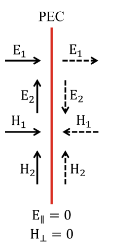
What does “even, i.e. ‘PMC’ symmetry” mean?
PMC symmetry (even) corresponds to zero normal electric field and zero tangential magnetic field at the symmetry plane.
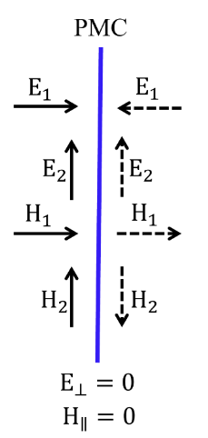
How do I filter out waveguide modes using symmetry?
Different waveguide modes process different symmetries. When we define the symmetry for the simulation, only the waveguide modes with the same symmetry can be found at the mode sources and monitors.
For example, for a rectangular strip waveguide buried in oxide with a mode source propagating in the y direction, as shown below, we can identify two symmetry planes at x=0 and z=0. All TE modes with electric fields predominantly in the x direction have symmetry (0,0,1), while all TM modes have symmetry (0,0,-1). Furthermore, even TE modes (TE0, TE2, TE4, …) have symmetry (-1,0,1) while odd TE modes (TE1, TE3, TE5, …) have symmetry (1,0,1). Even TM modes (TM0, TM2, TM4, ..) have symmetry (1,0,-1) while odd TM modes (TM1, TM3, TM5, ..) have symmetry (-1,0,-1). Therefore, by using certain symmetry, we can selectively filter out waveguide modes. Note that when the cladding and substrate materials are different or the waveguide has a nonzero sidewall angle, certain symmetry will be broken.
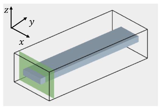
For a more extensive discussion on waveguide mode filtering using symmetry, please visit the dedicated tutorial.
Does Tidy3D support continuous and discrete rotational symmetries?
At the moment, Tidy3D does not support continuous and discrete rotational symmetries. Only mirror symmetries are supported. For more information on using symmetry to significantly reduce simulation time and cost, please refer to the tutorial Defining and using symmetries tutorial.
Mode Solver
How do I set the mode solver?
# Define the waveguide.
waveguide = tidy3d.Structure(
    geometry=tidy3d.Box(size=(tidy3d.inf, 0.5, 0.22)),
    medium=tidy3d.Medium(permittivity=3.47**2),
)

# Build a simulation object including the waveguide.
sim = tidy3d.Simulation(
    size=(10, 2.5, 1.5),
    grid_spec=tidy3d.GridSpec.auto(min_steps_per_wvl=20, wavelength=1.55),
    structures=[waveguide],
    run_time=1e-12,
    boundary_spec=tidy3d.BoundarySpec.all_sides(boundary=tidy3d.PML()),
)You can use a Box object to define the plane where you want to solve the modes. In this example, we use a plane perpendicular to the waveguide propagation axis. Symmetries are applied if they are defined in the simulation and the mode plane center sits on the simulation center. Then, use the tidy3d.ModeSpec object to specify the number of modes (num_modes), the initial effective index guess (target_neff), polarization, and other characteristics of the modes you are looking for. Make group_index_step=True to enable mode group index calculation.
# Plane we want to solve the modes.
plane = tidy3d.Box(center=(0, 0, 0), size=(0, 2.5, 1.5))

# Mode specification.
mode_spec = tidy3d.ModeSpec(
  num_modes=4,
  target_neff=3.47,
  group_index_step=True,
)Now you can create and execute the mode solver, which returns the results in a ModeSolverData object. For more details on how to set up, run, and visualize the solver results, please refer to this notebook.
from tidy3d.plugins.mode import ModeSolver
from tidy3d.plugins.mode.web import run as run_mode_solver

# Build the mode solver.
freq0 = tidy3d.C_0 / 1.55
mode_solver = ModeSolver(
  simulation=sim,
  plane=plane,
  mode_spec=mode_spec,
  freqs=[freq0],
)

# Run the server-side mode solver.
mode_data = run_mode_solver(mode_solver)If you prefer, you can run the mode solver locally with mode_data = mode_solver.solve(). Local solves do not require credits and include group-index calculation when group_index_step is enabled. By default, the local solver does not use subpixel smoothing. Installing tidy3d-extras with pip install "tidy3d[extras]" enables local subpixel averaging unless config.simulation.use_local_subpixel disables it.
How are the Output Modes Sorted?
After running the Tidy3D mode solver, the modes are returned in a ModeSolverData object. The solver finds the num_modes modes closest to target_neff. For a single-frequency solve, the default returned order is decreasing effective index. For a multi-frequency solve, ModeSortSpec.track_freq defaults to "central": the decreasing-effective-index order is exact at the central frequency, while overlap-based tracking can change the order at the other frequencies to keep each physical mode at a consistent mode index.
To group TE-like modes similarly to the old filter_pol="te" behavior, use a tidy3d.ModeSortSpec that puts modes with TE_fraction >= 0.5 first:
tidy3d.ModeSortSpec(filter_key="TE_fraction", filter_reference=0.5)
For the corresponding TM-like grouping, use the same pattern with TM_fraction:
tidy3d.ModeSortSpec(filter_key="TM_fraction", filter_reference=0.5)
The example below uses the TE-like sorting. Modes with TE_fraction >= 0.5 are returned first. Because this example solves at one frequency, modes within each group are ordered by decreasing n_eff. For a multi-frequency solve, that within-group ordering is exact only at the frequency selected by track_freq; overlap tracking can change it at the other frequencies. Modes whose polarization fraction is undefined can be ordered differently than with the legacy filter_pol option, so these settings are not exact replacements when such modes are present.
import numpy as np
import tidy3d
from tidy3d import web
from tidy3d.plugins.mode import ModeSolver

# Define the waveguide.
waveguide = tidy3d.Structure(
    geometry=tidy3d.Box(size=(tidy3d.inf, 0.5, 0.22)),
    medium=tidy3d.Medium(permittivity=3.47**2),
)

# Build a simulation object including the waveguide.
sim = tidy3d.Simulation(
    size=(10, 2.5, 1.5),
    grid_spec=tidy3d.GridSpec.auto(min_steps_per_wvl=20, wavelength=1.55),
    structures=[waveguide],
    run_time=1e-12,
    boundary_spec=tidy3d.BoundarySpec.all_sides(boundary=tidy3d.PML()),
)

# Plane where we want to solve the modes.
plane = tidy3d.Box(center=(0, 0, 0), size=(0, 2.5, 1.5))

# Group TE-like modes first, similarly to the old filter_pol="te" behavior.
mode_sort_spec = tidy3d.ModeSortSpec(
    filter_key="TE_fraction",
    filter_reference=0.5,
)

mode_spec = tidy3d.ModeSpec(
    num_modes=4,
    target_neff=3.47,
    sort_spec=mode_sort_spec,
)

# Build the mode solver.
freq0 = tidy3d.C_0 / 1.55
mode_solver = ModeSolver(
    simulation=sim,
    plane=plane,
    mode_spec=mode_spec,
    freqs=[freq0],
)

# Run the server-side mode solver.
mode_data = web.run(mode_solver, task_name="mode_sorting")

# Get the mode polarization fraction.
print("TE polarization fraction:")
print(np.asarray(mode_data.pol_fraction["te"]).squeeze())Other sorting strategies are also possible. For example, modes can be sorted by TM_fraction, mode_area, k_eff, wg_TE_fraction, or wg_TM_fraction, depending on which modal property should define the ordering.
How Do I Set the Mode Polarization?
After running the Tidy3D mode solver, the results are returned within a ModeSolverData object. The solver computes the num_modes modes closest to the given target_neff. By default, modes are sorted by decreasing effective index.
To prioritize modes with a desired polarization, use tidy3d.ModeSortSpec through ModeSpec.sort_spec. For example, to return TE-like modes first, set filter_key="TE_fraction", filter_reference=0.5. Modes with TE fraction greater than or equal to 0.5 are placed first, followed by the remaining modes. Within each group, modes use the default ordering by decreasing effective index.
The example below shows how to set the mode solver to return the TE modes first in the mode list.
import numpy as np
import tidy3d
from tidy3d.plugins.mode import ModeSolver
from tidy3d.plugins.mode.web import run as run_mode_solver

# Define the waveguide.
waveguide = tidy3d.Structure(
    geometry=tidy3d.Box(size=(tidy3d.inf, 0.5, 0.22)),
    medium=tidy3d.Medium(permittivity=3.47**2),
)

# Build a simulation object including the waveguide.
sim = tidy3d.Simulation(
    size=(10, 2.5, 1.5),
    grid_spec=tidy3d.GridSpec.auto(min_steps_per_wvl=20, wavelength=1.55),
    structures=[waveguide],
    run_time=1e-12,
    boundary_spec=tidy3d.BoundarySpec.all_sides(boundary=tidy3d.PML()),
)

# Plane where we want to solve the modes.
plane = tidy3d.Box(center=(0, 0, 0), size=(0, 2.5, 1.5))

# Mode specification.
mode_spec = tidy3d.ModeSpec(
    num_modes=4,
    target_neff=3.47,
    sort_spec=tidy3d.ModeSortSpec(
        filter_key="TE_fraction",
        filter_reference=0.5,
    ),
)

# Build the mode solver.
freq0 = tidy3d.C_0 / 1.55
mode_solver = ModeSolver(
    simulation=sim,
    plane=plane,
    mode_spec=mode_spec,
    freqs=[freq0],
)

# Run the server-side mode solver.
mode_data = run_mode_solver(mode_solver)

# Get the mode polarization fraction.
print("TE polarization fraction:")
print(np.asarray(mode_data.pol_fraction['te']).squeeze())How do I run the mode solver locally?
.solve() method. For example:from tidy3d.plugins.mode import ModeSolver
# Build the mode solver.
freq0 = tidy3d.C_0 / 1.55
mode_solver = ModeSolver(
simulation=sim,
plane=plane,
mode_spec=mode_spec,
freqs=[freq0],
)
# Run the local mode solver.
mode_data = mode_solver.solve()tidy3d-extras package is installed (pip install "tidy3d[extras]"), local subpixel averaging is automatically enabled, significantly improving accuracy. You can control this with config.simulation.use_local_subpixel: set to True to force it on, False to force it off, or leave it as None (the default) to automatically enable it when tidy3d-extras is available. For more details on how to set up, run, and visualize the solver results, please refer to this notebook.
How do I run the server-side mode solver?
from tidy3d.plugins.mode import ModeSolver
from tidy3d.plugins.mode.web import run as run_mode_solver

# Build the mode solver.
freq0 = tidy3d.C_0 / 1.55
mode_solver = ModeSolver(
  simulation=sim,
  plane=plane,
  mode_spec=mode_spec,
  freqs=[freq0],
)

# Run the server-side mode solver.
mode_data = run_mode_solver(mode_solver)To build the mode solver you need to create a simulation object and a plane where you want to calculate the modes, as well as specify the mode characteristics and frequencies of interest. The results are returned in a ModeSolverData object. For more details on how to set up, run, and visualize the solver results, please refer to this notebook.
What are the differences between running the server-side and the local mode solver?
from tidy3d.plugins.mode import ModeSolver
from tidy3d.plugins.mode.web import run as run_mode_solver

# Build the mode solver.
freq0 = tidy3d.C_0 / 1.55
mode_solver = ModeSolver(
  simulation=sim,
  plane=plane,
  mode_spec=mode_spec,
  freqs=[freq0],
)

# Run the server-side mode solver.
mode_data = run_mode_solver(mode_solver)When using the local version, the solver will run on your own computer and will not require any credits. If the tidy3d-extras package is installed (pip install "tidy3d[extras]"), the local solver will also use subpixel averaging for improved accuracy. You can control this with config.simulation.use_local_subpixel: set to True to force it on, False to force it off, or leave it as None (the default) to automatically enable it when tidy3d-extras is available. You can run the local mode solver version using:
from tidy3d.plugins.mode import ModeSolver

# Build the mode solver.
freq0 = tidy3d.C_0 / 1.55
mode_solver = ModeSolver(
  simulation=sim,
  plane=plane,
  mode_spec=mode_spec,
  freqs=[freq0],
)

# Run the local mode solver version.
mode_data = mode_solver.solve()In both cases, the results are returned in a ModeSolverData object. For more details on how to set up, run and visualize the solver results, please refer to this notebook.
Which information can I obtain from the mode solver?
to_dataframe(). We have considered a 500 x 220 nm silicon-on-insulator (SOI) waveguide operating at 1.55 $\mu$m.from tidy3d.plugins.mode import ModeSolver
from tidy3d.plugins.mode.web import run as run_mode_solver
# Define the waveguide.
waveguide = tidy3d.Structure(
geometry=tidy3d.Box(size=(tidy3d.inf, 0.5, 0.22)),
medium=tidy3d.Medium(permittivity=3.47**2),
)
# Build a simulation object including the waveguide.
sim = tidy3d.Simulation(
size=(10, 2.5, 1.5),
grid_spec=tidy3d.GridSpec.auto(min_steps_per_wvl=20, wavelength=1.55),
structures=[waveguide],
run_time=1e-12,
boundary_spec=tidy3d.BoundarySpec.all_sides(boundary=tidy3d.PML()),
)
# Plane where we want to solve the modes.
plane = tidy3d.Box(center=(0, 0, 0), size=(0, 2.5, 1.5))
# Mode specification.
mode_spec = tidy3d.ModeSpec(
num_modes=4,
target_neff=3.47,
group_index_step=True,
)
# Build the mode solver.
freq0 = tidy3d.C_0 / 1.55
mode_solver = ModeSolver(
simulation=sim,
plane=plane,
mode_spec=mode_spec,
freqs=[freq0],
)
# Run the server-side mode solver.
mode_data = run_mode_solver(mode_solver)
# Print out the results.
mode_data.to_dataframe()For more details on how to set up, run, and visualize the solver results, please refer to this notebook.
How can I get the mode solver information?
from tidy3d.plugins.mode import ModeSolver
from tidy3d.plugins.mode.web import run as run_mode_solver

# Define the waveguide.
waveguide = tidy3d.Structure(
    geometry=tidy3d.Box(size=(tidy3d.inf, 0.5, 0.22)),
    medium=tidy3d.Medium(permittivity=3.47**2),
)

# Build a simulation object including the waveguide.
sim = tidy3d.Simulation(
    size=(10, 2.5, 1.5),
    grid_spec=tidy3d.GridSpec.auto(min_steps_per_wvl=20, wavelength=1.55),
    structures=[waveguide],
    run_time=1e-12,
    boundary_spec=tidy3d.BoundarySpec.all_sides(boundary=tidy3d.PML()),
)

# Plane where we want to solve the modes.
plane = tidy3d.Box(center=(0, 0, 0), size=(0, 2.5, 1.5))

# Mode specification.
mode_spec = tidy3d.ModeSpec(
  num_modes=4,
  target_neff=3.47,
  group_index_step=True,
)

# Build the mode solver.
freq0 = tidy3d.C_0 / 1.55
mode_solver = ModeSolver(
  simulation=sim,
  plane=plane,
  mode_spec=mode_spec,
  freqs=[freq0],
)

# Run the server-side mode solver.
mode_data = run_mode_solver(mode_solver)

# Print out the results.
mode_data.to_dataframe()For more details on how to set up, run, and visualize the solver results, please refer to this notebook.
How can I get the mode field distribution?
from tidy3d.plugins.mode import ModeSolver
from tidy3d.plugins.mode.web import run as run_mode_solver

# Define the waveguide.
waveguide = tidy3d.Structure(
    geometry=tidy3d.Box(size=(tidy3d.inf, 0.5, 0.22)),
    medium=tidy3d.Medium(permittivity=3.47**2),
)

# Build a simulation object including the waveguide.
sim = tidy3d.Simulation(
    size=(10, 2.5, 1.5),
    grid_spec=tidy3d.GridSpec.auto(min_steps_per_wvl=20, wavelength=1.55),
    structures=[waveguide],
    run_time=1e-12,
    boundary_spec=tidy3d.BoundarySpec.all_sides(boundary=tidy3d.PML()),
)

# Plane where we want to solve the modes.
plane = tidy3d.Box(center=(0, 0, 0), size=(0, 2.5, 1.5))

# Mode specification.
mode_spec = tidy3d.ModeSpec(
  num_modes=1,
  target_neff=3.47,
  group_index_step=True,
)

# Build the mode solver.
freq0 = tidy3d.C_0 / 1.55
mode_solver = ModeSolver(
  simulation=sim,
  plane=plane,
  mode_spec=mode_spec,
  freqs=[freq0],
)

# Run the server-side mode solver.
mode_data = run_mode_solver(mode_solver)

# Get the mode field distribution.
Ey = mode_data.Ey.isel(mode_index=0, f=0)
Ez = mode_data.Ez.isel(mode_index=0, f=0)For more details on how to set up, run, and visualize the solver results, please refer to this notebook.
How can I plot the mode field distribution?
from tidy3d.plugins.mode import ModeSolver
from tidy3d.plugins.mode.web import run as run_mode_solver

# Define the waveguide.
waveguide = tidy3d.Structure(
    geometry=tidy3d.Box(size=(tidy3d.inf, 0.5, 0.22)),
    medium=tidy3d.Medium(permittivity=3.47**2),
)

# Build a simulation object including the waveguide.
sim = tidy3d.Simulation(
    size=(10, 2.5, 1.5),
    grid_spec=tidy3d.GridSpec.auto(min_steps_per_wvl=20, wavelength=1.55),
    structures=[waveguide],
    run_time=1e-12,
    boundary_spec=tidy3d.BoundarySpec.all_sides(boundary=tidy3d.PML()),
)

# Plane where we want to solve the modes.
plane = tidy3d.Box(center=(0, 0, 0), size=(0, 2.5, 1.5))

# Mode specification.
mode_spec = tidy3d.ModeSpec(
  num_modes=4,
  target_neff=3.47,
  group_index_step=True,
)

# Build the mode solver.
freq0 = tidy3d.C_0 / 1.55
mode_solver = ModeSolver(
  simulation=sim,
  plane=plane,
  mode_spec=mode_spec,
  freqs=[freq0],
)

# Run the server-side mode solver.
mode_data = run_mode_solver(mode_solver)

# Plot the mode field distribution.
fig, ax = plt.subplots(mode_spec.num_modes, 3, tight_layout=True, figsize=(10, 3*mode_spec.num_modes),
)
for j in range(mode_spec.num_modes):
    mode_solver.plot_field("E", "abs", mode_index=j, f=freq0, ax=ax[j, 0])
    mode_solver.plot_field("Ey", "real", mode_index=j, f=freq0, ax=ax[j, 1])
    mode_solver.plot_field("Ez", "real", mode_index=j, f=freq0, ax=ax[j, 2])
plt.show()For more details on how to set up, run, and visualize the solver results, please refer to this notebook.
How do I plot the mode effective index versus wavelength?
import numpy as np
from tidy3d.plugins.mode import ModeSolver
from tidy3d.plugins.mode.web import run as run_mode_solver

# Define the waveguide.
waveguide = tidy3d.Structure(
    geometry=tidy3d.Box(size=(tidy3d.inf, 0.5, 0.22)),
    medium=tidy3d.Medium(permittivity=3.47**2),
)

# Build a simulation object including the waveguide.
sim = tidy3d.Simulation(
    size=(10, 2.5, 1.5),
    grid_spec=tidy3d.GridSpec.auto(min_steps_per_wvl=20, wavelength=1.55),
    structures=[waveguide],
    run_time=1e-12,
    boundary_spec=tidy3d.BoundarySpec.all_sides(boundary=tidy3d.PML()),
)

# Plane where we want to solve the modes.
plane = tidy3d.Box(center=(0, 0, 0), size=(0, 2.5, 1.5))

# Mode specification.
mode_spec = tidy3d.ModeSpec(
  num_modes=4,
  target_neff=3.47,
  group_index_step=True,
)

# Build the mode solver.
wvl = np.linspace(1.5, 1.6, 51)
freqs = tidy3d.C_0 / wvl
mode_solver = ModeSolver(
  simulation=sim,
  plane=plane,
  mode_spec=mode_spec,
  freqs=freqs,
)

# Run the server-side mode solver.
mode_data = run_mode_solver(mode_solver)

# Plot the mode effective index.
n_eff = mode_data.n_eff.values.squeeze()
fig, ax = plt.subplots(1, 1, figsize=(6, 4), tight_layout=True)

for mid in range(mode_spec.num_modes):
ax.plot(wvl, n_eff[:, mid], label=(f"mode {mid}"))For more details on how to set up, run, and visualize the solver results, please refer to this notebook.
How do I plot the mode group index versus wavelength?
import numpy as np
from tidy3d.plugins.mode import ModeSolver
from tidy3d.plugins.mode.web import run as run_mode_solver

# Define the waveguide.
waveguide = tidy3d.Structure(
    geometry=tidy3d.Box(size=(tidy3d.inf, 0.5, 0.22)),
    medium=tidy3d.Medium(permittivity=3.47**2),
)

# Build a simulation object including the waveguide.
sim = tidy3d.Simulation(
    size=(10, 2.5, 1.5),
    grid_spec=tidy3d.GridSpec.auto(min_steps_per_wvl=20, wavelength=1.55),
    structures=[waveguide],
    run_time=1e-12,
    boundary_spec=tidy3d.BoundarySpec.all_sides(boundary=tidy3d.PML()),
)

# Plane where we want to solve the modes.
plane = tidy3d.Box(center=(0, 0, 0), size=(0, 2.5, 1.5))

# Mode specification.
mode_spec = tidy3d.ModeSpec(
  num_modes=4,
  target_neff=3.47,
  group_index_step=True,
)

# Build the mode solver.
wvl = np.linspace(1.5, 1.6, 51)
freqs = tidy3d.C_0 / wvl
mode_solver = ModeSolver(
  simulation=sim,
  plane=plane,
  mode_spec=mode_spec,
  freqs=freqs,
)

# Run the server-side mode solver.
mode_data = run_mode_solver(mode_solver)

# Plot the mode group index.
n_group = mode_data.n_group.values.squeeze()
fig, ax = plt.subplots(1, 1, figsize=(6, 4), tight_layout=True)

for mid in range(mode_spec.num_modes):
ax.plot(wvl, n_group[:, mid], label=(f"mode {mid}"))For more details on how to set up, run, and visualize the solver results, please refer to this notebook.
How do I calculate the mode effective area?
import numpy as np
from tidy3d.plugins.mode import ModeSolver
from tidy3d.plugins.mode.web import run as run_mode_solver

# Define the waveguide.
waveguide = tidy3d.Structure(
    geometry=tidy3d.Box(size=(tidy3d.inf, 0.5, 0.22)),
    medium=tidy3d.Medium(permittivity=3.47**2),
)

# Build a simulation object including the waveguide.
sim = tidy3d.Simulation(
    size=(10, 2.5, 1.5),
    grid_spec=tidy3d.GridSpec.auto(min_steps_per_wvl=20, wavelength=1.55),
    structures=[waveguide],
    run_time=1e-12,
    boundary_spec=tidy3d.BoundarySpec.all_sides(boundary=tidy3d.PML()),
)

# Plane where we want to solve the modes.
plane = tidy3d.Box(center=(0, 0, 0), size=(0, 2.5, 1.5))

# Mode specification.
mode_spec = tidy3d.ModeSpec(
  num_modes=4,
  target_neff=3.47,
  group_index_step=True,
)

# Build the mode solver.
freq0 = tidy3d.C_0 / 1.55
mode_solver = ModeSolver(
  simulation=sim,
  plane=plane,
  mode_spec=mode_spec,
  freqs=[freq0],
)

# Run the server-side mode solver.
mode_data = run_mode_solver(mode_solver)

# Get the mode effective area.
print("Mode effective area (um^2):")
print(np.asarray(mode_data.mode_area).squeeze())For more details on how to set up, run, and visualize the solver results, please refer to this notebook.
How do I calculate the mode polarization fraction?
import numpy as np
from tidy3d.plugins.mode import ModeSolver
from tidy3d.plugins.mode.web import run as run_mode_solver

# Define the waveguide.
waveguide = tidy3d.Structure(
    geometry=tidy3d.Box(size=(tidy3d.inf, 0.5, 0.22)),
    medium=tidy3d.Medium(permittivity=3.47**2),
)

# Build a simulation object including the waveguide.
sim = tidy3d.Simulation(
    size=(10, 2.5, 1.5),
    grid_spec=tidy3d.GridSpec.auto(min_steps_per_wvl=20, wavelength=1.55),
    structures=[waveguide],
    run_time=1e-12,
    boundary_spec=tidy3d.BoundarySpec.all_sides(boundary=tidy3d.PML()),
)

# Plane where we want to solve the modes.
plane = tidy3d.Box(center=(0, 0, 0), size=(0, 2.5, 1.5))

# Mode specification.
mode_spec = tidy3d.ModeSpec(
  num_modes=4,
  target_neff=3.47,
  group_index_step=True,
)

# Build the mode solver.
freq0 = tidy3d.C_0 / 1.55
mode_solver = ModeSolver(
  simulation=sim,
  plane=plane,
  mode_spec=mode_spec,
  freqs=[freq0],
)

# Run the server-side mode solver.
mode_data = run_mode_solver(mode_solver)

# Get the mode polarization fraction.
print("TE polarization fraction:")
print(np.asarray(mode_data.pol_fraction['te']).squeeze())

print("TM polarization fraction:")
print(np.asarray(mode_data.pol_fraction['tm']).squeeze())The TE and TM polarization fractions are defined as the field intensity along the first or the second of the two tangential axes. More precisely, if
E1andE2are the electric field components along the two tangential axes, the TE fraction is defined asintegrate(E1.abs**2) / integrate(E1.abs**2 + E2.abs**2), and theTMfraction is equal to one minus the TE fraction. The tangential axes are defined by popping the normal axis from the list ofx, y, z, so e.g.xandzfor propagation in theydirection.
For more details on how to set up, run and visualize the solver results, please refer to this notebook.
How do I calculate the waveguide mode polarization fraction?
import numpy as np
from tidy3d.plugins.mode import ModeSolver
from tidy3d.plugins.mode.web import run as run_mode_solver

# Define the waveguide.
waveguide = tidy3d.Structure(
    geometry=tidy3d.Box(size=(tidy3d.inf, 0.5, 0.22)),
    medium=tidy3d.Medium(permittivity=3.47**2),
)

# Build a simulation object including the waveguide.
sim = tidy3d.Simulation(
    size=(10, 2.5, 1.5),
    grid_spec=tidy3d.GridSpec.auto(min_steps_per_wvl=20, wavelength=1.55),
    structures=[waveguide],
    run_time=1e-12,
    boundary_spec=tidy3d.BoundarySpec.all_sides(boundary=tidy3d.PML()),
)

# Plane where we want to solve the modes.
plane = tidy3d.Box(center=(0, 0, 0), size=(0, 2.5, 1.5))

# Mode specification.
mode_spec = tidy3d.ModeSpec(
  num_modes=4,
  target_neff=3.47,
  group_index_step=True,
)

# Build the mode solver.
freq0 = tidy3d.C_0 / 1.55
mode_solver = ModeSolver(
  simulation=sim,
  plane=plane,
  mode_spec=mode_spec,
  freqs=[freq0],
)

# Run the server-side mode solver.
mode_data = run_mode_solver(mode_solver)

# Get the mode waveguide polarization fraction.
print("TE waveguide polarization fraction:")
print(np.asarray(mode_data.pol_fraction_waveguide['te']).squeeze())

print("TM waveguide polarization fraction:")
print(np.asarray(mode_data.pol_fraction_waveguide['tm']).squeeze())The TE and TM polarization fraction using the waveguide definition. If
E1andE2are the electric field components along the two tangential axes andEnis the component along the propagation direction, the TE fraction is defined as1 - integrate(En.abs**2) / integrate(E1.abs**2 + E2.abs**2 + En.abs**2), and theTMfraction is defined as1 - integrate(Hn.abs**2) / integrate(H1.abs**2 + H2.abs**2 + Hn.abs**2), withHdenoting the magnetic field components.
For more details on how to set up, run and visualize the solver results, please refer to this notebook.
Monitors
How do I set a FieldMonitor?
A FieldMonitor object records electromagnetic fields in the frequency domain. You can define a FieldMonitor object by
from tidy3d import FieldMonitor

monitor = FieldMonitor(
    center=(1,2,3),
    size=(2,2,2),
    fields=['Hx'],
    freqs=[250e12, 300e12],
    name='steady_state_monitor',
colocate=True)For details, please refer to the API reference.
How do I specify apodization?
Apodization applies a windowing function to the Fourier transform of the time-domain fields into frequency-domain ones. It can be used to truncate the beginning and/or end of the time signal, for example, to eliminate the source pulse when studying the eigenmodes of a system. Note that apodization affects the normalization of the frequency-domain fields.
To apply anodization, we first need to define an ApodizationSpec object and then add it to the monitor. For example,
# Apodization to exclude the source pulse from the frequency-domain monitors
apodization = td.ApodizationSpec(start=t_start, width=2e-13)

# Define a FieldMonitor object and add apodization to it
field_mnt = td.FieldMonitor(
    center=[0, 0, 0],
    size=[4, 2 * np.sqrt(3), 0],
    freqs=[freq0],
    name="field",
    apodization=apodization,
)How do I create field animations?
matplotlib's FuncAnimation to create the animation.phase parameter in the plot_field() function.How do I change the phase of fields obtained from frequency-domain monitors?
apply_phase() function to change the phase of fields obtained from frequency-domain monitors. For example:import numpy as np
# Run the simulation and get the data.
sim_data = tidy3d.web.run(simulation, task_name="task", path="data/data.hdf5", verbose=True)
# Get data from a field monitor.
field_data = sim_data["field_monitor"]
# Change the field phase by phi.
phi = 90 * np.pi / 180
field_phi = field_data.apply_phase(phi)How do I set a FieldTimeMonitor?
A FieldTimeMonitor object records electromagnetic fields in the time domain. You can define a FieldTimeMonitor object by
from tidy3d import FieldTimeMonitor

monitor = FieldTimeMonitor(
    center=(1,2,3),
    size=(2,2,2),
    fields=['Hx'],
    start=1e-13,
    stop=5e-13,
    interval=2,
    colocate=True,
name='movie_monitor')For details, please refer to the API reference.
How do I create a time-domain field animation?
Animations are often created from FDTD simulations to provide a more intuitive understanding of the physical phenomena being modeled. These animations can visualize the evolution of the field distribution over time, showing wave propagation, interactions, and other dynamic effects that static images cannot adequately depict.
To create a time-domain field animation, we need to capture the frames at different time instances of the simulation. This can be done by using a FieldTimeMonitor. Usually, an FDTD simulation contains a large number of time steps and grid points. Recording the field at every time step and grid point will result in a large dataset. For the purpose of making animations, this is usually unnecessary. In Tidy3D, we provide both spatial and temporal downsampling options to greatly reduce the animation data size.
Please refer to the detailed tutorial on FDTD animation creation.
How do I plot the time-domain field at a specific time?
Once a simulation with a FieldTimeMonitor is complete, the time-domain field at a specific time instance can be plotted by selecting the specific time instance and using the plot method from the data array. One example is
sim_data['movie_monitor'].Hz.sel(t=1e-13, method='nearest').plot()This line of code plots the z-component of the magnetic field at a time instance closest to 0.1 ps. Most likely, we will need to use the nearest interpolation here since the exact time instance might not be included in the result due to the finite time stepping. However, the difference is usually insignificant, so it is a very good approximation.
How do I set a FluxMonitor?
A FluxMonitor object records power flux in the frequency domain. If the monitor geometry is a 2D box, the total flux through this plane is returned, with a positive sign corresponding to power flow in the positive direction along the axis normal to the plane. If the geometry is a 3D box, the total power coming out of the box is returned by integrating the flux over all box surfaces (except the ones defined in exclude_surfaces). You can define a FluxMonitor object by
from tidy3d import FluxMonitor

monitor = FluxMonitor(
    center=(1,2,3),
    size=(2,2,0),
    freqs=[200e12, 210e12],
name='flux_monitor')For details, please refer to the API reference.
How do I calculate the Poynting vector at a specific surface?
The Poynting vector quantifies the directional energy flux of an electromagnetic field, representing the rate of energy transfer per unit area per unit time and thus characterizing the power flow within the field.
The Poynting vector at a specific plane can be calculated by first placing a FieldMonitor object at that plane to obtain the fields. Then the Poynting vector can be calculated as $\boldsymbol{S} = \boldsymbol{E} \times \boldsymbol{H}$
For example, the z-component of the Poynting vector is calculated from $E_x$, $E_y$,$H_x$, and $H_y$ as $S_z = (E_x H_y^* - E_y H_x^*)$. For time-averaged Poynting vector, we need to multiply by a factor of 0.5.
How do I integrate the Poynting vector at a specific surface?
Since the field data in Tidy3D are natively xarray.DataArray objects, the most convenient way to perform integration is by using the integrate method in xarray. For example, if we want to integrate the Poynting vector on a surface parallel to the xy plane, one needs to compute the z-component of the time-averaged Poynting vector $Sz$ and then
flux = Sz.integrate(coord=["x", "y"])This effectively achieves the same as putting a FluxMonitor object at the same plane and extracting the flux result from the monitor data.
How do I create a flux box?
A flux box can be defined by creating a FluxMonitor object with a 3D geometry. The total power coming out of the box is returned by integrating the flux over all box surfaces (except the ones defined in exclude_surfaces).
For details, please refer to the API reference.
How do I set a FluxTimeMonitor?
A FluxTimeMonitor object records power flux in the time domain. If the monitor geometry is a 2D box, the total flux through this plane is returned, with a positive sign corresponding to power flow in the positive direction along the axis normal to the plane. If the geometry is a 3D box, the total power coming out of the box is returned by integrating the flux over all box surfaces (except the ones defined in exclude_surfaces). You can define a FluxTimeMonitor object by
from tidy3d import FluxTimeMonitor

monitor = FluxTimeMonitor(
    center=(1,2,3),
    size=(2,2,0),
    start=1e-13,
    stop=5e-13,
    interval=2,
name='flux_vs_time')For details, please refer to the API reference.
How do I set a ModeMonitor?
A ModeMonitor object records complex amplitudes from the modal decomposition of fields on a plane. The amplitudes are defined as mode_solver_data.dot(recorded_field) / mode_solver_data.dot(mode_solver_data), where recorded_field is the field data recorded in the FDTD simulation at the monitor frequencies, and mode_solver_data is the mode data from the mode solver at the monitor plane. This gives the power amplitude of recorded_field carried by each mode. You can define a ModeMonitor object by
from tidy3d import ModeMonitor, ModeSpec

mode_spec = ModeSpec(num_modes=3)
monitor = ModeMonitor(
    center=(1,2,3),
    size=(2,2,0),
    freqs=[200e12, 210e12],
    mode_spec=mode_spec,
name='mode_monitor')For details, please refer to the API reference.
How do I get the coupling efficiency of a specific waveguide mode?
The coupling efficiency of a specific waveguide mode can be calculated from the mode monitor data by first extracting the complex mode amplitude and then taking the square modulus.
# extract the complex mode amplitude from the mode monitor data
amp = sim_data["mode"].amps.sel(mode_index=0, direction="+")

# compute the coupling efficiency
T = np.abs(amp)**2As an example, you can reference the waveguide Y junction case study.
How do I calculate mode overlap?
Very often we want to calculate the overlap integral of two modes to compute the coupling efficiency. This can be done conveniently using the outer_dot method such as
overlap = waveguide_mode_data_1.outer_dot(waveguide_mode_data_2)where waveguide_mode_data_1 and waveguide_mode_data_2 are ModeSolverData objects from performing the mode solving.
For advanced monitor data manipulation such as integration, please refer to the tutorial.
How do I set a ModeSolverMonitor?
A ModeSolverMonitor object stores the mode field profiles returned by the mode solver in the monitor plane. You can define a ModeSolverMonitor object by
from tidy3d import ModeSolverMonitor, ModeSpec

mode_spec = ModeSpec(num_modes=3)
monitor = ModeSolverMonitor(
    center=(1,2,3),
    size=(2,2,0),
    freqs=[200e12, 210e12],
    mode_spec=mode_spec,
name='mode_monitor')For details, please refer to the API reference.
How do I set a PermittivityMonitor?
The PermittivityMonitor records the diagonal components of the complex-valued relative permittivity tensor in the frequency domain. You can define a PermittivityMonitor object by
from tidy3d import PermittivityMonitor

monitor = PermittivityMonitor(
    center=(1,2,3),
    size=(2,2,2),
    freqs=[250e12, 300e12],
name='eps_monitor')For details, please refer to the API reference.
How do I set a FieldProjectionCartesianMonitor?
A FieldProjectionCartesianMonitor object samples electromagnetic near fields in the frequency domain and projects them on a Cartesian observation plane. The center and size fields defines where the monitor will be placed in order to record near fields, typically very close to the structure of interest. The near fields are then projected to far-field locations defined by x, y, and proj_distance, relative to the custom_origin. Here, x and y correspond to a local coordinate system where the local z axis is defined by proj_axis: which is the axis normal to this monitor. If the distance between the near and far field locations is much larger than the size of the device, one can typically set far_field_approx to True, which will make use of the far-field approximation to speed up calculations. If the projection distance is comparable to the size of the device, we recommend setting far_field_approx to False, so that the approximations are not used, and the projection is accurate even just a few wavelengths away from the near field locations. For applications where the monitor is an open surface rather than a box that encloses the device, it is advisable to pick the size of the monitor such that the recorded near fields decay to negligible values near the edges of the monitor. You can define a FieldProjectionCartesianMonitor by
from tidy3d import FieldProjectionCartesianMonitor

monitor = FieldProjectionCartesianMonitor(
    center=(1,2,3),
    size=(2,2,2),
    freqs=[250e12, 300e12],
    name='n2f_monitor',
    custom_origin=(1,2,3),
    x=[-1, 0, 1],
    y=[-2, -1, 0, 1, 2],
    proj_axis=2,
    proj_distance=5
)For details, please refer to the API reference.
How do I set a FieldProjectionAngleMonitor?
A FieldProjectionAngleMonitor object samples electromagnetic near fields in the frequency domain and projects them at given observation angles. The center and size fields defines where the monitor will be placed in order to record near fields, typically very close to the structure of interest. The near fields are then projected to far-field locations defined by phi, theta, and proj_distance, relative to the custom_origin. If the distance between the near and far field locations is much larger than the size of the device, one can typically set far_field_approx to True, which will make use of the far-field approximation to speed up calculations. If the projection distance is comparable to the size of the device, we recommend setting far_field_approx to False, so that the approximations are not used, and the projection is accurate even just a few wavelengths away from the near field locations. For applications where the monitor is an open surface rather than a box that encloses the device, it is advisable to pick the size of the monitor such that the recorded near fields decay to negligible values near the edges of the monitor. You can define a FieldProjectionAngleMonitor object by
from tidy3d import FieldProjectionAngleMonitor

monitor = FieldProjectionAngleMonitor(
    center=(1,2,3),
    size=(2,2,2),
    freqs=[250e12, 300e12],
    name='n2f_monitor',
    custom_origin=(1,2,3),
    phi=[0, np.pi/2],
    theta=np.linspace(-np.pi/2, np.pi/2, 100)
)For details, please refer to the API reference.
How do I set a FieldProjectionKSpaceMonitor?
A FieldProjectionKSpaceMonitor object samples electromagnetic near fields in the frequency domain and projects them on an observation plane defined in k-space. The center and size fields defines where the monitor will be placed in order to record near fields, typically very close to the structure of interest. The near fields are then projected to far-field locations defined in k-space by ux, uy, and proj_distance, relative to the custom_origin. Here, ux and uy are associated with a local coordinate system where the local ‘z’ axis is defined by proj_axis: which is the axis normal to this monitor. If the distance between the near and far field locations is much larger than the size of the device, one can typically set far_field_approx to True, which will make use of the far-field approximation to speed up calculations. If the projection distance is comparable to the size of the device, we recommend setting far_field_approx to False, so that the approximations are not used, and the projection is accurate even just a few wavelengths away from the near field locations. For applications where the monitor is an open surface rather than a box that encloses the device, it is advisable to pick the size of the monitor such that the recorded near fields decay to negligible values near the edges of the monitor. You can define a FieldProjectionKSpaceMonitor object by
from tidy3d import FieldProjectionKSpaceMonitor

monitor = FieldProjectionKSpaceMonitor(
    center=(1,2,3),
    size=(2,2,2),
    freqs=[250e12, 300e12],
    name='n2f_monitor',
    custom_origin=(1,2,3),
    proj_axis=2,
    ux=[0.1,0.2],
    uy=[0.3,0.4,0.5]
)For details, please refer to the API reference.
How do I set a DiffractionMonitor?
A DiffractionMonitor object uses a 2D Fourier transform to compute the diffraction amplitudes and efficiency for allowed diffraction orders. You can define a DiffractionMonitor object by
from tidy3d import DiffractionMonitor, inf

monitor = DiffractionMonitor(
    center=(1,2,3),
    size=(inf,inf,0),
    freqs=[250e12, 300e12],
    name='diffraction_monitor',
    normal_dir='+',
)For details, please refer to the API reference.
What does the FluxMonitor record?
The FluxMonitor records field data tangential $E$ and $H$ fields colocated to the cell boundaries in the monitor’s 2D plane grid. It then computes and integrates the Poynting vector, returning the real part of this integral as the flux.
where $dA$ is the area of each cell in the monitor, and the field components 1 and 2 are given depending on the monitor geometry: for $x$-normal monitors, 1 is $y$ and 2 is $z$; for $y$-normal monitors, 1 is $x$ and 2 is $z$; for $z$-normal monitors, 1 is $x$ and 2 is $y$. See the code here.
Data Visualization and Postprocessing
How do I plot an object with a spatial definition?
obj.plot(x=0) will plot the object on the x=0 plane. Note that y and z are alternatively accepted to specify other planar axes. Include the ax argument to plot to an existing axis, ie. obj.plot(y=0, ax=ax).How do I change the object plotting characteristics (facecolor, edgecolor, etc)?
plot(), for example obj.plot(x=0, edgecolor='blue', fill=False). These keyword arguments correspond to those fed to Matplotlib Patches.How do I change the global plot characteristics (title, size, etc)?
Axes, which can be manipulated, for example ax = obj.plot(x=0); ax.set_title('my_title').How do I access the data of a specific monitor?
You can access the data of a specific monitor by its name. For instance, supposing you have a field monitor and set its name to “field”, you can refer to this name after running the simulation to get the monitor’s data.
sim_data = tidy3d.web.run(simulation, task_name="task", path="data/data.hdf5", verbose=True)
field_data = sim_data["field"]
How do I interpolate the electromagnetic field data at the Yee cell centers?
To interpolate the electromagnetic fields to the Yee cell centers, you can use the method at_centers(monitor_name). For example:
# Run the simulation and get the results.
sim_data = tidy3d.web.run(simulation, task_name="task", path="data/data.hdf5", verbose=True)

# Interpolate the field at the Yee cell centers.
field_data_centered = sim_data.at_centers("monitor_name").interp(f=freq0)
By default, the electromagnetic fields are colocated to Yee grid boundaries. If you want to colocate data into custom coordinates, set
colocate=Falsein field monitors to use the raw data on the Yee grid and avoid double interpolation.
For more details on visualizing and postprocessing simulation data, see this notebook.
How do I get the monitor's data from a SimulationData object?
To get the data of a particular monitor, you can use its name. For example, if you have a field monitor and have given it the name “field”, you can refer to this name to retrieve the monitor’s data after the simulation is run.
sim_data = tidy3d.web.run(simulation, task_name="task", path="data/data.hdf5", verbose=True)
field_data = sim_data["field"]
How do I select the data at a certain coordinate value (i.e. x=0.0, f=200e12)?
The simulation data is stored as a DataArray object using the xarray package. You can think of it as a dataset where data is stored as a large multi-dimensional array (like a numpy array) and the coordinates along each of the dimensions are specified, so it is easy to work with.
You can use the sel() method to select data at certain coordinates. For example:
# Run the simulation and get the data.
sim_data = tidy3d.web.run(simulation, task_name="task", path="data/data.hdf5", verbose=True)

# Get all the data from a field monitor.
field_data = sim_data["field"]

# Get field data for a specific frequency.
field_freq = field_data.sel(f=200e14)

# Get field data for a specific position and frequency.
field_pos_freq = field_data.sel(z=0, f=200e14)You can find detailed information about simulation data visualization and postprocessing in this tutorial.
How do I get the monitor data at a certain index?
The simulation data is stored as a DataArray object using the xarray package. You can think of it as a dataset where data is stored as a large multi-dimensional array (like a numpy array) and the coordinates along each of the dimensions are specified, so it is easy to work with.
You can use the isel() method to select data at a certain coordinate index. For example:
# Run the simulation and get the data.
sim_data = tidy3d.web.run(simulation, task_name="task", path="data/data.hdf5", verbose=True)

# Get all the data from a field monitor.
field_data = sim_data["field"]

# Get field data for a specific frequency index.
field_freq_3 = field_data.isel(f=3)You can find detailed information about simulation data visualization and postprocessing in this tutorial.
How do I interpolate the monitor data at various coordinate values?
The simulation data is stored as a DataArray object using the xarray package. You can think of it as a dataset where data is stored as a large multi-dimensional array (like a numpy array) and the coordinates along each of the dimensions are specified, so it is easy to work with.
You can use the interp() method to interpolate data at certain coordinates. For example:
# Run the simulation and get the data.
sim_data = tidy3d.web.run(simulation, task_name="task", path="data/data.hdf5", verbose=True)

# Get all the data from a field monitor.
field_data = sim_data["field"]

# Interpolate field data at a specific frequency.
field_freq = field_data.interp(f=200e14)

# Interpolate field data at a specific position.
field_pos = field_data.interp(x=0, y=0, z=0)You can find detailed information about simulation data visualization and postprocessing in this tutorial.
How do I get the real part, imaginary part, or absolute value of complex-valued simulation data?
The simulation data is stored as a DataArray object using the xarray package. You can think of it as a dataset where data is stored as a large multi-dimensional array (like a numpy array) and the coordinates along each of the dimensions are specified, so it is easy to work with.
Some of the available convenience methods provided by DataArray can be used to obtain the real, imaginary, or absolute value of complex-valued simulation data. For instance:
# Run the simulation and get the data.
sim_data = tidy3d.web.run(simulation, task_name="task", path="data/data.hdf5", verbose=True)

# Get all the data from a field monitor.
field_data = sim_data["field"]

# Get the real part of Ex field component.
ex_real = field_data.Ex.real

# Get the imaginary part of Ey field component.
ey_imag = field_data.Ey.imag

# Get the absolute value of Ez field component.
ez_abs = abs(field_data.Ez)
You can find detailed information about simulation data visualization and postprocessing in this tutorial.
How do I get the raw monitor data values as a numpy array?
The simulation data is stored as a DataArray object using the xarray package. You can think of it as a dataset where data is stored as a large multi-dimensional array (like a numpy array) and the coordinates along each of the dimensions are specified, so it is easy to work with.
The example below shows how to get the raw monitor data as numpy arrays.
# Run the simulation and get the data.
sim_data = tidy3d.web.run(simulation, task_name="task", path="data/data.hdf5", verbose=True)

# Get all the data from a flux monitor.
flux_data = sim_data["flux_monitor"]

# Get the flux values as numpy arrays.
print(f"Shape of flux dataset = {flux_data.shape}\n.")
print(f"Frequencies in dataset = {flux_data.coords.values} \n.")
print(f"Flux values in dataset = {flux_data.values}\n.")You can find detailed information about simulation data visualization and postprocessing in this tutorial.
How do I get a specific field component from a FieldMonitor or FieldTimeMonitor?
Some of the available convenience methods provided by the DataArray can be used to get a specific field component from a FieldMonitor or FieldTimeMonitor. For instance:
# Run the simulation and get the data.
sim_data = tidy3d.web.run(simulation, task_name="task", path="data/data.hdf5", verbose=True)

# Get all the data from a field monitor.
field_data = sim_data["field"]

# Get the Ex field component.
ex = field_data.Ex

# Get the Hy field component.
hy = field_data.Hy
You can find detailed information about simulation data visualization and postprocessing in this tutorial.
How do I plot the monitor data as a function of one of its coordinates?
To plot the monitor data as a function of one of its coordinates, you can use mon_data.plot() if the data is already 1D. For example:
# Run the simulation and get the data.
sim_data = tidy3d.web.run(simulation, task_name="task", path="data/data.hdf5", verbose=True)

# Get data from a flux monitor.
flux_data = sim_data["flux_monitor"].flux

# Plot the flux data.
f, (ax1, ax2) = plt.subplots(1, 2, tight_layout=True, figsize=(8, 3))
flux_data.plot(ax=ax1)
ax2.plot(flux_data.f, flux_data.values)
plt.show()To select the x axis data explicitly or plot all the data on same plot, use mon_data.plot.line(x='f', ax=ax). Note that for all the plottings, if ax is not supplied, it will be created.
You can find detailed information about simulation data visualization and postprocessing in this tutorial.
How do I plot the simulation structure on top of my field plot?
You can use the plot_field() function to plot the structure on top of the simulated fields. For example:
# Run the simulation and get the data.
sim_data = tidy3d.web.run(simulation, task_name="task", path="data/data.hdf5", verbose=True)

# Plot the Ex field data and the structure.
ax = sim_data.plot_field(
  field_monitor_name="field",
  field_name="Ex",
  val='real',
  eps_alpha=0.2,
  phase=0,
)You can find detailed information about simulation data visualization and postprocessing in this tutorial.
How do I project electromagnetic near-field data to the far field?
In Tidy3D you can use field projections to obtain electromagnetic field data far away from a structure with knowledge of only near-field data. When projecting fields, geometric approximations can be invoked to allow computing fields far away from the structure quickly and with good accuracy, but in Tidy3D we can also turn these approximations off when projecting fields at intermediate distances away, which gives a lot of flexibility. These field projections are particularly useful for eliminating the need to simulate large regions of empty space around a structure.
See this tutorial for details on:
- How to compute projected fields on your local machine after a simulation is run, or on our servers during the simulation run.
- How to extract various quantities related to projected fields such as fields in different coordinate systems, power, and radar cross section.
- How, when far field approximations are used, the fields can dynamically be re-projected to new distances without having to run a new simulation.
- When geometric far field approximations should and should not be invoked, depending on the projection distance and the geometry of the structure.
- How to set up projections for finite-sized objects (e.g., scattering at a sphere) vs. thin but large-area structures (e.g., metasurfaces).
How do I export field data to zbf?
To export planar field monitor data to a Zemax beam file (.zbf), you can use mon_data.to_zbf(). For example:
# Run the simulation and get the data.
sim_data = tidy3d.web.run(simulation, task_name="task", path="data/data.hdf5", verbose=True)

# Save the data to a zbf file
ex, ey = sim_data['field_monitor'].to_zbf(
    fname='myzbf.zbf',
    background_refractive_index=1.0,
)
Detailed documentation can be found: here
How do I export Simulation data output to MATLAB format?
You can use the SimulationData.to_mat_file function to export simulation data in MATLAB format. For example:
# Run the simulation and get the data.
sim_data = tidy3d.web.run(simulation, task_name="task", path="data/data.hdf5", verbose=True)

# Export to MATLAB format.
sim_data.to_mat_file('/path/to/file/data.mat') You can find detailed information about simulation data visualization and postprocessing in this tutorial.
Scattering Matrix
How do I compute scattering matrix parameters for modeling my device?
To compute scattering matrix parameters, you need to create a base tidy3d.Simulation (without the modal sources or monitors used to compute S-parameters) and include tidy3d.plugins.smatrix.Port objects. These ports will be converted into modal sources and monitors later, so they require a mode specification and a definition of the direction that points into the system. You should also give them names to refer to later. For example:
from tidy3d.plugins.smatrix.smatrix import Port

num_modes = 1

# Port definition.
port_right_top = Port(
  center=[-5, 3, 0],
  size=[0, 4, 2],
  mode_spec=tidy3d.ModeSpec(num_modes=num_modes),
  direction="-",
  name="right_top",
)Next, add the base simulation and ports to the tidy3d.plugins.smatrix.ComponentModeler, along with the frequency of interest and a name for saving the batch of simulations that will get created later.
from tidy3d.plugins.smatrix.smatrix import ComponentModeler

modeler = ComponentModeler(
  simulation=sim,
  ports=ports,
  freqs=[freq0],
  verbose=True
)

modeler.plot_sim(z=0)With the component modeler defined, you should call it’s .solve() method to run a batch of simulations to compute the S matrix. The tool will loop through each port and create one simulation per mode index (as defined by the mode specifications), where a unique modal source is injected. Each of the ports will also be converted to mode monitors to measure the mode amplitudes and normalization.
from tidy3d.plugins.smatrix.smatrix import Port

smatrix = modeler.run(path_dir="data")The scattering matrix returned by the solve is an xr.DataArray relating the port names and mode indices. For example smatrix.loc[dict(port_in=name1, mode_index_in=mode_index1, port_out=name2, mode_index_out=mode_index_2)] gives the complex scattering matrix element.
See this tutorial for more details on computing the scattering matrix.
How do I specify a Port in the scattering matrix calculation?
To compute scattering matrix parameters, you need to create a base tidy3d.Simulation (without the modal sources or monitors used to compute S-parameters) and include tidy3d.plugins.smatrix.Port objects. These ports will be converted into modal sources and monitors later, so they require both some mode specification and a definition of the direction that points into the system. You should also give them names to refer to later. For example:
from tidy3d.plugins.smatrix.smatrix import Port

num_modes = 1

# Port definition.
port_right_top = Port(
  center=[-5, 3, 0],
  size=[0, 4, 2],
  mode_spec=tidy3d.ModeSpec(num_modes=num_modes),
  direction="-",
  name="right_top",
)How do I specify mappings between scattering matrix elements?
You can specify mappings between scattering matrix elements that you want to be equal up to a multiplicative factor. You can define these as element_mappings in the tidy3d.plugins.smatrix.ComponentModeler.
“Indices” are defined as a tuple of (port_name: str, mode_index: int)
“Elements” are defined as a tuple of output and input indices, respectively.
The element mappings are therefore defined as a tuple of (element, element, value) where the first element is set by the value of the 2nd element times the supplied value.
See this tutorial for more details on computing the scattering matrix.
Resonance Finder
How do I set the ResonanceFinder?
The tidy3d.plugins.resonance.ResonanceFinder plugin allows one to find resonances and extract their information from time domain field monitors without the necessity of waiting for the fields to decay completely. The ResonanceFinder plugin needs tidy3d.FieldTimeMonitor to record the field as a function of time. Importantly, you should start the monitors after the source pulse has decayed.
After setting up and running the simulation, you should construct a ResonanceFinder object and then call run() on the list of FieldTimeData objects. This will add up the signals from all field time monitors included in the simulation before searching for resonances.
from tidy3d.plugins.resonance import ResonanceFinder

resonance_finder = ResonanceFinder(freq_window=(190e14, 210e14))
resonance_data = resonance_finder.run(signals=sim_data.data)
resonance_data.to_dataframe()The run() method returns an xr.Dataset containing the decay rate, Q factor, amplitude, phase, and estimation error for each resonance as a function of frequency.
See this tutorial for more details on the ResonanceFinder plugin.
How do I get resonance quality factors?
To calculate low-quality factor resonances using Tidy3D, you can build and run a simulation until the electromagnetic fields fully decay to negligible values within the simulation domain. Then, you can obtain the resonance quality factor from the spectral response obtained from frequency-domain monitors.
However, when looking for long-lived resonances, the total time to the fields fully decay within the simulation domain can be extremely long. In this situation, the tidy3d.plugins.resonance.ResonanceFinder plugin allows one to find resonances and extract their information from time domain field monitors without the necessity of waiting for the fields to decay completely. The ResonanceFinder plugin needs tidy3d.FieldTimeMonitor to record the field as a function of time.
See this tutorial for more details on the ResonanceFinder plugin.
How do I calculate photonic band diagrams using the ResonanceFinder?
To calculate photonic band diagrams using Tidy3D you can excite the structure with several tidy3d.PointDipole sources and measure the response with several tidy3d.FieldTimeMonitor monitors. You should excite modes with a fixed Bloch wavevector by using tidy3d.BlochBoundary boundary conditions. Then, use the tidy3d.plugins.resonance.ResonanceFinder to find the resonant frequencies. By sweeping the Bloch wavevector, you can obtain the complete band structure of a photonic crystal structure.
This notebook shows a complete example of calculating a band diagram of a photonic crystal slab.
How do I calculate the effective mode volume?
To calculate the effective mode volume, you should include a tidy3d.FieldMonitor to record the electromagnetic fields within a box enclosing the cavity resonance. After running the simulation, you can follow this example to obtain the effective mode volume.
How to Ensure the Calculated Quality Factor is Accurate?
To calculate low-quality factor resonances using Tidy3D you can build and run a simulation until the electromagnetic fields fully decay to negligible values within the simulation domain. Then, you can obtain the resonance quality factor from the spectral response obtained from frequency-domain monitors. In this case, it is crucial to ensure the fields have fully decayed by the end of the simulation to get an accurate spectral response.
When looking for long-lived resonances, the total time to the fields fully decay within the simulation domain can be extremely long. In this situation, the tidy3d.plugins.resonance.ResonanceFinder plugin allows one to find resonances and extract information from time domain field monitors without the necessity of waiting for the fields to decay completely. To calculate accurate quality factors using the ResonanceFinder you should start the monitors after the source pulse has decayed.
In any case, a grid resolution convergence test is also essential to improve the results.
See this tutorial for more details on the ResonanceFinder plugin.
How do I calculate the Purcell factor?
You can calculate the Purcell factor from the cavity quality factor and effective mode volume using tidy3d.FieldMonitor and the tidy3d.plugins.resonance.ResonanceFinder plugin, as detailed in this tutorial.
Alternatively, you can calculate the Purcell factor as the ratio between the dipole power emitted in the final device and in the bulk semiconductor using tidy3d.FluxMonitor. Refer to this example for more details on this later approach.
Inverse Design
What is adjoint simulation?
autograd plugin allows users to take derivatives of arbitrary functions involving Tidy3D simulations through the use of the "adjoint method". The advantage of the adjoint method is that the gradients can be computed using only two FDTD simulations, the forward and the adjoint one, independent of the number of parameters. This makes it possible to perform gradient-based optimization or sensitivity analysis of devices with enormous numbers of parameters with minimal computational overhead. How many simulations are performed in adjoint calculations?
forward and the adjoint one, are performed when running inverse design optimizations using the autograd plugin.However, for broadband simulations, more than one adjoint simulation may be necessary depending on the type and number of monitors used.
-
Single-frequency differentiation
If all monitors are set to differentiate at a single frequency, only one adjoint simulation is needed per forward simulation, regardless of how many monitors are present. This works because adjoint sources can be linearly combined. -
Monitors with well-defined field profiles (e.g., ModeMonitor or DiffractionMonitor)
- Single monitor: One adjoint simulation per forward simulation is sufficient, even for broadband frequencies.
-
Multiple broadband monitors: Multiple adjoint simulations may be needed. Tidy3D automatically selects the most efficient strategy:
- Group single-frequency monitors into one adjoint simulation, or
- Run one adjoint simulation per monitor that includes all frequencies.
-
Monitors with arbitrary field profiles (e.g., FieldMonitor)
- These do not support broadband adjoint sources, so one adjoint simulation is needed per frequency.
- If multiple field monitors share the same frequency, they can be grouped into a single adjoint simulation.
Below is a summary of how the number of adjoint simulations depends on monitor type, frequency usage, and monitor count:
| Monitor Type | Frequencies | # of Monitors | # of Adjoint Simulations |
|---|---|---|---|
| Any | Single | Any | 1 per forward simulation |
| Mode / Diffraction | Multiple | 1 | 1 per forward simulation |
| Mode / Diffraction | Multiple | >1 | Depends (≤ #monitors or ≤ #frequencies) |
| Field (arbitrary) | Single | Any (same freq) | 1 |
| Field (arbitrary) | Multiple | 1 | = # of frequencies |
| Field (arbitrary) | Multiple | >1 (mixed freqs) | = # of unique frequencies |
How is the adjoint simulation billed?
Both the forward and the adjoint simulations are billed when running inverse design optimizations using the autograd plugin. That represents a significant reduction in computational cost, as the adjoint method allows one to calculate the gradient of an objective function with respect to thousands of design parameters using only two simulations in the simplest case.
The number of adjoint simulations — and thus the billing — depends on the monitor type, the number of monitors, and the number of frequencies involved:
-
Single-frequency differentiation:
If all monitors are configured to differentiate at a single frequency, only one adjoint simulation is needed per forward simulation, regardless of how many monitors are present. This is possible because the adjoint sources can be combined via linear superposition. -
Monitors with well-defined field profiles (e.g., ModeMonitor or DiffractionMonitor)
- If differentiating with respect to a single monitor, only one adjoint simulation is needed per forward simulation — even for broadband frequencies.
- If multiple broadband monitors are used, multiple adjoint simulations may be required. Tidy3D automatically chooses the most efficient strategy:
- Group monitors with a single frequency into one adjoint simulation (single-frequency case), or
- Run one simulation per monitor including all frequencies (broadband case).
-
Monitors with arbitrary field profiles (e.g., FieldMonitor)
- These do not support broadband adjoint sources, so one adjoint simulation is required per frequency.
- Multiple field monitors with the same frequency can still be grouped into a single adjoint simulation.
Each adjoint simulation typically costs approximately the same as the corresponding forward simulation. The total cost is therefore proportional to the number of adjoint simulations required.
Below is a table summarizing how the number of adjoint simulations depends on the type of monitor, the number of frequencies, and the number of monitors used in the optimization:
| Monitor Type | Frequencies | # of Monitors | # of Adjoint Simulations |
|---|---|---|---|
| Any | Single | Any | 1 per forward simulation |
| Mode / Diffraction | Multiple | 1 | 1 per forward simulation |
| Mode / Diffraction | Multiple | >1 | Depends (≤ #monitors or ≤ #frequencies) |
| Field (arbitrary) | Single | Any (same freq) | 1 |
| Field (arbitrary) | Multiple | 1 | = # of frequencies |
| Field (arbitrary) | Multiple | >1 (mixed freqs) | = # of unique frequencies |
We highly recommend watching the Inverse Design lectures if you are new to the adjoint method. You can also go through this tutorial for an introduction to the basic concepts related to automatic differentiation and adjoint optimization.
How do I set an inverse design problem?
With Tidy3D’s integration with Autograd, setting up an inverse design workflow is straightforward.
All you need to do is define a function to create the Simulation object as a function of the optimization parameters, run the simulation, post-process the data, and return the cost function. Once this function is defined, you can call autograd.value_and_grad to run the simulation and obtain the gradients.
General Workflow
-
Create a
make_simfunction
This function takes in the optimization parameters and returns aSimulationobject. -
Define a post-processing function
This function calculates the objective (cost) function from the resultingSimulationDataobject. -
Wrap it all in a single function
This wrapper receives the optimization parameters, creates and runs the simulation, applies the post-processing, and returns the objective function. -
Use
autograd.value_and_grad
Input the wrapper function intoautograd.value_and_gradto obtain both the cost function value and its derivatives. These gradients can then be used in a gradient-based optimization algorithm to guide the inverse design process.
We highly recommend watching the Inverse Design lectures if you’re new to the adjoint method. You can also explore this tutorial for an introduction to automatic differentiation and adjoint optimization.
Should I use the inverse design plugin or autograd directly?
Tidy3D offers two inverse design interfaces. The high-level invdes plugin builds the optimization for you from a design region, penalties, and an objective. The lower-level autograd integration differentiates any function you write around a Simulation. The plugin is built on top of autograd, so choosing it costs you nothing in accuracy, only in flexibility.
Start from the design problem rather than the package:
| What you are doing | Recommended interface |
|---|---|
| Topology (density-based) optimization of a design region, using the built-in filtering and projection, erosion-dilation penalty, and Adam optimizer | invdes |
| One topology design region shared by several simulations, for example one source per port |
invdes, using InverseDesignMulti
|
| Shape optimization, where design parameters move the boundaries of boxes, cylinders, or polygons | autograd |
| Level set parameterization | autograd |
| Refining a topology-optimized device into smooth contours | autograd |
| A custom objective function over the simulation data, keeping the built-in topology workflow |
invdes, using post_process_fn or metric
|
| A custom optimizer, or a parameterization the plugin does not provide | autograd |
| Differentiating with respect to sources, mediums, or a scattering matrix | autograd |
The invdes plugin currently supports topology design regions only, and AdamOptimizer is its only optimizer. Shape and level set optimizations, and any other optimizer, are written directly against autograd.
Because the plugin wraps autograd, you are not locked in. If a design outgrows the high-level interface, you can move the same physics to an autograd objective function and keep your simulation setup.
Where to start
- High-level plugin: inverse design plugin
- Autograd basics: Autograd, automatic differentiation, and adjoint optimization
- Shape optimization: inverse design optimization of a waveguide taper
- Level set optimization: parameterized level set optimization of a y-branch
- Topology to contour refinement: how to refine a topology-optimized wavelength demultiplexer
- S-matrix objective: inverse design of a waveguide crossing using S-matrix optimization
We highly recommend watching the Inverse Design lectures if you are new to the adjoint method.
What are the differences between adjoint shape, topology, and level set optimizations?
autograd plugin allows users to take derivatives of arbitrary functions involving Tidy3D simulations through the use of the "adjoint method". The advantage of the adjoint method is that the gradients can be computed with as few as two FDTD simulations, the forward and the adjoint one, independent of the number of parameters. Broadband objectives with several monitors may need more than one adjoint simulation; see how many simulations are performed in adjoint calculations. This makes it possible to do gradient-based optimization or sensitivity analysis of devices with enormous numbers of parameters with minimal computational overhead.How do I set an adjoint shape optimization?
To create an adjoint shape optimization setup, you can use parametric structures such as Box or PolySlab that are defined as functions of the optimization parameters.
Additionally, it is possible to apply operations such as rotation, translation, and boolean operations to further manipulate the geometry.
autograd.value_and_grad to compute both the objective function and the gradient with respect to the design parameters. The objective function gradients can then feed a gradient-based optimization algorithm to drive the inverse design process.How do I set an adjoint topology optimization?
To create an adjoint topology (or density-based) optimization setup, you can control the permittivity values of a CustomMedium based on the optimization design parameters.
Once the simulation is defined, you can use the web.run method to send the simulation to our servers and process the data as usual.
autograd.value_and_grad to both compute the objective function and the gradient with respect to the design parameters. The objective function gradients can then feed a gradient-based optimization algorithm to drive the inverse design process. How do I create an adjoint parameterized level set optimization?
To create an adjoint parameterized level set-based optimization setup, you should use the design parameters as the control knots of a level set surface. Then, create a CustomMedium and set the permittivity values based on the zero level isocontour obtained from the level set surface. After that, include it in a Structure object.
Once the simulation is defined, you can use the web.run method to send the simulation to our servers and process the data as usual.
autograd.value_and_grad to both compute the objective function and the gradient with respect to the design parameters. The objective function gradients can then feed a gradient-based optimization algorithm to drive the inverse design process. How do I include fabrication constraints in adjoint shape optimization?
To ensure reliable fabrication of a device, it is crucial to avoid using feature sizes below a certain radius of curvature when performing inverse design. To achieve this, you can use a penalty function that estimates the radius of curvature around each boundary vertex and applies a substantial penalty to the objective function if the value falls below the minimum radius. The code example below demonstrates how to use the tidy3d.plugins.autograd.invdes.make_curvature_penalty function.
from tidy3d.plugins.autograd import make_curvature_penalty

curvature_penalty = make_curvature_penalty(min_radius=0.15)

def penalty(params: np.ndarray) -> float:
    """Compute penalty for a set of parameters."""
    ys = get_ys(params)
    points = anp.array([xs, ys]).T
    return curvature_penalty(points)
How do I include fabrication constraints in adjoint topology optimization?
To ensure reliable fabrication of a device, it is crucial to avoid using feature sizes below a certain radius of curvature when performing inverse design. To achieve this in topology (density-based) optimization, you can use a conic density filter, which is popular in topology optimization problems, to enforce a minimum feature size specified by the filter_radius variable. Next, a hyperbolic tangent projection function can be applied to eliminate grayscale and obtain a binarized permittivity pattern. The code example below demonstrates how to apply the conic filter and the tanh projection to the design parameters before obtaining the permittivity values.
from tidy3d.plugins.autograd import make_filter_and_project, rescale

# radius of the circular filter (um) and the threshold strength
radius = 0.120
beta = 50

filter_project = make_filter_and_project(radius, lx / nx)


def get_eps(params, beta):
    """Get the permittivity values (1, eps_wg) array as a function of the parameters (0, 1)"""
    processed_params = filter_project(params, beta)
    eps = rescale(processed_params, 1, eps_wg)
    return eps


def make_input_structures(params, beta) -> List[td.Structure]:
    box = td.Box(center=(0, 0, 0), size=(lx, ly, lz))
    eps_data = get_eps(params, beta=beta).reshape((nx, ny, 1))
    custom_structure = td.Structure.from_permittivity_array(geometry=box, eps_data=eps_data)

    return [custom_structure]
How do I include fabrication constraints in adjoint level set optimization?
To ensure reliable fabrication of a device, it is crucial to avoid using feature sizes below a certain feature size when performing inverse design. To achieve this in level set optimization, you can use penalty functions to apply a substantial penalty to the objective function if the curvature and gap size values fall below a minimum feature size. This example shows how to calculate the minimum radius of curvature and the minimum gap size penalty functions using the level set surface as input.
How do I export the final inverse design structure to GDS?
Use the .to_gds_file() method of the final Simulation to export the optimized device to a GDS file. How you obtain that final Simulation depends on which inverse design API you used.
With the high-level invdes plugin, the InverseDesignResult returned by the optimizer exposes the last simulation as result.sim_last.
import tidy3d as td
import tidy3d.plugins.invdes as tdi

# Device-specific values. 'freq0' is the frequency at which the permittivity is
# evaluated. The threshold must sit between the low and high permittivity the
# design region interpolates between; the midpoint is a reasonable default.
freq0 = td.C_0 / 1.55

# 'result' is returned by 'optimizer.run()'. If the run was interrupted, reload it
# from the optimizer backup file instead:
# result = tdi.InverseDesignResult.from_file(optimizer.results_cache_fname)

eps_min, eps_max = result.design.design_region.eps_bounds
eps_threshold = 0.5 * (eps_min + eps_max)

sim_export = result.sim_last

sim_export.to_gds_file(
    fname="inverse_design.gds",
    z=0,
    frequency=freq0,
    permittivity_threshold=eps_threshold,
)
For an InverseDesignMulti optimization, result.sim_last is a dictionary keyed by the task_names of the individual designs, so select the simulation you want by its key before exporting, for example sim_export = result.sim_last["task_name"].
With the lower-level autograd workflow, rebuild the simulation from the optimized parameters using the same function you used during the optimization, then export it the same way.
# 'make_sim' is the same function used in the objective, and 'params_opt' are
# the parameters from the final optimization step.
sim_export = make_sim(params_opt)

sim_export.to_gds_file(
    fname="inverse_design.gds",
    z=0,
    frequency=freq0,
    permittivity_threshold=eps_threshold,
)
In both cases you must set a cross-sectional plane (x, y, or z) on which to evaluate the geometry, a frequency at which to evaluate the permittivity, and a permittivity_threshold that defines the shape boundary inside a CustomMedium design region. A threshold outside the range the design region interpolates between produces an empty or completely filled contour rather than the optimized device.
By default all structures are written to layer (0, 0). To separate them, pass gds_layer_dtype_map. Note that the optimized design region carries a CustomMedium built by the plugin rather than either of the endpoint media you defined, so build the map from the media actually present in the final simulation.
layer_map = {
    structure.medium: (index, 0)
    for index, structure in enumerate(sim_export.structures)
}

sim_export.to_gds_file(
    fname="inverse_design.gds",
    z=0,
    frequency=freq0,
    permittivity_threshold=eps_threshold,
    gds_layer_dtype_map=layer_map,
    gds_cell_name="DEVICE",
)
See the Export to GDS file tutorial for a detailed example of .to_gds_file() and the other GDS export functions, and the inverse design plugin tutorial for the full high-level workflow.
How Do I Use Anisotropic Medium?
The AnisotropicMedium class is supported with the autograd plugin for diagonal anisotropy and can be used directly in inverse design workflows.
The following example shows how to create an anisotropic LN medium with the extraordinary axis aligned along the z-axis:
import tidy3d as td

# Define medium components
n_e = 2.17
n_o = 2.23

medium_xx = td.Medium(permittivity=n_o**2)
medium_yy = td.Medium(permittivity=n_o**2)
medium_zz = td.Medium(permittivity=n_e**2)

# Define anisotropic medium
medium = td.AnisotropicMedium(xx=medium_xx, yy=medium_yy, zz=medium_zz)Alternatively, you can use the built-in material library, which includes several anisotropic materials. For example, to load lithium niobate:
LiNbO3 = td.material_library["LiNbO3"]["Zelmon1997"](2)How Can I Continue an Adjoint Optimization?
Using the optax library, it is possible to save and resume an adjoint optimization by recording the optimizer object state and the parameters from the last step. This allows you to either continue an ongoing optimization or extend a completed one with additional iterations.
The Parameterized level set optimization of a y-branch example illustrates this approach.
What Monitors Can Be Used in Adjoint Simulations?
For adjoint simulations, nearly all frequency-domain monitors can be used to define the objective function:
The FluxMonitor is currently not supported, but equivalent flux information can be obtained using the FieldMonitor, as demonstrated in this example.
We currently don’t support field projection monitors, such as FieldProjectionCartesianMonitor and FieldProjectionAngleMonitor. For optimizations involving far-field projections, users can use a FieldMonitor to record the near field and locally project it to the far field, as discussed in this tutorial.
Time-domain monitors are also not supported.
We highly recommend watching the Inverse Design lectures if you’re new to the adjoint method. You can also explore this tutorial for an introduction to automatic differentiation and adjoint optimization concepts.
EME
How do I run a sweep with EME?
For length sweeps, it is convenient to use a tidy3d.EMELengthSweep object, which can be passed to the sweep_spec parameter of the tidy3d.EMESimulation object. This process is demonstrated in this tutorial.
For frequency sweeps, it is sufficient to provide a list of frequencies to the freqs parameter of the tidy3d.EMESimulation object.
It is also possible to perform a sweep over the number of periods in a periodic structure using the tidy3d.EMEPeriodicitySweep object, as demonstrated in this example.
How to define the number of modes for an EME simulation?
The tidy3d.EMEModeSpec object controls how modes are computed in each EME cell. The most important parameters to tune for accuracy and performance are described below.
num_modes
It is important to use a sufficient number of modes to accurately capture the physics of the device and ensure that the simulation results are converged. The exact number of modes required depends on the characteristics of the device. For example, larger waveguides support more propagating modes and therefore require a greater number of modes to achieve accurate results.
A recommended approach is to perform a convergence sweep, where the simulation is run with increasing numbers of modes to analyze how the results converge. This can be done efficiently using tidy3d.EMEModeSweep, which sweeps over the number of modes without recomputing them. This process is demonstrated at the end of this tutorial.
num_pml
Controls the number of PML (Perfectly Matched Layer) layers added at the edges of the mode solving cross-section. Increasing num_pml is important when the structure supports leaky or radiative modes that extend beyond the simulation boundaries. If you observe that results depend on the simulation domain size, adding PML layers can help absorb those radiative components and improve accuracy.
sort_spec
Primarily used in EME for filtering and pinning modes — for example, to retain only modes of a particular polarization (te_fraction), to exclude unwanted higher-order or spurious modes from the expansion, or to pin the mode whose field energy most overlaps a specific region via the fill_fraction_box sort key combined with ModeSortSpec.bounding_box. The fill_fraction_box option is especially useful for multi-waveguide devices (splitters, couplers, directional couplers) where the supermodes of the full cross-section need to be indexed by which waveguide they primarily live in. Filtering the mode set can also improve both accuracy and performance by focusing computational effort on the modes that contribute meaningfully to device behavior.
interp_spec
Controls how modes are interpolated across frequencies in broadband simulations. This is set via the interp_spec parameter and determines the number of frequency points at which modes are explicitly solved; intermediate frequencies are interpolated. Increasing the number of interpolation points improves broadband accuracy but increases computational cost.
Other useful parameters
-
precision: Set to"double"for simulations that require high accuracy, such as bent waveguides with low expected losses. -
bend_radiusandbend_axis: Used for simulating bent waveguides. The geometry should be defined as straight; the curvature is applied analytically during mode solving. See this tutorial for details.
Checking convergence
num_modes is only one of four discretization choices that interact; in practice all four should be tested together:
-
Number of EME cells along the propagation axis. EME solves modes at the centre of each cell and treats each cell as translation-invariant, so slowly varying sections (tapers, adiabatic bends, graded transitions) are resolved by splitting them into enough cells for each to be approximately uniform. For such structures the number of cells is typically the first convergence knob — increase
num_cellsontidy3d.EMEUniformGrid(or add boundaries totidy3d.EMEExplicitGrid) until the S-matrix stops changing. -
Number of modes per cell (
num_modes).tidy3d.EMEModeSweepscans this cheaply without re-solving modes. -
Transverse simulation window plus
num_pml. The mode plane must be wide enough that guided modes decay before the edge, and radiation modes have room to resolve. -
Yee grid resolution (
grid_specontidy3d.EMESimulation). Sets the accuracy of the underlying eigenproblem in each cell.
Tighten them one at a time — many “non-converged” symptoms come from under-resolution on a different axis than the one being tuned.
Diagnostics
Invalid-mode warnings in the simulation log usually mean the transverse window or Yee grid is too coarse to support the requested num_modes, and the extra modes come back as numerical noise. Widen the simulation and/or refine the grid (and consider more num_pml) before lowering num_modes. If a physically relevant mode is filtered out because its imaginary effective index is only slightly negative, relax the filter with increasing_mode_tolerance on EMEModeSpec.
The S-matrix keeps changing even at large num_modes — add an tidy3d.EMECoefficientMonitor to record the forward (A) and backward (B) amplitudes per cell. If a handful of high-index modes carry significant power in some cell, that cell needs more modes, a finer Yee grid, or a boundary placed at a nearby discontinuity. Set EMESimulation.store_coeffs=True to keep the full internal coefficients in EMESimulationData.coeffs.
How can I simulate bent waveguides with EME?
To simulate a bent waveguide, it is necessary to define the structure as straight in the geometry. The bend is then specified using the bend_radius parameter within the tidy3d.EMEModeSpec object. In this setup, each EME cell represents a section with the given bend radius, allowing the solver to accurately account for curvature effects. When low losses are expected, it is recommended to use “double” precision in the tidy3d.EMEModeSpec object.
The EMEModeSpec.bend_medium_frame field controls how material data in bent cells is interpreted. The default bend_medium_frame="global" treats media as fixed in physical space while the bend sweeps through them, matching the global-frame convention used in FDTD. Set bend_medium_frame="co_rotating" when the material profile should bend together with the waveguide cross-section, such as a bent fiber or a CustomMedium sampled directly on the straight EME coordinates. Bent custom media are currently only supported for bend_medium_frame="co_rotating".
For isotropic bends, for media whose tensor is effectively invariant under rotation about the bend axis, or when using bend_medium_frame="co_rotating", a single bent EME cell can often represent a long constant-curvature section. For anisotropic bends with bend_medium_frame="global", however, the material orientation seen by the local mode solver generally changes with absolute bend angle. In that case, a single repeated bent cell may miss longitudinal mode evolution and the associated coupling or back-reflection. For best accuracy, split the bent region into multiple EME cells and check convergence with respect to the number of cells. For the same reason, num_reps / EMEPeriodicitySweep and some EMELengthSweep configurations are rejected at validation time for anisotropic media in bent cells with bend_medium_frame="global", since reusing modes would require re-solving at a different local tensor orientation; resolve such bends with multiple cells instead.
For a detailed example, refer to this tutorial.
How Do I Simulate a Bent Anisotropic Waveguide with EME?
How do I simulate a bent anisotropic waveguide with EME?
Unlike isotropic bends, which can be modeled with a single EME cell (see how can I simulate bent waveguides with EME), anisotropic bends require multiple EME cells and a convergence sweep over num_cells in tidy3d.EMEUniformGrid.
The reason is that in an anisotropic medium — defined with tidy3d.FullyAnisotropicMedium or tidy3d.AnisotropicMedium — the permittivity tensor is fixed in the lab frame, but the propagation direction rotates along the arc. The local eigenmodes therefore change continuously, producing polarization mixing and back-reflections. A single EME cell misses this effect and overestimates transmission. Dividing the arc into several cells in tidy3d.EMESimulation — each with its own curved eigenmode set defined via bend_radius in tidy3d.EMEModeSpec — recovers the correct result.
mode_spec = td.EMEModeSpec(
    num_modes=num_modes,
    target_neff=target_neff,
    bend_radius=radius,
    bend_axis=1,
)

eme_sim = td.EMESimulation(
    size=(np.pi * radius, plane_size[0], plane_size[1]),  # arc length along propagation axis
    center=(0, 0, 0),
    structures=[waveguide],
    medium=background_medium,
    axis=0,
    freqs=[freq0],
    eme_grid_spec=td.EMEUniformGrid(num_cells=num_cells, mode_spec=mode_spec),
    grid_spec=grid_spec,
    store_coeffs=True,
)For a complete example featuring a 180° LiNbO₃ bend, an FDTD reference simulation, and a cell-count convergence study, refer to this tutorial.
How do I set an EME simulation?
The process of setting up an EME simulation is very similar to that of an FDTD simulation. The geometry and material specifications are the same. The main difference is the need to define an eme_grid_spec, which determines the cells where the eigenmode expansions are computed.
The EME grid can be defined in several ways:
- A uniformly spaced grid using the
tidy3d.EMEUniformGridobject. This is the simplest option and is suitable when the cross-section varies smoothly along the propagation direction. The key parameter isnum_cells, which controls how many cells the region is divided into. - A custom grid using the
tidy3d.EMEExplicitGridobject. Use this when you want full control over cell boundary positions — for example, to place boundaries at junctions, transitions, or other locations where the cross-section changes abruptly. - A combination of both uniform and explicit grids using the
tidy3d.EMECompositeGridobject. This is useful for structures that have both uniform and varying sections — for example, a taper connecting two straight waveguides. You can assign a single cell to each uniform section and use a finer grid for the tapered region.
Tips for choosing the grid:
- Uniform sections (e.g. straight waveguides) only need one cell because the cross-section does not change.
- Varying sections (e.g. tapers, bends) need enough cells so that each cell is approximately uniform. Use more cells where the cross-section changes rapidly.
- Always perform a convergence test by increasing the number of cells and checking that the results (e.g. S-parameters) have stabilized.
Refer to our EME tutorial for detailed examples on how to implement the different grid configurations.
How do I run EME locally?
An tidy3d.EMESimulation can be run end-to-end on a local machine by pairing it with the local mode solver. EMESimulation.mode_simulations yields one tidy3d.ModeSimulation per EME cell, and EMESimulation.propagate turns the mode results into the device S-matrix.
Prerequisites
EMESimulation.mode_simulations is available without any extra license and returns one ModeSimulation per EME cell. Turning those mode results into an S-matrix — via EMESimulation.propagate, EMESimulation.compute_overlaps, EMESimulation.propagate_from_overlaps, or the per-element staged helpers — requires the optional tidy3d-extras package with the local_eme feature. Install with pip install "tidy3d[extras]"; see the extras plugin page for details.
One-shot
mode_data = [ms.run_local() for ms in sim.mode_simulations]
smatrix = sim.propagate(mode_data)
Cloud-parallel mode solves
Pass the per-cell ModeSimulation objects to the explicit batch API, web.run_async, as a dict keyed by cell index. It returns a mapping with those same keys, so the results can be read back in canonical EME cell order and fed to propagate:
from tidy3d import web

mode_sims = {f"cell_{i}": ms for i, ms in enumerate(sim.mode_simulations)}
results = web.run_async(mode_sims)
mode_data = [results[f"cell_{i}"] for i in range(len(mode_sims))]
smatrix = sim.propagate(mode_data)
Reusing overlaps across sweep variants
Overlap integrals dominate the cost of propagation and are sweep-invariant under tidy3d.EMELengthSweep, tidy3d.EMEModeSweep, and tidy3d.EMEPeriodicitySweep. For iterative design on the same modal basis, compute them once with EMESimulation.compute_overlaps and replay them through EMESimulation.propagate_from_overlaps:
import tidy3d as td

cell_overlaps, interface_overlaps = sim.compute_overlaps(mode_data)

# Reuse the overlaps across sweep configurations without re-solving modes.
smatrix = sim.propagate_from_overlaps(cell_overlaps, interface_overlaps)

swept = sim.updated_copy(sweep_spec=td.EMELengthSweep(scale_factors=[0.5, 1.0, 2.0]))
smatrix_swept = swept.propagate_from_overlaps(cell_overlaps, interface_overlaps)
Full staged pipeline
For finer control — for example, to checkpoint intermediates to HDF5 or run individual stages out-of-order — each pipeline element is exposed as its own method. The stage artifacts they return (EMEStageCellModes, EMEStageCellOverlap, EMEStageInterfaceOverlap, EMEStageCellSMatrix, EMEStageInterfaceSMatrix) are all HDF5-serializable, so any subset of the pipeline can be cached to disk and replayed later:
# Stage 1: per-cell mode data → validated, filtered cell-mode artifacts.
mode_data = [ms.run_local() for ms in sim.mode_simulations]
cell_modes = [sim.stage_cell_modes(md, cell_index=i) for i, md in enumerate(mode_data)]

# Stage 2: overlap integrals (per cell and per interface).
cell_overlaps = [sim.compute_cell_overlap(cm) for cm in cell_modes]
iface_overlaps = [
    sim.compute_interface_overlap(cell_modes[li], cell_modes[ri])
    for li, ri in sim.cell_index_pairs
]

# Stage 3: per-element S-matrices, then stacked device S-matrix.
cell_sms = [sim.compute_cell_smatrix(co) for co in cell_overlaps]
iface_sms = [
    sim.compute_interface_smatrix(cell_overlaps[li], cell_overlaps[ri], io)
    for (li, ri), io in zip(sim.cell_index_pairs, iface_overlaps)
]
smatrix = sim.compute_smatrix(cell_overlaps, cell_sms, iface_sms)
To express the local S-matrix in another modal basis after propagate, propagate_from_overlaps, or compute_smatrix, use EMESimulation.smatrix_in_basis with the original port mode data and the replacement modes:
smatrix_custom = sim.smatrix_in_basis(
    smatrix,
    port_modes=(mode_data[0], mode_data[-1]),
    modes2=output_modes,
)
Omit modes1 or modes2 for ports that should stay in the EME port-mode basis. For remote EME runs, use EMESimulationData.smatrix_in_basis on the returned simulation data instead.
Limitations
The local path only produces the device S-matrix. EMESimulation.monitors (such as EMEFieldMonitor, EMEModeSolverMonitor, EMECoefficientMonitor) are dropped with a warning; run the simulation through the remote backend if you need monitor data.
For broadband EME, list target frequencies in EMESimulation.freqs and control mode reuse with EMEModeSpec.interp_spec. Anisotropic media in bent cells with bend_medium_frame="global" are unsupported locally; use bend_medium_frame="co_rotating" or the remote backend.
What is EME?
The EigenMode Expansion (EME) method is a frequency-domain technique useful for simulating very long waveguide-based structures. Its main advantage is that uniform sections of the structure require only a single cell for computation, while varying sections can be efficiently approximated using a limited number of cells. This approach can significantly reduce computational costs compared to FDTD method, while delivering highly comparable results.
Key capabilities of the Tidy3D EME solver include:
- Bidirectional propagation — Computes the full bidirectional scattering matrix, accounting for reflections and backward-propagating modes at every interface.
-
Passivity and unitarity constraints — Optional constraints ensure physically meaningful scattering matrices at cell interfaces (see the
constraintparameter oftidy3d.EMESimulation). -
Bent waveguides — Simulates curved structures via
bend_radiusintidy3d.EMEModeSpec. -
Anisotropic materials — Supports diagonally anisotropic media (
tidy3d.AnisotropicMedium). -
Fast parameter sweeps — Efficiently sweeps cell lengths, number of modes, and number of periodic repetitions without recomputing modes (see
tidy3d.EMELengthSweep,tidy3d.EMEModeSweep,tidy3d.EMEPeriodicitySweep). -
Broadband frequency interpolation — Modes are interpolated across frequencies to reduce cost (see
interp_specintidy3d.EMEModeSpec). -
Diagnostics — Access mode coefficients, interface S matrices, overlaps, and propagation indices via
tidy3d.EMECoefficientMonitor.
The scattering matrix basis
The returned S-matrix is expressed in the basis of EME modes at the two ports (the boundaries of the first and last cell in the EME grid). “Mode 0” at a given port is whichever eigenmode the solver found first in the adjacent cell — typically the fundamental guided mode, but not guaranteed to be TE0 (or any fixed polarization) across a frequency or geometry sweep. To pin the ordering, configure tidy3d.ModeSortSpec on EMEModeSpec.sort_spec — for example, sort by te_fraction to prioritize TE-like modes, or use fill_fraction_box (with ModeSortSpec.bounding_box) to pin the mode whose field-energy most overlaps a specific region, which is especially useful for multi-waveguide devices like splitters or couplers. target_neff on tidy3d.EMEModeSpec can also be used to bias toward a known effective index.
To re-express the S-matrix in a different basis — for example, the modes of an individual waveguide in a splitter rather than the supermodes of the full cross-section — use EMESimulationData.smatrix_in_basis, which requires store_port_modes=True on the simulation (the default). If the simulation includes a margin of straight waveguide before and after the device, EMESimulation.port_offsets shifts each port inward along the propagation axis.
Some common application examples include MMIs, tapers and couplers, and bent waveguides.
How do I model periodic structures with EME?
To efficiently model periodic structures with the EME solver, you can use the tidy3d.EMEPeriodicitySweep object, as demonstrated in this example.
Heat
How Do I Use Heat Data in a FDTD Simulation?
The integration with a Heat and FDTD simulation is seamlessly achieved with the PerturbationMedium and Scene objects, which allow the use of the same geometry for both physics simulations. The main steps are:
- Define the PerturbationMediums and create the Scene object.
- Create the Heat simulation from the Scene object using the
from_scenemethod. - Create the Simulation object and call the method
Scene.perturbed_mediums_copy, inputting the temperature information from the Heat simulation data.
The mediums for a Heat simulation are defined using the PerturbationMedium class. This class accepts a perturbation_spec object that models the refractive index variation as a function of temperature, such as the LinearHeatPerturbation model, which represents a linear dependence of the refractive index on temperature.
The mediums are then assigned to their respective geometries and included in a Scene object. After the Heat simulation is complete, the optical simulation can be easily generated either by using Scene.perturbed_mediums_copy in combination with Simulation.from_scene, or by using the Simulation.perturbed_mediums_copy method, which automatically creates an FDTD simulation object incorporating the temperature data from the Heat simulation.
This process is illustrated in the Thermally Tuned Ring Resonator example.
How Do I Set a Heat Simulation?
The steps to set up a heat simulation are very similar to those for an FDTD simulation:
-
Create the geometry
The Scene object hosts the simulation geometry and enables easy integration with multiphysics. -
Assign materials
Materials can be defined using SolidMedium, which requires specifying heat capacity and thermal conductivity, or FluidSpec, which represents a non-simulated fluid. -
Assign boundary conditions
These can be: -
Add a heat source
Use the HeatSource object to define a volume heating source. -
Define meshing specifications
The simplest option is to use the UniformUnstructuredGrid mesh type, where you only need to specify the grid sizedl. The mesher will automatically generate a mesh that fits the structures while respecting the given resolution. For more information about meshing options, please refer to our technical article heat-solver-introduction. -
Create the simulation object
Create a HeatChargeSimulation object. -
Run the simulation
Useweb.run, just like with an FDTD simulation.
For a full walkthrough of this process, check out the HeatSolver example notebook.
How Do I Set a Heat Source?
The heat source is defined using the HeatSource object. Users can specify the volumetric heating rate, which can be uniform or spatially varying using a SpatialDataArray object. The source can be applied to any structure within the simulation domain.
In practice, one often wants to model a heater with external current applied. To model this Joule heat source, we can calculate the volumetric Joule heat generation using
$\frac{dP}{dV} = \frac{1}{\sigma}\left(\frac{I}{w_{heater}h_{heater}}\right)^2$
where $\sigma$ is the electrical conductivity of the heater material, $I$ is the applied current, and $w_{heater}$ and $h_{heater}$ are the width and thickness of the heater, respectively.
For more information, please check our Heat solver technical article.
What are the Units for Heat Simulation?
All units follow the SI system, except for length, which is defined in micrometers (µm). This is particularly important when specifying conductivity:
-
conductivity(PositiveFloat) – [units = W/(µm·K)] -
capacity(PositiveFloat) – [units = J/(kg·K)]
However, it is straightforward to define a material using SI units with the SolidMedium.from_si_units method.
Which Types of Boundary Conditions are Available?
There are three different boundary conditions available:
-
TemperatureBC:
This specifies a fixed temperature at the boundary surface. -
HeatFluxBC:
This boundary specifies heat flux normal to the boundary, which corresponds to the derivative of the temperature normal to the boundary.
$-k\frac{\partial T}{\partial n} = Q$, where $n$ is the outward normal, so a positive $Q$ extracts heat from the domain and a negative $Q$ deposits heat into it. -
ConvectionBC:
This corresponds to convective heat transfer between the domain and the surrounding environment.
$-k\frac{\partial T}{\partial n} = h (T - T_\infty)$, where $T_\infty$ is the temperature of the environment far from the surface.
For more information about the boundary conditions, please refer to our Heat solver technical article. For an example application, you can check our heat tutorial.
How Can I Set Boundary Conditions?
Boundary conditions for heat simulations are defined using the HeatChargeBoundarySpec class, which has two required fields: condition and placement.
-
condition: Specifies the boundary condition to impose. It accepts one of the following types: - TemperatureBC - HeatFluxBC - ConvectionBC -
placement: Specifies where the boundary condition should be applied. Available options include:- [StructureBoundary](https://docs.flexcompute.com/projects/tidy3d/en/latest/api/_autosummary/tidy3d.StructureBoundary.html){: .color-primary-hover} The boundary of a structure. Only the portion of the boundary not covered by subsequent structures is considered. - [StructureStructureInterface](https://docs.flexcompute.com/projects/tidy3d/en/latest/api/_autosummary/tidy3d.StructureStructureInterface.html){: .color-primary-hover} The interface between two structures. Specifically, this refers to the boundary of the succeeding structure that lies within the preceding structure. - [MediumMediumInterface](https://docs.flexcompute.com/projects/tidy3d/en/latest/api/_autosummary/tidy3d.MediumMediumInterface.html){: .color-primary-hover} The interface between two media. - [SimulationBoundary](https://docs.flexcompute.com/projects/tidy3d/en/latest/api/_autosummary/tidy3d.SimulationBoundary.html){: .color-primary-hover} The boundary of the heat simulation domain. You can specify particular surfaces using the `surfaces` field. By default, all surfaces are selected. - [StructureSimulationBoundary](https://docs.flexcompute.com/projects/tidy3d/en/latest/api/_autosummary/tidy3d.StructureSimulationBoundary.html){: .color-primary-hover} The portion of the heat simulation domain boundary that is covered by a structure. As with `StructureBoundary`, only regions not covered by subsequent structures are included.
You can check out this HeatSolver notebook for an example of how to use it in practice.
Charge
How Can I Define Doping Profile?
Doping is defined as a box with a specific doping profile and is added to a SemiconductorMedium object.
Positive doping corresponds to the N_d (number of donors) parameter of the SemiconductorMedium, while negative doping corresponds to the N_a (number of acceptors).
The doping profile can be:
-
Uniform, implemented using the
ConstantDopingobject:
import tidy3d as td

box_coords = [
    [-1, -1, -1],
    [1, 1, 1]
]

constant_box1 = td.ConstantDoping(
    center=(0, 0, 0),
    size=(2, 2, 2),
    concentration=1e18
)

constant_box2 = td.ConstantDoping.from_bounds(
    rmin=box_coords[0],
    rmax=box_coords[1],
    concentration=1e18
)-
Gaussian, implemented using the
GaussianDopingobject:
import tidy3d as td

box_coords = [
    [-1, -1, -1],
    [1, 1, 1]
]

gaussian_box1 = td.GaussianDoping(
    center=(0, 0, 0),
    size=(2, 2, 2),
    ref_con=1e15,
    concentration=1e18,
    width=0.1,
    source="xmin"
)

gaussian_box2 = td.GaussianDoping.from_bounds(
    rmin=box_coords[0],
    rmax=box_coords[1],
    ref_con=1e15,
    concentration=1e18,
    width=0.1,
    source="xmin"
)-
Arbitrary (user-defined), implemented by directly providing a
SpatialDataArrayto theN_dorN_aarguments of theSemiconductorMedium.
This approach allows defining essentially any spatial doping profile (for example, Pearson-like implantation profiles derived from fab parameters).
import tidy3d as td
import numpy as np

# Define geometry
geometry = td.Cylinder(radius=1, length=1)

# Pearson-like doping profile
def pearson_doping(z, P, R, T, S, offset=0):
    z = z - offset
    return P * (1 + ((z - R) / T)**2)**(S / 2 + 0.75) + offset

# Create coordinates
NUM_PTS = 300
rmin, rmax = geometry.bounds
x = np.linspace(rmin[0], rmax[0], NUM_PTS)
y = np.linspace(rmin[1], rmax[1], NUM_PTS)
z = np.linspace(rmin[2], rmax[2], NUM_PTS)
X, Y, Z = np.meshgrid(x, y, z)

# Mask geometry
mask = geometry.inside(X, Y, Z)

# Doping profile along z
doping_profile = pearson_doping(
    z, P=7.77e18, R=0.10384, T=0.07878, S=1.71, offset=z.min()
)

# Create SpatialDataArray
doping_values = td.SpatialDataArray(
    mask * np.tile(doping_profile, (len(x), len(y), 1)),
    coords={"x": x, "y": y, "z": z}
)The unit for the free carrier concentration is 1/$\text{cm}^3$.
It is important to note that doping boxes are additive; i.e., if two donor doping regions overlap, the total concentration will be the sum of the overlapping contributions.
Which Types of Charge Boundary Conditions are Available?
There are three boundary conditions available for Charge simulations:
1) Voltage boundary (VoltageBC), which sets a constant potential and is commonly used to model applied bias.
import tidy3d as td

voltage_source = td.DCVoltageSource(voltage=1)
voltage_bc = td.VoltageBC(source=voltage_source)Note that the voltage argument can be an list or array, in which case all voltages will be simulated.
2) Current boundary (CurrentBC), which sets a constant current and is commonly used to model a fixed current source.
import tidy3d as td

current_source = td.DCCurrentSource(current=1)
current_bc = td.CurrentBC(source=current_source)The current argument must be a float.
3) Insulating boundary (InsulatingBC), which models an insulating boundary that blocks charge flow.
import tidy3d as td
bc = td.InsulatingBC()This boundary condition is typically used to simulate surfaces or interfaces that do not allow charge to pass through.
How Can I Define the Simulation Grid?
There are two classes available for defining the grid specification:
-
- This class implements a simple uniform unstructured grid, with the grid size defined by the
dlargument. For an application example, see this example.
- This class implements a simple uniform unstructured grid, with the grid size defined by the
from tidy3d import UniformUnstructuredGrid

heat_grid = UniformUnstructuredGrid(dl=0.1)-
- This class specifies the mesh size based on the distance from material interfaces. The finer grid near interfaces is defined by the
dl_interfaceargument, while the coarser bulk grid size is set usingdl_bulk. The distances over whichdl_interfaceanddl_bulkare enforced can be controlled with thedistance_interfaceanddistance_bulkarguments, respectively. For an application example, see this example notebook.
- This class specifies the mesh size based on the distance from material interfaces. The finer grid near interfaces is defined by the
from tidy3d import DistanceUnstructuredGrid

heat_grid = DistanceUnstructuredGrid(
     dl_interface=0.1,
     dl_bulk=1,
     distance_interface=0.3,
     distance_bulk=2,
)The user can also add refinement regions to enforce a minimum grid size in a given region using the GridRefinementRegion object, or along a line using the GridRefinementLine object. An example of this can be found in our charge solver example.
What Charge Monitors are Available?
Charge simulations support the following monitors:
-
- This monitor records the electric potential ($\Phi$).
import tidy3d as td

voltage_monitor_z0 = td.SteadyPotentialMonitor(
    center=(0, 0.14, 0),
    size=(0.6, 0.3, 0),
    name="voltage_z0",
    unstructured=True,
)-
- Records the steady-state electron ($n$) and hole ($p$) concentrations.
import tidy3d as td

carrier_monitor_z0 = td.SteadyFreeCarrierMonitor(
    center=(0, 0.14, 0),
    size=(0.6, 0.3, 0),
    name="carriers_z0",
    unstructured=True,
)-
- Records the conduction and valence band energies, intrinsic Fermi level, and electron and hole quasi-Fermi levels.
-
- Records the steady electric field ($\mathbf{E}$).
-
- Records the steady current density ($\mathbf{J}$).
-
- This monitor records the small-signal capacitance within the area or volume defined by the monitor.
import tidy3d as td

capacitance_global_mnt = td.SteadyCapacitanceMonitor(
    center=(0, 0.14, 0),
    size=(td.inf, td.inf, 0),
    name="capacitance_global_mnt",
)-
- Records per-node residuals for the potential, electron-continuity, and hole-continuity equations. It also records the thermal residual when the heat solver is active. This diagnostic monitor is available with the accelerated solver.
For an application example of Charge monitors, please refer to this example.
Note that currents are naturally computed for DC isothermal simulations without the need for a monitor. They can be accessed via the charge_data.device_characteristics.steady_dc_current_voltage object, as illustrated in this example.
How Can I Define a Semiconductor Material?
A semiconductor material is specified using the MultiPhysicsMedium, by setting its charge property to a SemiconductorMedium. The required parameters for the SemiconductorMedium are:
Density of States and Band Gap Energy
-
N_c– Effective density-of-states model for the conduction band. UseConstantEffectiveDOS(N=...)for a constant value in cm⁻³. -
N_v– Effective density-of-states model for the valence band. UseConstantEffectiveDOS(N=...)for a constant value in cm⁻³. -
E_g– Band-gap model. UseConstantEnergyBandGap(eg=...)for a temperature-independent value in eV, orVarshniEnergyBandGapfor a temperature-dependent value.
Mobility Models
Mobility can be dependent on both doping and temperature, based on the Caughey-Thomas mobility model, implemented with the class CaugheyThomasMobility, or constant (implemented with the class ConstantMobilityModel.
-
mobility_n(Union[CaugheyThomasMobility,ConstantMobilityModel]) – Electron mobility model. -
mobility_p(Union[CaugheyThomasMobility,ConstantMobilityModel]) – Hole mobility model.
Electron-hole Recombination Mechanisms
Recombination mechanisms can include:
Shockley-Read-HallRadiative Recombination-
R(List) – Array containing the recombination models to be applied to the material.
Optional Arguments
-
delta_E_g– Slotboom model for band-gap narrowing -
N_a– Acceptor concentration as aSpatialDataArrayor a list/tuple of doping boxes such asConstantDoping,GaussianDoping, orCustomDoping. Values use cm⁻³. -
N_d– Donor concentration in the same supported forms asN_a.
Wrap even a single doping box in a list or tuple, for example N_d=[ConstantDoping(concentration=1e15)].
For a practical example, please refer to this example notebook.
How Do I Set a Charge Simulation?
The steps to set up a Charge simulation are very similar to those for an FDTD simulation:
-
Create the geometry
The Scene object hosts the simulation geometry and enables easy integration with multiphysics. -
Assign materials
Assign each electrical region a SemiconductorMedium, ChargeConductorMedium, or ChargeInsulatorMedium. A MultiPhysicsMedium can carry the charge medium when the same structure also participates in another physics solver. -
Assign boundary conditions
These can be: -
Add a source
A DC voltage source can be added to the VoltageBC using a DCVoltageSource object.
Similarly, a DCCurrentSource can be added to the CurrentBC boundary to define a current source. -
Define meshing specifications
The simplest option is to use the UniformUnstructuredGrid mesh type, where you only need to specify the grid sizedl. The mesher will automatically generate a mesh that fits the structures while respecting the given resolution. -
Define the simulation type
Define the simulation type via theanalysis_specof the HeatChargeSimulation object. Several analysis types are available:- SteadyChargeDCAnalysis — non-isothermal steady-state DC analysis, where the charge and heat equations are solved together.
- IsothermalSteadyChargeDCAnalysis — steady-state DC analysis at a constant temperature.
- SSACAnalysis — small-signal AC analysis (non-isothermal).
- IsothermalSSACAnalysis — small-signal AC analysis at a constant temperature.
-
Create the simulation object
Create a HeatChargeSimulation object. -
Run the simulation
Useweb.run, just like with an FDTD simulation.
For a full walkthrough of this process, check out the Charge Solver example.
How Can I Set Charge Boundary Conditions?
Boundary conditions for charge simulations are defined using the HeatChargeBoundarySpec class, which has two required fields: condition and placement.
-
condition: Specifies the boundary condition to impose. It accepts one of the following types: -
placement: Specifies where the boundary condition should be applied. Available options include:-
StructureBoundary
The boundary of a structure. Only the portion of the boundary not covered by subsequent structures is considered. -
StructureStructureInterface
The interface between two structures. Specifically, this refers to the boundary of the succeeding structure that lies within the preceding structure. -
MediumMediumInterface
The interface between two media. -
SimulationBoundary
The boundary of the charge simulation domain. You can specify particular surfaces using thesurfacesfield. By default, all surfaces are selected. -
StructureSimulationBoundary
The portion of the charge simulation domain boundary that is covered by a structure. As withStructureBoundary, only regions not covered by subsequent structures are included.
-
You can check out this Carrier injection based Mach-Zehnder modulator notebook for an example of how to use it in practice.
Web API
Web.job?
web.Job is a lightweight container that represents one simulation workflow on the Tidy3D cloud. It tracks the workflow’s server tasks, runs and loads the result, and lets you save or restore job metadata without manually handling the original simulation or task IDs.
Use Job when working with one simulation and you want to conveniently manage its execution and save or restore its state across sessions. Most simulations have one server task and expose job.task_id. Multi-step Heat and HeatCharge workflows expose their per-step IDs through job.task_ids instead.
Minimal Example
from tidy3d import web
from tidy3d.web import Job

# Create a Job from an existing simulation
job = Job(simulation=simulation, task_name="my_task", folder_name="default")

# (Optional) Estimate cost before running
est = job.estimate_cost()
print(f"Estimated max cost (FC): {est:.2f}")

# Run the workflow and load its result
sim_data = job.run(path="out/simulation.hdf5")

# Persist the job metadata for later reuse
job.to_file("data/job.json")

# Later (even in a new session), restore and load results:
job2 = Job.from_file("data/job.json")
sim_data2 = job2.load(path="data/simulation.hdf5")job.run() supports both single-step and multi-step workflows. To inspect a single-step job before it runs, call upload(), start(), and monitor() separately. For a multi-step workflow, use job.step() to advance one step at a time and inspect job.task_ids between steps.
Convenient methods
run(path) – Run the complete workflow and load its result.
step(path) – Run the next incomplete workflow step.
upload() – Upload a single-step job without running it.
start() – Start an uploaded single-step job.
monitor() – Show progress for a running single-step job until completion.
download(path) – Download results (.hdf5).
load(path) – Download and load as SimulationData.
estimate_cost(verbose=True) – Maximum FlexCredit estimate (assumes full run time).
real_cost(verbose=True) – Final billed cost.
Web.run?
The web.run function is a high-level API method for submitting simulations and supported component modelers to Flexcompute’s cloud server. It automatically uploads the input, runs it remotely, monitors progress, downloads the results, and loads them as data objects.
It accepts one supported simulation or component modeler, or a dictionary, list, tuple, or nested combination of those inputs. For multiple inputs, the returned data preserves the input container structure. To run an existing web.Batch, call Batch.run() instead.
Example
from tidy3d import web

# Submit and run the simulation
sim_data = web.run(
    simulation,
    task_name="my_task",
    path="out/sim.hdf5"
)Optional arguments:
task_name: Name shown in the web UI. If omitted, a default name is generated.
folder_name: Where to store the simulation in the web UI (default: “default”).
path: Local results file for one input, or output directory for multiple inputs.
verbose: If True, shows progress (default).
Web.get_tasks?
web.get_tasks is a function in the public tidy3d.web API that retrieves metadata about past simulation tasks from your account. It’s useful for reviewing recent runs, checking their IDs, and organizing workflows.
What does it do?
- Returns a list of dictionaries with task metadata (e.g., ID, status, name).
- Lets you specify how many tasks to fetch and in what order.
- Can filter tasks by folder name.
Example
from tidy3d import web

# Get the 5 most recent tasks from the default folder
tasks = web.get_tasks(num_tasks=5, order="new", folder="default")

for t in tasks:
print(f"Task {t['name']} (ID: {t['id']}) - Status: {t['status']}")Web.abort?
The web.abort function allows you to stop a running simulation on the server and abort any associated data processing. Note that simply stopping the Python script or killing the kernel won’t stop the simulation in the cloud.
When you call abort, the server cancels the specified simulation and returns a TaskInfo object. This object contains details about the aborted simulation, including its status, size, and credit usage. The input parameter for web.abort is the task_id, not the Simulation object. This ID is returned by the web.upload method when a simulation is created.
Example
import tidy3d.web as web

# Abort the simulation
task_info = web.abort(task_id)

print("Simulation status:", task_info.status)Web.batch?
Batch is a container for submitting, running, monitoring, and downloading multiple simulations on the Tidy3D cloud in one go. It’s similar to a web.Job, but for a whole set of simulations (FDTD, Heat/Charge, EME, Mode solver, etc.) that run in parallel.
Estimating cost
It is possible to estimate the maximum cost of the whole batch with the Batch.estimate_cost method. For more information on simulation cost, check this article.
Running a batch
The batch is run with the Batch.run(path_dir="path_dir") method, which saves a batch file that can be loaded later and returns a BatchData object.
Loading a batch
A batch can be loaded using the Batch.from_file method. If the Batch.run method was previously used, the Batch object will contain information about all executed tasks, and the BatchData object can be returned with the Batch.load method. For more information, refer to this article.
When should I use it?
- Parameter sweeps, design-of-experiments, or any workflow with many related runs in parallel.
Minimal example
import tidy3d as td
from tidy3d.web import Batch

# 1) Build your simulations (FDTD shown as example)
sim_a = td.Simulation(...)  # define as usual
sim_b = td.Simulation(...)
sims = {"run_a": sim_a, "run_b": sim_b}

# 2) Create a Batch
batch = Batch(
    simulations=sims,
    folder_name="my_sweep",
)

# (Optional) Quick cost estimate (max, assuming full run_time)
est_fc = batch.estimate_cost(verbose=True)

# 3) Run (upload+start+monitor+download as needed)
data = batch.run(path_dir="results")

# 4) Iterate over the results already downloaded by Batch.run()
for name, sim_data in data.items():
    print(name, sim_data)
    # ... analyze sim_data ...

# 5) Access final billed cost later (after runs finish)
billed_fc = batch.real_cost(verbose=True)
print("Billed FlexCredits:", billed_fc)Web.account?
web.account is a helper function that retrieves account details for the currently authenticated user. It shows your FlexCredit balance, expiration dates, and limits on daily free simulations.
Example
from tidy3d import web

# Get account information
account_info = web.account()Example output:
Current FlexCredit balance: 10.00 and expiration date: 2024-12-31 23:59:59. Remaining daily free simulations: 3.# available FlexCredit balance:
available_flexcredits = account_info.credit
# expiration date
expiration = account_info.credit_expirationWeb.estimate_cost?
web.estimate_cost returns the maximum possible FlexCredit cost of running a simulation before it starts. This helps prevent accidentally launching overly expensive simulations.
The real cost after running the simulation can be checked with Job.real_cost.
When you already have a Job, use job.estimate_cost() and job.real_cost(). These methods work for single-step and multi-step workflows. For a multi-step Heat or HeatCharge job, job.estimate_cost() estimates only the next incomplete step; run that step with job.step(), then estimate again before starting the following step. After the workflow finishes, job.real_cost() returns the total billed cost of its server tasks.
The lower-level web.estimate_cost(task_id) and web.real_cost(task_id) functions operate on one uploaded server task. Use them only when you are working directly with a task ID rather than a Job.
Example
from tidy3d import web

# Create a job
job = web.Job(simulation=sim, task_name="job_example", verbose=True)

# Estimate its maximum cost before running
estimated_cost = job.estimate_cost()
print(f"Estimated maximum cost: {estimated_cost:.3f} FlexCredits")A minimum simulation cost may apply, depending on simulation details.
The estimate is conservative: it assumes the simulation runs its full allocated time. For more information on the real cost and how to correctly estimate the simulation time, refer to this tutorial.
Td.simulationdata.from_file?
The SimulationData.from_file method allows you to load a SimulationData object directly from a locally saved file. It is a good alternative to the web.load to avoid the time of downloading the simulation from the cloud.
The file can be saved with the SimulationData.to_file method. For more details, check this tutorial.
Example
from tidy3d import SimulationData

# Load a Simulation from an HDF5 file
sim_data = SimulationData.from_file(fname="folder/sim.hdf5")Web.load?
The web.load function is a convenient utility in Tidy3D that allows you to download and load simulation results directly into a SimulationData, HeatChargeSimulationData, or ModeSolverData, depending on the simulation.
It is particularly useful for retrieving results from simulations created and run through the Tidy3D GUI or API.
Parameters
- task_id (str): Unique identifier for the simulation task (returned when uploading).
-
path (str): Local path where the results file (
.hdf5) will be saved. Default:"simulation_data.hdf5". -
replace_existing (bool): If
True, overwrites existing files at the same path.
Notes
The task_id can be obtained in the GUI under the Simulation Assets tab, or from the Action menu on the folder page.
The example below shows the basic web.load call.
Example
from tidy3d import web

sim_data = web.load(task_id, path="out/sim.hdf5", verbose=True)

# Now you can postprocess or visualize your simulation dataWeb.get_info?
The web.get_info function retrieves detailed information about a simulation.
Given a task_id (returned when you upload a simulation), get_info returns a TaskInfo object. This object includes details such as whether the task is running or completed and how many FlexCredits were consumed. It’s useful for monitoring progress or checking costs after a run.
Parameters
-
task_id (str): Unique identifier of the task on the server (returned by
web.upload). -
verbose (bool, default=True): If
True, prints progress bars and status updates. IfFalse, runs silently.
Returns
- TaskInfo: An object containing status, size, and credit information for the task.
Example
from tidy3d import web

# Get task information
info = web.get_info(task_id)

print(info.status)   # e.g., "success"
print(info.realCost) # e.g., 0.025Web.run_async?
The web.run_async function in Tidy3D allows you to submit and run multiple simulations in parallel on the server. It supports different simulation types (FDTD, Mode, HeatCharge, EME and RF) and automatically monitors and downloads the results. Ordinary batches return a web.BatchData object. When traced FDTD parameters trigger automatic differentiation, the function instead returns a dictionary mapping task names to SimulationData; traced FDTD tasks cannot be mixed with other workflow types in the same batch.
batch_results = web.run_async(simulations=sims, verbose=verbose)For virtual GPU users
Parallel web.run_async tasks do not require switching to the FlexCredit pool. Configure the virtual-GPU allocation and optional queue priority through tidy3d.config.vgpu:
tidy3d.config.vgpu.vgpu_allocation = 4
tidy3d.config.vgpu.priority = 5
batch_results = web.run_async(simulations=sims, verbose=verbose)Web.delete?
The web.delete function in Tidy3D is used to remove simulation stored on the server. This is useful for managing storage and ensuring that old or unnecessary tasks don’t take up space.
What does it do?
Given a task_id, the function deletes the corresponding simulation. You can choose to delete only the specific version of the task or all versions within the same task group.
Example
from tidy3d import web

# Delete only this version
web.delete(task_id)

# Delete all versions of the task group
web.delete(task_id, versions=True)Parameters
-
task_id (str): Unique identifier of the task on the server (returned by
web.upload). -
versions (bool, default=False):
-
False: Deletes only the task version associated with the given task_id. -
True: Deletes all versions of the task in the task group.
-
Returns
- TaskInfo: An object containing information about the task status, size, and credit usage.
Web.delete_old?
The web.delete_old function is used to automatically clean up older simulation tasks stored on the server. It helps manage storage by removing tasks that are no longer needed after a certain number of days.
What does it do?
Given a time threshold in days, the function deletes all tasks older than that age in a specified folder. This makes it easy to clear out outdated simulations without manually deleting them one by one. Be aware that deleted tasks can’t be recovered.
- int: The total number of tasks deleted.
Example
from tidy3d import web

# Delete all tasks older than 60 days in the default folder
num_deleted = web.delete_old(days_old=60)

print(f"Deleted {num_deleted} old tasks.")Parameters
- days_old (int): Minimum number of days since task creation. Tasks older than this will be deleted.
- folder_name (str, default=”default”): Folder where the deletion will occur. Only one folder can be specified at a time.
Parameter Sweep (Legacy)
How do I save or load a tidy3d.web.Batch so I can work with it later?
to_file(path) and from_file(path) methods that will export and load their metadata as JSON files. This is especially useful for loading batches for long analysis after they have run. For example, one can save the batch information to file and load the batch later if one needs to disconnect from the service while the jobs are running.# Save batch metadata.
batch.to_file("data/batch_data.json")
# Load batch metadata into a new batch.
loaded_batch = web.Batch.from_file("data/batch_data.json")
How do I submit multiple simulations?
tidy3d.web.Batch.run() to upload, run, and get the simulations results in a tidy3d.web.BatchData object. For example:# Create a dictionary including all the simulations.
sims = {"sim_1": sim_1, "sim_2": sim_2, "sim_3": sim_3}
# Build a Batch object.
batch = tidy3d.web.Batch(simulations=sims, verbose=True)
# Run all the simulations and get the results.
batch_results = batch.run(path_dir="data")# Create a dictionary including all the simulations.
sims = {"sim_1": sim_1, "sim_2": sim_2, "sim_3": sim_3}
# Run all the simulations and get the results.
batch_results = tidy3d.web.run_async(simulations=sims, path_dir="data")For the ordinary, untraced simulations above, batch_results is a tidy3d.web.BatchData object. If the inputs contain autograd-traced FDTD parameters, web.run_async instead returns a dict[str, SimulationData]; traced FDTD tasks cannot be mixed with other workflow types in the same batch. Both result types support indexed access and .items(), but the dictionary does not provide BatchData-specific helpers.
Access one result with sim_data_1 = batch_results["sim_1"], or iterate over the results:
simulation_data = []
for task_name, result in batch_results.items():
simulation_data.append(result)In this notebook, you will find a detailed example of how to run parameter sweeps.
How to load a batch result?
When a batch is created, a batch.hdf5 file will be created automatically. Users can use this file to collect all the simulation results from the batch. First, load the batch.hdf5 file by
batch = web.Batch.from_file("folder_name/batch.hdf5")Then download and load all simulations results into a BatchData object by
batch_results = batch.load(path_dir="data")Then, you can further extract the result for each simulation from batch_results.
How do I run a parameter sweep?
tidy3d.web.Batch.run() to upload, run, and get the simulations results in a tidy3d.web.BatchData object. For example:# Create a dictionary including all the simulations.
sims = {"sim_1": sim_1, "sim_2": sim_2, "sim_3": sim_3}
# Build a Batch object.
batch = tidy3d.web.Batch(simulations=sims, verbose=True)
# Run all the simulations and get the results.
batch_results = batch.run(path_dir="data")# Create a dictionary including all the simulations.
sims = {"sim_1": sim_1, "sim_2": sim_2, "sim_3": sim_3}
# Run all the simulations and get the results.
batch_results = tidy3d.web.run_async(simulations=sims, path_dir="data")For the ordinary, untraced simulations above, batch_results is a tidy3d.web.BatchData object. If the inputs contain autograd-traced FDTD parameters, web.run_async instead returns a dict[str, SimulationData]; traced FDTD tasks cannot be mixed with other workflow types in the same batch. Both result types support indexed access and .items(), but the dictionary does not provide BatchData-specific helpers.
Access one result with sim_data_1 = batch_results["sim_1"], or iterate over the results:
simulation_data = []
for task_name, result in batch_results.items():
simulation_data.append(result)In this notebook you will find a detailed example of how to run parameter sweeps.
How do I loop through tidy3d.web.BatchData without loading all of the data into memory?
sim_data_1 = batch_results["sim_1"]. Or iterating over it in a loop, as below:simulation_data = []
for task_name, result in batch_results.items():
simulation_data.append(result)So, you will get access to the tidy3d.SimulationData instances to perform your postprocessing.


 TERMS & CONDITIONS


 How the process works:
 Try this real URL to see an example: