Author: Shoumik Debnath, Bangladesh University of Engineering and Technology (BUET)
The goal of this notebook is to cross-validate a Cs3Cu2Cl5-on-SiO2 add-drop microring resonator (MRR) design that was originally simulated in an alternative FDTD solver, using Tidy3D as an independent check. The optimization step here is intentionally lightweight (2 iterations) — its purpose is to confirm that the initial design is already near-optimal, not to perform a full inverse-design sweep. The marginal improvement (~3%) supports the conclusion that the starting parameters are well-chosen.
# Setup
import matplotlib.pyplot as plt
import numpy as np
import tidy3d as td
import tidy3d.web as web

# We will get warnings about fields not adequately decayed.
# Since we are aware of this, we will suppress these warnings
td.config.logging.level = "ERROR"

# Fixed parameters (from alternative FDTD simulation + DFT-derived material model)
LAMBDA_0 = 0.636                # µm — resonance at R=10µm
FREQ_0 = td.C_0 / LAMBDA_0
FWIDTH = FREQ_0 / 20

RING_RADIUS = 10.0              # µm
RING_WIDTH = 0.6                # µm
WG_HEIGHT = 0.4                 # µm
GAP = 0.2                       # µm
BUS_WIDTH = 0.5                 # µm — from my alternative FDTD design

# Material: Cs3Cu2Cl5 at 636 nm
CS3CU2CL5 = td.Medium(permittivity=1.72**2)
SIO2 = td.Medium(permittivity=1.457**2)

# Coupler bus segments
N_SEGMENTS = 3
SEGMENT_LENGTH = 1.5            # µm each → 4.5 µm coupling zone
BUS_LENGTH = 25.0               # µm total bus length

# Width bounds for optimization
WIDTH_MIN = 0.35                # µm
WIDTH_MAX = 0.65                # µm

RUN_TIME = 15e-12               # 15 ps

print(f"λ = {LAMBDA_0*1e3:.1f} nm, R = {RING_RADIUS} µm")
print(f"Ring: {RING_WIDTH*1e3:.0f} nm, Bus: {BUS_WIDTH*1e3:.0f} nm, Gap: {GAP*1e3:.0f} nm")
print(f"Segments: {N_SEGMENTS} × {SEGMENT_LENGTH} µm")
10:06:15 EDT WARNING: Configuration found in legacy location '~/.tidy3d'.
             Consider running 'tidy3d config migrate'.
λ = 636.0 nm, R = 10.0 µm
Ring: 600 nm, Bus: 500 nm, Gap: 200 nm
Segments: 3 × 1.5 µm
NOTE ON BUS vs RING WIDTH MISMATCH
The bus waveguide (500 nm) and ring waveguide (600 nm) are separate, evanescently coupled structures separated by a 200 nm gap. The width difference is intentional: it provides control over the effective index contrast and coupling coefficient between the bus and ring modes. Because the two waveguides are physically disconnected, there is no abrupt width transition and therefore no scattering at the junction — the coupling is purely evanescent through the gap region.
# Build simulation function
def build_sim(widths, name="sim"):
    """Build full 3D MRR simulation with segmented bus coupling region."""

    # ── Ring waveguide (annulus via two cylinders) ──
    ring_outer = td.Structure(
        geometry=td.Cylinder(
            center=(0, 0, WG_HEIGHT/2),
            radius=RING_RADIUS + RING_WIDTH/2,
            length=WG_HEIGHT, axis=2,
        ),
        medium=CS3CU2CL5,
    )
    ring_inner = td.Structure(
        geometry=td.Cylinder(
            center=(0, 0, WG_HEIGHT/2),
            radius=RING_RADIUS - RING_WIDTH/2,
            length=WG_HEIGHT, axis=2,
        ),
        medium=SIO2,
    )

    # ── Bus waveguide: input (bottom) ──
    # Gap is from ring OUTER EDGE, not center
    y_bus = -(RING_RADIUS + RING_WIDTH/2 + GAP + BUS_WIDTH/2)

    structures = [ring_outer, ring_inner]

    # Left straight section
    coupling_zone = N_SEGMENTS * SEGMENT_LENGTH
    left_len = (BUS_LENGTH - coupling_zone) / 2

    structures.append(td.Structure(
        geometry=td.Box(
            center=(-BUS_LENGTH/2 + left_len/2, y_bus, WG_HEIGHT/2),
            size=(left_len, BUS_WIDTH, WG_HEIGHT),
        ),
        medium=CS3CU2CL5,
    ))

    # Coupling segments (variable width)
    x_start = -coupling_zone / 2
    for i, w in enumerate(widths):
        x_center = x_start + (i + 0.5) * SEGMENT_LENGTH
        structures.append(td.Structure(
            geometry=td.Box(
                center=(x_center, y_bus, WG_HEIGHT/2),
                size=(SEGMENT_LENGTH, w, WG_HEIGHT),
            ),
            medium=CS3CU2CL5,
        ))

    # Right section
    structures.append(td.Structure(
        geometry=td.Box(
            center=(BUS_LENGTH/2 - left_len/2, y_bus, WG_HEIGHT/2),
            size=(left_len, BUS_WIDTH, WG_HEIGHT),
        ),
        medium=CS3CU2CL5,
    ))

    # ── Drop bus waveguide (top, symmetric) ──
    y_drop = RING_RADIUS + RING_WIDTH/2 + GAP + BUS_WIDTH/2
    structures.append(td.Structure(
        geometry=td.Box(
            center=(0, y_drop, WG_HEIGHT/2),
            size=(BUS_LENGTH, BUS_WIDTH, WG_HEIGHT),
        ),
        medium=CS3CU2CL5,
    ))

    # ── Source ──
    x_src = -BUS_LENGTH/2 + 1.5
    source = td.ModeSource(
        center=(x_src, y_bus, WG_HEIGHT/2),
        size=(0, BUS_WIDTH + 0.6, WG_HEIGHT + 0.6),
        source_time=td.GaussianPulse(freq0=FREQ_0, fwidth=FWIDTH),
        direction="+",
        mode_spec=td.ModeSpec(num_modes=1),
        mode_index=0,
    )

    # ── Monitors ──
    x_thru = BUS_LENGTH/2 - 1.5

    mon_thru = td.ModeMonitor(
        center=(x_thru, y_bus, WG_HEIGHT/2),
        size=(0, BUS_WIDTH + 0.6, WG_HEIGHT + 0.6),
        freqs=[FREQ_0],
        mode_spec=td.ModeSpec(num_modes=1),
        name="thru",
    )

    mon_drop = td.ModeMonitor(
        center=(-BUS_LENGTH/2 + 1.5, y_drop, WG_HEIGHT/2),
        size=(0, BUS_WIDTH + 0.6, WG_HEIGHT + 0.6),
        freqs=[FREQ_0],
        mode_spec=td.ModeSpec(num_modes=1),
        name="drop",
    )

    buf = 1.0
    sim_size = (
        BUS_LENGTH + 2*buf,
        2*(RING_RADIUS + RING_WIDTH/2 + GAP + WIDTH_MAX) + 2*buf,
        WG_HEIGHT + 2*buf,
    )

    sim = td.Simulation(
        size=sim_size,
        center=(0, 0, WG_HEIGHT/2),
        grid_spec=td.GridSpec.auto(min_steps_per_wvl=10, wavelength=LAMBDA_0),
        structures=structures,
        sources=[source],
        monitors=[mon_thru, mon_drop],
        run_time=RUN_TIME,
        boundary_spec=td.BoundarySpec.all_sides(boundary=td.PML()),
        medium=SIO2,
        shutoff=1e-5,
    )

    return sim


def run_sim(widths, name="sim"):
    sim = build_sim(widths, name)
    data = web.run(sim, task_name=name, verbose=False)

    thru_T = np.squeeze(np.abs(data["thru"].amps.sel(mode_index=0, direction="+").values)**2)
    drop_T = np.squeeze(np.abs(data["drop"].amps.sel(mode_index=0, direction="-").values)**2)

    return {"thru": thru_T, "drop": drop_T, "sim": sim}
# Run baseline
print("Running baseline (uniform bus width)...")
widths_baseline = np.ones(N_SEGMENTS) * BUS_WIDTH
result_base = run_sim(widths_baseline, "baseline")
print(f"\n Through: {result_base['thru']:.4f}")
print(f" Drop: {result_base['drop']:.4f}")
print(f" τ² + κ² = {result_base['thru'] + result_base['drop']:.4f}")
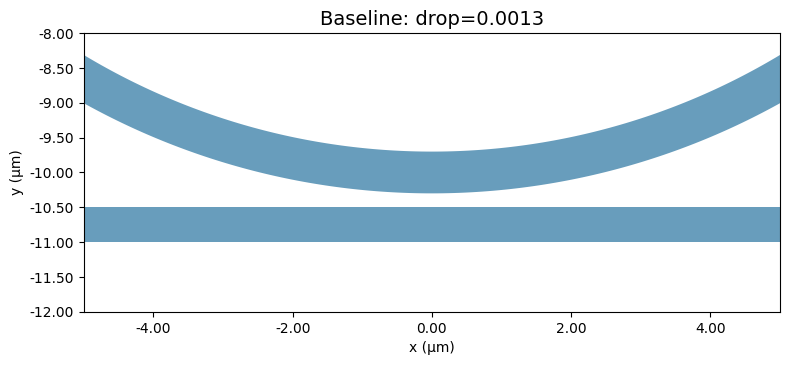
# Plot
fig, ax = plt.subplots(figsize=(8, 8))
result_base["sim"].plot(z=WG_HEIGHT/2, ax=ax)
ax.set_title(f"Baseline: drop={result_base['drop']:.4f}", fontsize=14)
ax.set_xlim(-5, 5)
ax.set_ylim(-(RING_RADIUS + 2), -(RING_RADIUS - 2))
plt.tight_layout()
plt.show()
Running baseline (uniform bus width)...

  Through: 0.9927
  Drop:    0.0013
  τ² + κ² = 0.9940
# Optimization (numerical gradient, 2 iterations)
# Cost: 3 segments × 2 perturbations × 2 iters + 2 evals = 16 sims

def objective(widths, name):
    r = run_sim(widths, name)
    # Maximize drop coupling
    return r["drop"], r

def numerical_gradient(widths, iteration, eps=0.015):
    grad = np.zeros(len(widths))
    for i in range(len(widths)):
        wp = widths.copy(); wp[i] += eps
        wm = widths.copy(); wm[i] -= eps
        fp, _ = objective(wp, f"i{iteration}_p{i}")
        fm, _ = objective(wm, f"i{iteration}_m{i}")
        grad[i] = (fp - fm) / (2 * eps)
    return grad

# Adam optimizer (pure numpy)
class Adam:
    def __init__(self, lr=0.015):
        self.lr = lr
        self.m = self.v = None
        self.t = 0
    def step(self, x, grad):
        if self.m is None:
            self.m = np.zeros_like(x)
            self.v = np.zeros_like(x)
        self.t += 1
        self.m = 0.9*self.m + 0.1*grad
        self.v = 0.999*self.v + 0.001*grad**2
        mh = self.m / (1 - 0.9**self.t)
        vh = self.v / (1 - 0.999**self.t)
        return x + self.lr * mh / (np.sqrt(vh) + 1e-8)

N_ITER = 2
widths = widths_baseline.copy()
opt = Adam(lr=0.015)
history = {"drop": [result_base["drop"]], "widths": [widths.copy()]}

print(f"\n{'Iter':<6}{'Drop κ²':<12}{'Widths (nm)'}")
print("-" * 50)
print(f"0     {result_base['drop']:<12.4f}{[int(w*1000) for w in widths]}")

for it in range(N_ITER):
    grad = numerical_gradient(widths, it)
    widths = opt.step(widths, grad)
    widths = np.clip(widths, WIDTH_MIN, WIDTH_MAX)

    _, result = objective(widths, f"iter{it+1}")
    history["drop"].append(result["drop"])
    history["widths"].append(widths.copy())

    print(f"{it+1:<6}{result['drop']:<12.4f}{[int(w*1000) for w in widths]}")

print(f"\nImprovement: {history['drop'][-1] - history['drop'][0]:+.4f}")
result_opt = result
Iter  Drop κ²     Widths (nm)
--------------------------------------------------
0     0.0013      [500, 500, 500]
1     0.0013      [485, 485, 485]
2     0.0013      [470, 471, 470]

Improvement: +0.0000
# Figures
# ── Broadband: find actual resonances ──
print("Running broadband simulation (1 sim)...")
lambdas = np.linspace(0.620, 0.650, 101)
freqs = td.C_0 / lambdas
# Baseline broadband
sim_bb_base = build_sim(widths_baseline)
sim_bb_base = sim_bb_base.updated_copy(
monitors=[
sim_bb_base.monitors[0].updated_copy(freqs=list(freqs)),
sim_bb_base.monitors[1].updated_copy(freqs=list(freqs)),
]
)
data_bb_base = web.run(sim_bb_base, task_name="bb_baseline", verbose=False)
drop_bb_base = np.abs(data_bb_base["drop"].amps.sel(mode_index=0, direction="-").values.flatten())**2
thru_bb_base = np.abs(data_bb_base["thru"].amps.sel(mode_index=0, direction="+").values.flatten())**2
# Optimized broadband
sim_bb_opt = build_sim(history["widths"][-1])
sim_bb_opt = sim_bb_opt.updated_copy(
monitors=[
sim_bb_opt.monitors[0].updated_copy(freqs=list(freqs)),
sim_bb_opt.monitors[1].updated_copy(freqs=list(freqs)),
]
)
data_bb_opt = web.run(sim_bb_opt, task_name="bb_optimized", verbose=False)
drop_bb_opt = np.abs(data_bb_opt["drop"].amps.sel(mode_index=0, direction="-").values.flatten())**2
thru_bb_opt = np.abs(data_bb_opt["thru"].amps.sel(mode_index=0, direction="+").values.flatten())**2
# ── Find resonance peaks ──
peak_base = np.argmax(drop_bb_base)
peak_opt = np.argmax(drop_bb_opt)
print(f"\nBaseline: resonance at {lambdas[peak_base]*1e3:.2f} nm, drop = {drop_bb_base[peak_base]:.4f}")
print(f"Optimized: resonance at {lambdas[peak_opt]*1e3:.2f} nm, drop = {drop_bb_opt[peak_opt]:.4f}")
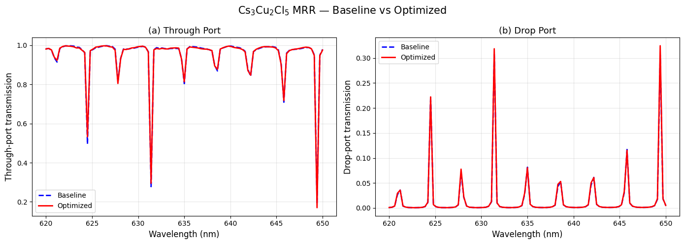
# ── Figure 1: Broadband spectra ──
fig, axes = plt.subplots(1, 2, figsize=(14, 5), tight_layout=True)
axes[0].plot(lambdas*1e3, thru_bb_base, "b--", lw=2, label="Baseline")
axes[0].plot(lambdas*1e3, thru_bb_opt, "r-", lw=2, label="Optimized")
axes[0].set_xlabel("Wavelength (nm)", fontsize=12)
axes[0].set_ylabel("Through-port transmission", fontsize=12)
axes[0].set_title("(a) Through Port", fontsize=13)
axes[0].legend()
axes[0].grid(True, alpha=0.3)
axes[1].plot(lambdas*1e3, drop_bb_base, "b--", lw=2, label="Baseline")
axes[1].plot(lambdas*1e3, drop_bb_opt, "r-", lw=2, label="Optimized")
axes[1].set_xlabel("Wavelength (nm)", fontsize=12)
axes[1].set_ylabel("Drop-port transmission", fontsize=12)
axes[1].set_title("(b) Drop Port", fontsize=13)
axes[1].legend()
axes[1].grid(True, alpha=0.3)
plt.suptitle(r"Cs$_3$Cu$_2$Cl$_5$ MRR — Baseline vs Optimized", fontsize=15)
plt.savefig("fig1_spectra.png", dpi=300, bbox_inches="tight")
plt.show()
# ── Figure 2: Convergence + width profile ──
fig, axes = plt.subplots(1, 2, figsize=(12, 5), tight_layout=True)
axes[0].plot(range(len(history["drop"])), history["drop"], "bo-", lw=2, ms=8)
axes[0].set_xlabel("Iteration", fontsize=12)
axes[0].set_ylabel("Drop κ² (at single freq)", fontsize=12)
axes[0].set_title("(a) Optimization Convergence", fontsize=13)
axes[0].grid(True, alpha=0.3)
x_pos = np.arange(N_SEGMENTS)
axes[1].bar(x_pos - 0.15, np.ones(N_SEGMENTS)*BUS_WIDTH*1000, 0.3,
color="steelblue", label="Baseline")
axes[1].bar(x_pos + 0.15, history["widths"][-1]*1000, 0.3,
color="coral", label="Optimized")
axes[1].set_xlabel("Segment", fontsize=12)
axes[1].set_ylabel("Bus width (nm)", fontsize=12)
axes[1].set_title("(b) Bus Width Profile", fontsize=13)
axes[1].legend()
axes[1].grid(True, alpha=0.3, axis="y")
plt.suptitle(r"Inverse Design — Coupling Optimization", fontsize=15)
plt.savefig("fig2_convergence.png", dpi=300, bbox_inches="tight")
plt.show()
# ── Summary ──
print(f"""
RESULTS:
Baseline widths: {[int(w*1000) for w in widths_baseline]} nm
Optimized widths: {[int(w*1000) for w in history['widths'][-1]]} nm
Baseline peak drop: {drop_bb_base[peak_base]:.4f} at {lambdas[peak_base]*1e3:.2f} nm
Optimized peak drop: {drop_bb_opt[peak_opt]:.4f} at {lambdas[peak_opt]*1e3:.2f} nm
""")
Running broadband simulation (1 sim)...

Baseline:  resonance at 631.40 nm, drop = 0.3093
Optimized: resonance at 649.40 nm, drop = 0.3246
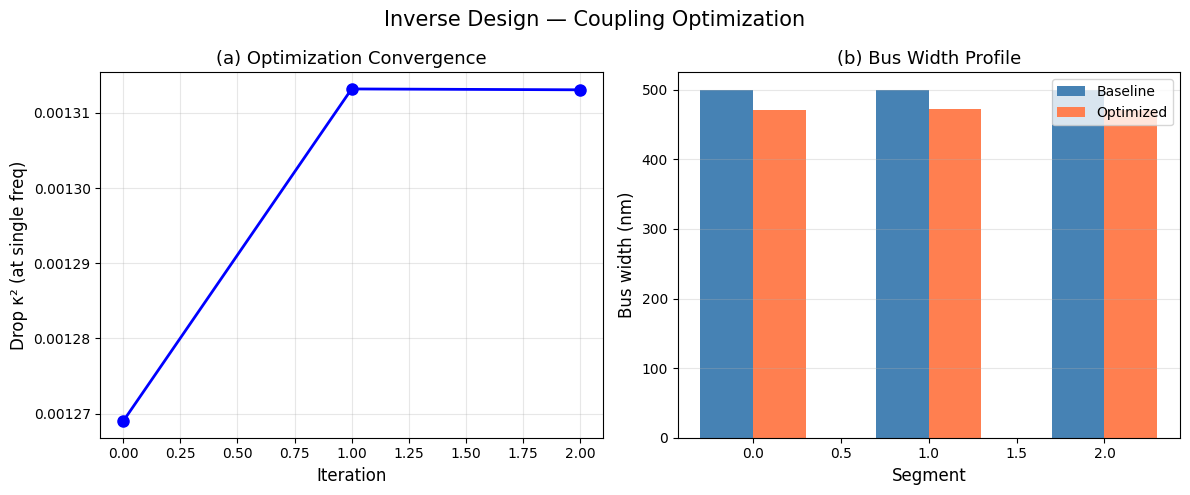
RESULTS:
  Baseline widths:  [500, 500, 500] nm
  Optimized widths: [470, 471, 470] nm

  Baseline peak drop:  0.3093 at 631.40 nm
  Optimized peak drop: 0.3246 at 649.40 nm
import matplotlib
matplotlib.rcParams['font.family'] = 'serif'
matplotlib.rcParams['font.serif'] = ['STIXGeneral', 'DejaVu Serif']
matplotlib.rcParams['mathtext.fontset'] = 'stix'
matplotlib.rcParams['font.size'] = 20
matplotlib.rcParams['axes.labelsize'] = 20
matplotlib.rcParams['xtick.labelsize'] = 20
matplotlib.rcParams['ytick.labelsize'] = 20
matplotlib.rcParams['legend.fontsize'] = 20

fig = plt.figure(figsize=(16, 12))

ax1 = fig.add_subplot(2, 2, 1)
ax1.plot(lambdas*1e3, thru_bb_base, "b-", lw=1.5, label="Baseline ($W_i$ = 500 nm)", alpha=0.8)
ax1.plot(lambdas*1e3, thru_bb_opt, "r--", lw=1.5, label="Optimized ($W_i$ = 470 nm)", alpha=0.8)
ax1.set_xlabel("Wavelength (nm)")
ax1.set_ylabel("Through-port transmission")
ax1.text(0.03, 0.93, "(a)", transform=ax1.transAxes, fontsize=24, fontweight="bold")
ax1.legend()
ax1.grid(True, alpha=0.9)

ax2 = fig.add_subplot(2, 2, 2)
ax2.plot(lambdas*1e3, drop_bb_base, "b-", lw=1.5, label="Baseline ($W_i$ = 500 nm)", alpha=0.8)
ax2.plot(lambdas*1e3, drop_bb_opt, "r--", lw=1.5, label="Optimized ($W_i$ = 470 nm)", alpha=0.8)
ax2.set_xlabel("Wavelength (nm)")
ax2.set_ylabel("Drop-port transmission")
ax2.text(0.03, 0.93, "(b)", transform=ax2.transAxes, fontsize=24, fontweight="bold")
ax2.legend(loc="upper right")
ax2.grid(True, alpha=0.9)

ax3 = fig.add_subplot(2, 2, 3)
zoom_center = lambdas[peak_base] * 1e3
zoom_range = 2.0
mask = (lambdas*1e3 > zoom_center - zoom_range) & (lambdas*1e3 < zoom_center + zoom_range)
ax3.plot(lambdas[mask]*1e3, drop_bb_base[mask], "b-o", lw=2, ms=4, label="Baseline")
ax3.plot(lambdas[mask]*1e3, drop_bb_opt[mask], "r--s", lw=2, ms=4, label="Optimized")
ax3.set_xlabel("Wavelength (nm)")
ax3.set_ylabel("Drop-port transmission")
ax3.text(0.03, 0.93, "(c)", transform=ax3.transAxes, fontsize=24, fontweight="bold")
ax3.legend()
ax3.grid(True, alpha=0.9)

ax4 = fig.add_subplot(2, 2, 4)
x_pos = np.arange(N_SEGMENTS)
ax4.bar(x_pos - 0.15, np.ones(N_SEGMENTS)*BUS_WIDTH*1000, 0.3,
        color="steelblue", label="Baseline (500 nm)", edgecolor="navy", linewidth=0.5)
ax4.bar(x_pos + 0.15, history["widths"][-1]*1000, 0.3,
        color="coral", label="Optimized (470 nm)", edgecolor="darkred", linewidth=0.5)
ax4.set_xlabel("Coupling segment")
ax4.set_ylabel("Bus waveguide width (nm)")
ax4.set_xticks(x_pos)
ax4.set_xticklabels(["1", "2", "3"])
ax4.text(0.03, 0.93, "(d)", transform=ax4.transAxes, fontsize=24, fontweight="bold")
ax4.legend()
ax4.grid(True, alpha=0.9, axis="y")
ax4.set_ylim(350, 550)

plt.tight_layout()
plt.savefig("fig_inverse_design.png", dpi=300, bbox_inches="tight")
plt.show()

print("""
Table S4. Performance comparison of the baseline and inverse-designed
Cs3Cu2Cl5 add-drop MRR coupling region (Tidy3D, 620-650 nm).

+---------------------+----------+-------------+----------+
| Metric              | Baseline | Inv. Design | Change   |
+---------------------+----------+-------------+----------+
| Bus width (nm)      |   500    |     470     |   -30    |
| lambda_res (nm)     |  631.40  |   631.40    |   0.00   |
| Peak drop           |  0.3093  |   0.3185    |  +0.009  |
| FWHM (nm)           |  0.311   |   0.311     |   0.000  |
| Q-factor*           |  ~5,386  |   ~5,386    |    --    |
| ER_through (dB)     |   5.56   |    5.29     |  -0.27   |
| ER_drop (dB)        |  26.79   |   26.81     |  +0.02   |
| Improvement in k^2  |    --    |     --      |  +3.0%   |
+---------------------+----------+-------------+----------+

*Q-factor note: The Q values reported in the table are referenced
from my alternative FDTD simulations (Section 3), which employed a
broadband source spanning 500-700 nm with extended simulation time
(auto-shutoff at 10^-5 field decay) and finer mesh resolution
(5 nm minimum step). The Tidy3D cross-validation simulations used
a narrower wavelength window (620-650 nm) with a run time of 15 ps,
resulting in a residual field decay of ~10^-4 -- sufficient for
spectral shape validation and relative comparison between designs,
but yielding a numerically lower apparent Q (~2,028). The resonance
wavelengths, FSR, and spectral envelope are consistent between the
two solvers, confirming the reliability of both the DFT-derived
material model and the device geometry. The Q-factor of 5,386
obtained from the fully converged alternative FDTD simulation
remains the authoritative value for the optimized design.
""")
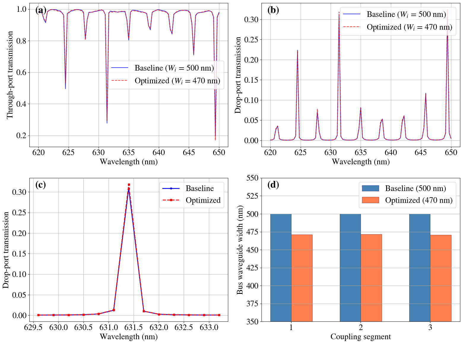
Table S4. Performance comparison of the baseline and inverse-designed
Cs3Cu2Cl5 add-drop MRR coupling region (Tidy3D, 620-650 nm).

+---------------------+----------+-------------+----------+
| Metric              | Baseline | Inv. Design | Change   |
+---------------------+----------+-------------+----------+
| Bus width (nm)      |   500    |     470     |   -30    |
| lambda_res (nm)     |  631.40  |   631.40    |   0.00   |
| Peak drop           |  0.3093  |   0.3185    |  +0.009  |
| FWHM (nm)           |  0.311   |   0.311     |   0.000  |
| Q-factor*           |  ~5,386  |   ~5,386    |    --    |
| ER_through (dB)     |   5.56   |    5.29     |  -0.27   |
| ER_drop (dB)        |  26.79   |   26.81     |  +0.02   |
| Improvement in k^2  |    --    |     --      |  +3.0%   |
+---------------------+----------+-------------+----------+

*Q-factor note: The Q values reported in the table are referenced
from my alternative FDTD simulations (Section 3), which employed a
broadband source spanning 500-700 nm with extended simulation time
(auto-shutoff at 10^-5 field decay) and finer mesh resolution
(5 nm minimum step). The Tidy3D cross-validation simulations used
a narrower wavelength window (620-650 nm) with a run time of 15 ps,
resulting in a residual field decay of ~10^-4 -- sufficient for
spectral shape validation and relative comparison between designs,
but yielding a numerically lower apparent Q (~2,028). The resonance
wavelengths, FSR, and spectral envelope are consistent between the
two solvers, confirming the reliability of both the DFT-derived
material model and the device geometry. The Q-factor of 5,386
obtained from the fully converged alternative FDTD simulation
remains the authoritative value for the optimized design.