Author: William Gorgas, University of Toledo
In this project, we investigate the use of a two-dimensional glass microsphere array as a microlens system to enhance light collection efficiency and improve the signal-to-noise ratio in an on-chip fluorescence microscope. The microspheres act as microlenses that collect and focus emitted fluorescence onto a CMOS sensor, thereby compensating for the lack of traditional imaging optics.
Microlens Use
Microlenses are utilized in fluorescence microscopy to enhance image resolution and light collection efficiency. By focusing and directing excitation light more effectively, microlenses improve the overall fluorescence signal, allowing for better detection of low-abundance targets within a sample. Their importance lies in their ability to increase sensitivity and contrast, making it easier to visualize cellular structures and processes at a microscopic level.
Beyond conventional microscopy, microlenses play a particularly important role in the development of compact and low-cost imaging platforms, such as mobile microscopes. These mobile systems are increasingly vital for point-of-care diagnostics and environmental monitoring, especially in resource-limited settings.
Our implementation
To systematically evaluate and optimize this approach, we employ finite-difference time-domain (FDTD) simulations to model the interaction of emitted fluorescence with the microlens array. In our simulations, fluorophores are approximated as point sources, and their emitted light is propagated through the microspheres to the detector plane. We analyze the optical response across a range of fluorophore-to-microlens distances to understand how this spacing influences light collection, image formation, and signal strength on the sensor.
The fluorophore to microlens distance governs whether the resulting image is virtual or real. By systematically varying these distances in simulation, we establish a theoretical framework to identify the optimal spatial configuration specifically, the relative positioning of the sample, microsphere array, and CMOS sensor, that maximizes signal-to-noise ratio while preserving adequate resolution and field of view.
Overall, this work provides a computational foundation for integrating microlens arrays into on-chip fluorescence imaging systems, with the goal of enabling high-performance, low-cost platforms for biomedical and environmental applications.
FDTD Code
Initialization
The first task was to define the mediums simulated. In this project, this is a simple task as we only account for the vacuum the light travels through, and the Borosilicate glass (n ~ 1.48) that the sphere is made of.
import tidy3d as td
import numpy as np
import tidy3d.plugins.design as tdd
import matplotlib.pyplot as plt
from scipy.ndimage import gaussian_filter1d

vacuum = td.Medium(
    name = 'Vacuum'
)

glass = td.Medium(
    name = 'glass',
    permittivity = 2.1904 # n = 1.48
)

sphere_radius = 75  # microns
2. Define Pre- and Post-Processing Functions
The Design plugin works by splitting the simulation workflow into:
-
pre: takes parameter values, returns atd.Simulation -
post: takestd.SimulationData, returns a dict of results
The plugin then handles batching all simulations and running them in parallel on the Tidy3D cloud.
We start the definition by grouping together the point source and the microsphere. The distance between the two is the main relationship we are exploring.
We define sim_x as the total simulation size in the x-direction. This size is influenced by how long the distance from the source to the sphere is, plus an arbitrary distance ("visualization constant") following the sphere that is big enough to analyze the image formation properly. In this example, 300 microns was used. In the y and z directions, a buffer of +3 is used to avoid Structure-PML interaction.
We chose to highlight a range of distances outside of the focal length, as those produce global maxima outside (>75μm) the center of the microsphere. The equation for the effective focal length (EFL) of a ball lens is given by: $$ f = \frac{nR}{2(n - 1)} $$ and, for n = 1.48 & R = 75μm, yields EFL ~= 116μm (BFL ~= 41μm). Therefore, we choose source distances 130μm, 140μm, 200μm, 300μm, 400μm, & 500μm to get an adequate picture of the correlation.
def pre(distance: int) -> td.Simulation:
    """Create a Tidy3D simulation for a given fluorophore-to-sphere distance.

    The visualization constant is derived from the distance to ensure
    adequate space for analyzing image formation beyond the sphere.
    """
    constant = max(300, distance + 160)

    pointdipole = td.PointDipole(
        name="pointdipole_0",
        center=[-distance, 0, 0],
        source_time=td.GaussianPulse(freq0=193615962458333.3, fwidth=6245676208333.328),
        polarization="Ey",
    )

    sphere = td.Structure(
        geometry=td.Sphere(radius=sphere_radius, center=[0, 0, 0]),
        name="sphere_0",
        medium=glass,
    )

    sim_x = distance + sphere_radius + constant
    sim_center = -distance + (sim_x / 2)

    field_monitor = td.FieldMonitor(
        name="field",
        size=[sim_x, 0, 153],
        center=[sim_center, 0, 0],
        freqs=td.C_0 / 1.55,
    )

    dl_fine = 0.155
    dl_coarse = 0.31

    # Fine mesh around the sphere to properly resolve the dielectric interface.
    # Covers a 190x160x160 box centered on the sphere (sphere_radius + 20 µm buffer).
    sphere_fine_mesh = td.MeshOverrideStructure(
        geometry=td.Box(center=[0, 0, 0], size=[190, 160, 160]),
        dl=(dl_fine, dl_fine, dl_fine),
        name="sphere_fine_mesh",
    )

    # Coarser mesh for the far observation region beyond the sphere.
    # This region is large (hundreds of µm) but contains only smoothly
    # varying vacuum fields, so 2x coarser spacing is adequate.
    far_x_start = 95.0
    far_x_end = sphere_radius + constant + 1
    far_coarse_mesh = td.MeshOverrideStructure(
        geometry=td.Box(
            center=[(far_x_start + far_x_end) / 2, 0, 0],
            size=[far_x_end - far_x_start, td.inf, td.inf],
        ),
        dl=(dl_coarse, dl_coarse, dl_coarse),
        enforce=True,
        name="far_coarse_mesh",
    )

    sim = td.Simulation(
        size=[sim_x + 1, 153, 153],
        center=[sim_center, 0, 0],
        grid_spec=td.GridSpec.auto(
            wavelength=1.55,
            min_steps_per_wvl=10,
            override_structures=[sphere_fine_mesh, far_coarse_mesh],
        ),
        run_time={"quality_factor": 1, "source_factor": 3},
        medium=vacuum,
        sources=[pointdipole],
        monitors=[field_monitor],
        structures=[sphere],
    )

    return sim
Photon Density Calculation
Setup
The key relationship to find photon density from |E| is the electromagnetic energy density of a wave in a medium:
$$u = \frac{\varepsilon}{2} |E|^2$$
where $\varepsilon = n^2 \varepsilon_0$ is the permittivity of the medium and $E$ is the electric field amplitude. This tells us how much energy per unit volume is stored in the field at any point in space.
To convert this energy density into a photon number density, we divide by the energy of a single photon:
$$E_{\text{photon}} = \frac{hc}{\lambda}$$
So the photon density is:
$$\rho_{\text{photon}} = \frac{u}{E_{\text{photon}}} = \frac{\varepsilon |E|^2}{2 h c / \lambda}$$
Geometry / Dielectric
The sphere has refractive index $n = 1.48$, so the permittivity inside of it is:
$$\varepsilon = n^2 \varepsilon_0$$
We define the sphere geometry and build a boolean mask that we will later use to apply the correct permittivity at every grid point.
e_0 = 8.854e-12
h_planck = 6.626e-34
c_light = 3e8
wavelength = 1.55e-6
photon_energy = h_planck * c_light / wavelength

n_dielectric = 1.48
Loading FDTD Data
The FDTD solver outputs the field at every grid point as a flat table: each row is (x, y, E_value). We need to reshape this into a proper 2D array so that value[i, j] gives the field at position (x[i], y[j]).
The solver exports the magnitude $|E|$ at each point, not the field directly. The relevant quantity for energy is $|E|^2$ (intensity), so we must square it.
Photon Density vs distance
We collapse the transverse ($y$) dimension by taking the mean across each $x$-slice — a discrete approximation to integrating over the beam cross-section:
$$\langle\rho\rangle(x) = \frac{1}{L_y}\int \rho(x,y)\,dy$$
This gives the average photon density at each x value.
Additionally, we only track values above x = 75 to ensure we find the location of the maxima on the side on which the image is formed, and NOT the maximum where the point source is located, for instance.
Both (3 & 4) of these tasks are done through a single function to streamline processing of multiple datasets
def post(data: td.SimulationData) -> dict:
    """Process the simulation data to find the location and value of max photon density.

    Computes the E-field magnitude, converts to photon density,
    and finds the x-position of the peak density beyond the sphere.
    """
    field_data = data["field"]

    Ex = np.abs(field_data.Ex.values)
    Ey = np.abs(field_data.Ey.values)
    Ez = np.abs(field_data.Ez.values)
    magnitude = np.sqrt(Ex**2 + Ey**2 + Ez**2)

    magnitude = np.squeeze(magnitude)
    intensity = magnitude**2

    x = field_data.Ex.x.values
    z = field_data.Ex.z.values

    xx, zz = np.meshgrid(x, z, indexing="ij")
    inside_sphere = xx**2 + zz**2 <= sphere_radius**2
    intensity_corrected = np.where(inside_sphere, intensity * n_dielectric, intensity)

    photon_density = (e_0 / 2) * intensity_corrected / photon_energy

    x_mask = x > sphere_radius
    photon_density_masked = photon_density.copy()
    photon_density_masked[~x_mask, :] = -np.inf

    profile = np.mean(photon_density_masked[x_mask, :], axis=1)
    max_idx = np.argmax(profile)
    max_x = float(x[x_mask][max_idx])
    max_profile_value = float(profile[max_idx])

    return {
        "max_density_x": max_x,
        "max_density_value": max_profile_value,
    }
Verify a Sample Simulation
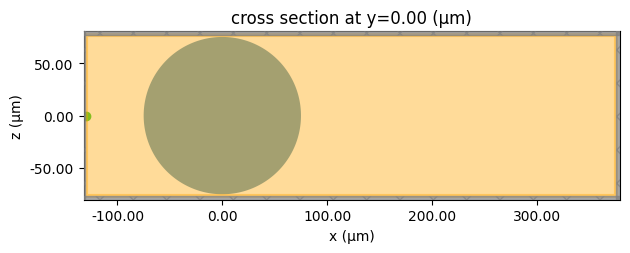
pre(130).plot(y=0)
<Axes: title={'center': 'cross section at y=0.00 (μm)'}, xlabel='x (μm)', ylabel='z (μm)'>
Run the Design Space Exploration
The Design plugin will:
- Call
pre(distance)for each distance value - Batch all simulations together for parallel execution on the cloud
- Call
post(sim_data)for each result - Store everything in a
Resultobject
distances = [130, 140, 200, 300, 400, 500]

param_distance = tdd.ParameterAny(name="distance", allowed_values=distances)

method = tdd.MethodGrid()

design_space = tdd.DesignSpace(
    parameters=[param_distance],
    method=method,
    task_name="Microlens_Design",
    path_dir="./data",
)
results = design_space.run(pre, post)
10:13:38 EDT Running 6 Simulations
10:14:40 EDT WARNING: Simulation final field decay value of 0.000144 is greater
             than the simulation shutoff threshold of 1e-05. Consider running
             the simulation again with a larger 'run_time' duration for more
             accurate results.
10:14:41 EDT WARNING: Simulation final field decay value of 5.95e-05 is greater
             than the simulation shutoff threshold of 1e-05. Consider running
             the simulation again with a larger 'run_time' duration for more
             accurate results.
             WARNING: Simulation final field decay value of 2.03e-05 is greater
             than the simulation shutoff threshold of 1e-05. Consider running
             the simulation again with a larger 'run_time' duration for more
             accurate results.
10:14:42 EDT WARNING: Simulation final field decay value of 1.26e-05 is greater
             than the simulation shutoff threshold of 1e-05. Consider running
             the simulation again with a larger 'run_time' duration for more
             accurate results.
             WARNING: Simulation final field decay value of 1.1e-05 is greater
             than the simulation shutoff threshold of 1e-05. Consider running
             the simulation again with a larger 'run_time' duration for more
             accurate results.
df = results.to_dataframe()
df
| distance | max_density_x | max_density_value | |
|---|---|---|---|
| 0 | 130 | 290.250000 | 258013600.0 |
| 1 | 140 | 252.430000 | 259395744.0 |
| 2 | 200 | 165.561983 | 204321600.0 |
| 3 | 300 | 130.330000 | 123189744.0 |
| 4 | 400 | 118.149053 | 79960096.0 |
| 5 | 500 | 111.470000 | 55442156.0 |
Plotting / Visualization
Photon Density vs Distance from Sphere Center
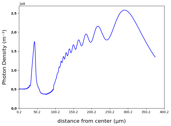
As an example, we can visualize the photon density profile for the 130 µm source distance case. The x-axis will represent the distance from the center of the sphere, and the y-axis will represent the photon density
Similar to get_max_photon_density_location, this visualization only takes values above x = 0 (sphere center) into consideration.
sim_data_130 = td.SimulationData.from_file(results.task_paths[0])

field_data = sim_data_130["field"]
Ex = np.abs(field_data.Ex.values)
Ey = np.abs(field_data.Ey.values)
Ez = np.abs(field_data.Ez.values)
magnitude = np.sqrt(Ex**2 + Ey**2 + Ez**2)

magnitude = np.squeeze(magnitude)
intensity = magnitude**2

x = field_data.Ex.x.values
z = field_data.Ex.z.values

xx, zz = np.meshgrid(x, z, indexing="ij")
inside_sphere = xx**2 + zz**2 <= sphere_radius**2
intensity_corrected = np.where(inside_sphere, intensity * n_dielectric, intensity)
photon_density_130 = (e_0 / 2) * intensity_corrected / photon_energy

x_mask = x > 0
x_plot = x[x_mask]
y_plot = gaussian_filter1d(np.mean(photon_density_130[x_mask, :], axis=1), sigma=1)

fig, ax = plt.subplots(figsize=(8, 6))
ax.plot(x_plot, y_plot, color="blue")
ax.set_xlabel("distance from center (\u00b5m)", fontsize=16, labelpad=16)
ax.set_ylabel("Photon Density (m\u207b\u00b3)", fontsize=16, labelpad=12)

xticks = np.arange(x_plot[0], x_plot[-1] + 50, 50)
ax.set_xticks(xticks)
for label in ax.get_yticklabels():
    label.set_fontweight("bold")
ax.set_xlim(left=x_plot[0])
ax.set_ylim(bottom=0)
ax.tick_params(axis="y", labelsize=10)
plt.subplots_adjust(bottom=0.15)
plt.show()
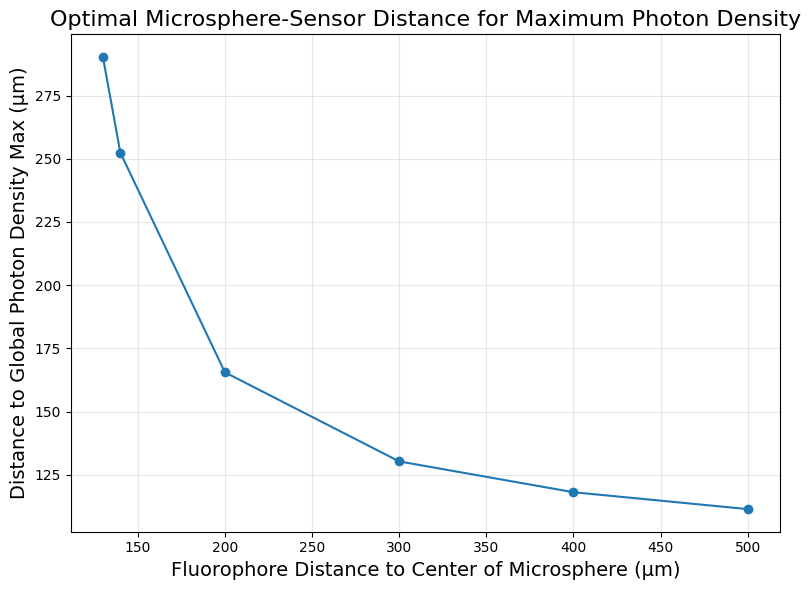
Final Graph
As previously mentioned, the main metric we're after is
Distance to Global Density Maximum vs Source Distance
where both distances are measured from the center of the microsphere. We can get this data by utilizing the previously defined function for all of our datasets
For this set of fluorophore distances, we can see a clear inverse correlation between the two variables.
fig, ax = plt.subplots(figsize=(8, 6))

ax.plot(df["distance"], df["max_density_x"], marker="o", color="tab:blue")
ax.set_xlabel("Fluorophore Distance to Center of Microsphere (\u00b5m)", fontsize=14)
ax.set_ylabel("Distance to Global Photon Density Max (\u00b5m)", fontsize=14)
ax.set_title("Optimal Microsphere-Sensor Distance for Maximum Photon Density", fontsize=16)
ax.grid(True, alpha=0.3)

plt.tight_layout()
plt.show()