author: Dun Wang, University of Pennsylvania

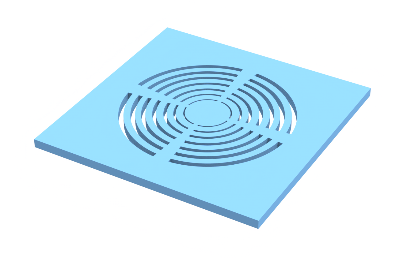
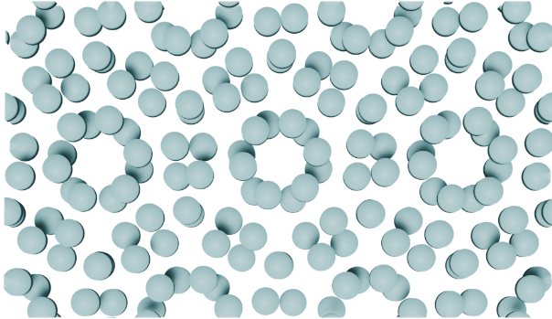
Twisted bilayer photonic crystal (TBPC) structures have attracted significant attention due to their unique resonance properties and strong connection to phenomena observed in 2D materials. The twist angle introduces new coupling effects and Moiré patterns, leading to rich optical responses. Studying their reflection spectrum provides insight into these resonances and their potential applications in photonics.

diagram

[1]:

import numpy as np
import matplotlib.pyplot as plt

import tidy3d as td
import tidy3d.web as web

Define Study Parameters¶

We now define global parameters for the simulation.

[2]:

rng = np.random.default_rng(12345)

# period
a = 0.5

# thickness of each slab
H = 0.2

# diameter of the air holes, at A or B sublattice
d_A = 0.2
d_B = 0.2

# space between the slabs and PMLs
h_space = 2

# inter-layer spacing
h_layer = 0.13

# alpha: twist angle for commensurate Moiré pattern (I,I+1) rot_angle: rotate the moire lattice vectors in alignment with xy axis
I = 1
rot_angle = np.arccos((1.5 * I + 0.5) / np.sqrt(3 * I**2 + 3 * I + 1)) - np.pi / 6
alpha = np.arccos(
    (3 * I**2 + 3 * I + 0.5) / (3 * I**2 + 3 * I + 1)
)  # I=1 corresponds to the largest commensurate angle 21.79 degrees

# dt= strength of Wu-Hu perturbation
dt = 0.015

# light incident angle
theta = 0
phi = 0

freqs = np.linspace(2e14, 3.5e14, 2000)  # frequency range
freq0 = (freqs[0] + freqs[-1]) / 2
wl0 = td.C_0 / freq0
fwidth = np.abs(freqs[0] - freqs[-1])
pulse_width = fwidth
run_time = 600 / pulse_width

n_air = 1
n_medium = 2.02
n_bg = 1.46
SiN = td.Medium(permittivity=n_medium**2)
SiO2 = td.Medium(permittivity=n_bg**2)
Air = td.Medium(permittivity=n_air**2)

N = 30  # max number of unit cells allowed
# Simulation size is set as one moire unit cell after perturbation
sim_size = (
    np.sqrt(3 * I**2 + 3 * I + 1) * np.sqrt(3) * a,
    np.sqrt(3) * np.sqrt(3 * I**2 + 3 * I + 1) * np.sqrt(3) * a,
    2 * h_space + 2 * H + h_layer,
)

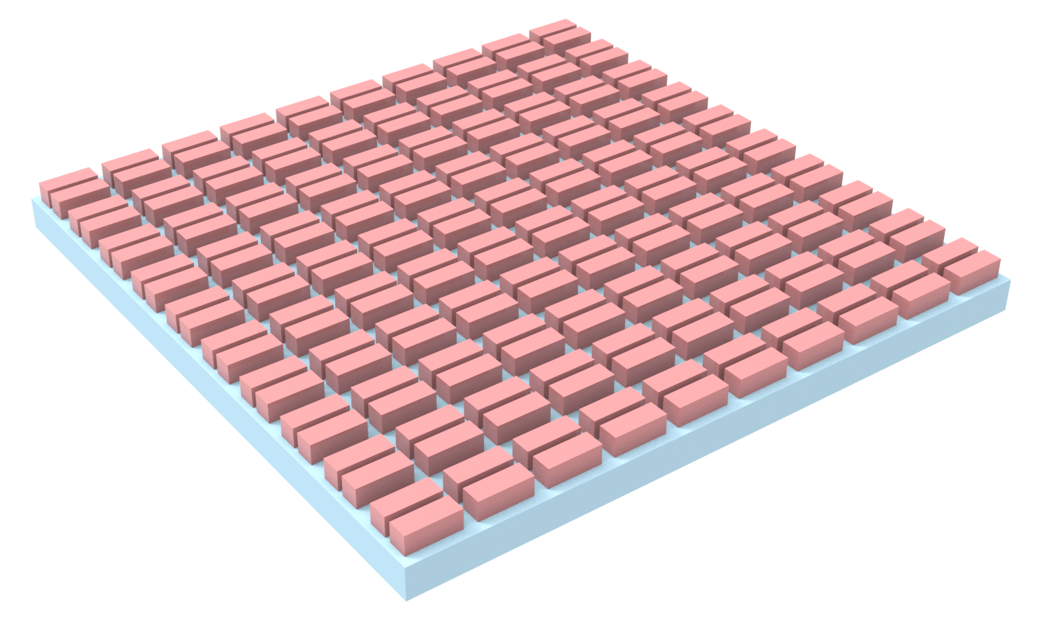
Define Geometry¶

The geometry consists of etched holes twisted in two SiN layers, separated by air. For defining the rotated holes, we define an auxiliary function.

[3]:

# first SiN slab (bottom layer)
slab1 = td.Structure(
    geometry=td.Box(
        center=(0, 0, 0),
        size=(td.inf, td.inf, H),
    ),
    medium=SiN,
    name="slab1",
)


# air spacer between slabs
spacer = td.Structure(
    geometry=td.Box(
        center=(0, 0, H / 2 + h_layer / 2),
        size=(td.inf, td.inf, h_layer),
    ),
    medium=Air,
    name="spacer",
)

# second SiN slab (top layer)
slab2 = td.Structure(
    geometry=td.Box(
        center=(0, 0, H + h_layer),
        size=(td.inf, td.inf, H),
    ),
    medium=SiN,
    name="slab2",
)

# air substrate/superstrate
sub = td.Structure(
    geometry=td.Box(
        center=(0, 0, -h_space - H / 2),
        size=(td.inf, td.inf, h_space * 2),
    ),
    medium=Air,
    name="sub",
)


layers = [sub, slab1, spacer, slab2]


# Add holes in one layer with angle theta w.r.t x axis, at height h, lateral shift shift, Wu-Hu perturbation dt
def hex_holes(a, d_A, d_B, theta, h, shift, dt):
    holes = []
    A1 = np.array(
        [
            3 * a / 2 * np.cos(theta) - np.sqrt(3) * a / 2 * np.sin(theta),
            3 * a / 2 * np.sin(theta) + np.sqrt(3) * a / 2 * np.cos(theta),
            0,
        ]
    )
    A2 = np.array(
        [
            3 * a / 2 * np.cos(theta) + np.sqrt(3) * a / 2 * np.sin(theta),
            3 * a / 2 * np.sin(theta) - np.sqrt(3) * a / 2 * np.cos(theta),
            0,
        ]
    )
    Rot = np.array(
        [
            [np.cos(theta), -np.sin(theta), 0],
            [np.sin(theta), np.cos(theta), 0],
            [0, 0, 1],
        ]
    )
    t1 = Rot @ np.array([0, -a / np.sqrt(3) + dt, 0])
    t2 = Rot @ np.array(
        [-(a / np.sqrt(3) - dt) * np.sqrt(3) / 2, -(a / np.sqrt(3) - dt) / 2, 0]
    )
    t3 = Rot @ np.array(
        [-(a / np.sqrt(3) - dt) * np.sqrt(3) / 2, (a / np.sqrt(3) - dt) / 2, 0]
    )
    t4 = Rot @ np.array([0, a / np.sqrt(3) - dt, 0])
    t5 = Rot @ np.array(
        [(a / np.sqrt(3) - dt) * np.sqrt(3) / 2, (a / np.sqrt(3) - dt) / 2, 0]
    )
    t6 = Rot @ np.array(
        [(a / np.sqrt(3) - dt) * np.sqrt(3) / 2, -(a / np.sqrt(3) - dt) / 2, 0]
    )

    for i in np.arange(-N, N + 1, 1):
        for j in np.arange(-N, N + 1, 1):
            r1 = np.array([0, shift, h]) + i * A1 + j * A2 + t1
            tol = 0.1
            if (np.abs(r1[0]) <= np.min([N * a, sim_size[0] / 2 + tol])) & (
                np.abs(r1[1]) <= np.min([N * a, sim_size[1] / 2 + tol])
            ):
                holes.append(
                    td.Structure(
                        geometry=td.Cylinder(
                            radius=d_A / 2, center=tuple(r1), length=H, axis=2
                        ),
                        medium=Air,
                    )
                )
            r2 = np.array([0, shift, h]) + i * A1 + j * A2 + t2
            if (np.abs(r2[0]) <= np.min([N * a, sim_size[0] / 2 + tol])) & (
                np.abs(r2[1]) <= np.min([N * a, sim_size[1] / 2 + tol])
            ):
                holes.append(
                    td.Structure(
                        geometry=td.Cylinder(
                            radius=d_B / 2, center=tuple(r2), length=H, axis=2
                        ),
                        medium=Air,
                    )
                )
            r3 = np.array([0, shift, h]) + i * A1 + j * A2 + t3
            if (np.abs(r3[0]) <= np.min([N * a, sim_size[0] / 2 + tol])) & (
                np.abs(r3[1]) <= np.min([N * a, sim_size[1] / 2 + tol])
            ):
                holes.append(
                    td.Structure(
                        geometry=td.Cylinder(
                            radius=d_A / 2, center=tuple(r3), length=H, axis=2
                        ),
                        medium=Air,
                    )
                )
            r4 = np.array([0, shift, h]) + i * A1 + j * A2 + t4
            if (np.abs(r4[0]) <= np.min([N * a, sim_size[0] / 2 + tol])) & (
                np.abs(r4[1]) <= np.min([N * a, sim_size[1] / 2 + tol])
            ):
                holes.append(
                    td.Structure(
                        geometry=td.Cylinder(
                            radius=d_B / 2, center=tuple(r4), length=H, axis=2
                        ),
                        medium=Air,
                    )
                )
            r5 = np.array([0, shift, h]) + i * A1 + j * A2 + t5
            if (np.abs(r5[0]) <= np.min([N * a, sim_size[0] / 2 + tol])) & (
                np.abs(r5[1]) <= np.min([N * a, sim_size[1] / 2 + tol])
            ):
                holes.append(
                    td.Structure(
                        geometry=td.Cylinder(
                            radius=d_A / 2, center=tuple(r5), length=H, axis=2
                        ),
                        medium=Air,
                    )
                )
            r6 = np.array([0, shift, h]) + i * A1 + j * A2 + t6
            if (np.abs(r6[0]) <= np.min([N * a, sim_size[0] / 2 + 0.1])) & (
                np.abs(r6[1]) <= np.min([N * a, sim_size[1] / 2 + 0.1])
            ):
                holes.append(
                    td.Structure(
                        geometry=td.Cylinder(
                            radius=d_B / 2, center=tuple(r6), length=H, axis=2
                        ),
                        medium=Air,
                    )
                )

    return holes

Define Sources, Monitors, and the Simulation Object¶

The source is a circularly polarized source, defined by two plane waves with orthogonal polarizations and a π/2 phase difference.

We will also place FluxMonitors to record transmitted and reflected fields, and FieldMonitors for visualization.

Finally, we define a makesim function to generate the model as a function of the source’s incident angle.

[4]:

def circular_source(pol, theta, phi):
    # define a circularly polarized plane wave incident at angle theta phi
    plane_wave_x = td.PlaneWave(
        source_time=td.GaussianPulse(freq0=freq0, fwidth=pulse_width),
        size=(td.inf, td.inf, 0),
        center=(0, 0, 1.5 * H + h_layer + 0.5 * h_space),
        direction="-",
        angle_theta=theta,
        angle_phi=phi,
        pol_angle=0,
    )

    # determine the phase difference given the polarization
    if pol == "LCP":
        phase = -np.pi / 2
    elif pol == "RCP":
        phase = np.pi / 2
    else:
        raise ValueError("pol must be `LCP` or `RCP`")

    # define a plane wave polarized in the y direction with a phase difference
    plane_wave_y = td.PlaneWave(
        source_time=td.GaussianPulse(freq0=freq0, fwidth=pulse_width, phase=phase),
        size=(td.inf, td.inf, 0),
        center=(0, 0, 1.5 * H + h_layer + 0.5 * h_space),
        direction="-",
        angle_theta=theta,
        angle_phi=phi,
        pol_angle=np.pi / 2,
    )

    return [plane_wave_x, plane_wave_y]


# In this simulation we only use the reflection monitor monitor_r. The others can be used to record the field distributions.
monitor_r = td.FluxMonitor(
    center=[0, 0, 1.5 * H + h_layer + 0.9 * h_space],
    size=[td.inf, td.inf, 0],
    freqs=freqs,
    name="R",
)
monitor_t = td.FluxMonitor(
    center=[0, 0, -0.5 * H - 0.9 * h_space],
    size=[td.inf, td.inf, 0],
    freqs=freqs,
    name="T",
)
monitor_fz = td.FieldMonitor(
    center=[0, 0, H / 2 + h_layer / 2], size=[td.inf, td.inf, 0], freqs=freqs, name="Fz"
)
monitor_fx = td.FieldMonitor(
    center=[0, 0, 0], size=[0, td.inf, td.inf], freqs=freqs, name="Fx"
)


# Make the simulation. j is a label used in the batch
def makesim(pol: str, theta: float, phi: float, dt: float, j: int):
    source = circular_source(pol, theta, phi)
    structures = (
        layers
        + hex_holes(a, d_A, d_B, -rot_angle, 0, 0, 0)
        + hex_holes(a, d_A, d_B, -rot_angle + alpha, H + h_layer, 0, dt)
    )

    # Bloch boundaries from source.
    bloch_x = td.Boundary.bloch_from_source(
        source=source[0], domain_size=sim_size[0], axis=0, medium=Air
    )

    bloch_y = td.Boundary.bloch_from_source(
        source=source[0], domain_size=sim_size[1], axis=1, medium=Air
    )

    bspecs = td.BoundarySpec(x=bloch_x, y=bloch_y, z=td.Boundary.pml())

    sim = td.Simulation(
        size=sim_size,
        center=(0, 0, H / 2 + h_layer / 2),
        grid_spec=td.GridSpec.auto(min_steps_per_wvl=8, wavelength=wl0),
        structures=structures,
        medium=Air,
        sources=source,
        monitors=[monitor_r],
        run_time=run_time,
        boundary_spec=bspecs,
        shutoff=1e-5,
    )
    return sim

Make a Batch of Simulations With Different Incident Angles¶

Now, we create a Batch of simulations with different incident angles to run them all in parallel.

[5]:

sims = {}
angle_max = 25 * np.pi / 180
N_angle = 100

# High symmetry points in K space are defined for convenience
a_M = sim_size[1]
K_plus = np.array([1 / (np.sqrt(3) * a_M), 1 / (3 * a_M)])
K_minus = np.array([1 / (np.sqrt(3) * a_M), -1 / (3 * a_M)])
K_up = np.array([0, 2 / (3 * a_M)])
K_down = np.array([0, -2 / (3 * a_M)])
M_plus = np.array([1 / (np.sqrt(3) * a_M), 0])
M_minus = np.array([-1 / (np.sqrt(3) * a_M), 0])
Gamma = np.array([0, 0])
k_start = Gamma
k_end = (
    1 / wl0 * np.sin(angle_max)
)  # k_end can be set either as one special point in K space or with a maximum incident angle angle_max

# The angular scan proceeds with a fixed step size in wavevector k
for i in range(N_angle):
    k_i = k_start + i / N_angle * (k_end - k_start)
    if np.linalg.norm(k_i) != 0:
        theta = np.arcsin(np.linalg.norm(k_i) * wl0)
        phi = np.arcsin(k_i[1] / np.linalg.norm(k_i)) + np.pi * (k_i[0] < 0)
    else:
        theta = 0
        phi = 0
    sims[f"sim_{i}"] = makesim("RCP", theta, phi, dt, i)

# Create the Batch object
batch = web.Batch(simulations=sims, folder_name="data", verbose=True)

We can now plot one simulation to inspect the setup.

[6]:

# Visualize the first simulation
sims["sim_0"].plot_3d()
plt.show()

[7]:

# estimate the maximum cost for the whole Batch
_ = batch.estimate_cost()

10:08:57 -03 Maximum FlexCredit cost: 4.821 for the whole batch.

Run the Batch of Simulations¶

[8]:

batch_data = batch.run(path_dir="data")

Output()

10:10:02 -03 Started working on Batch containing 100 tasks.

10:13:03 -03 Maximum FlexCredit cost: 4.821 for the whole batch.

             Use 'Batch.real_cost()' to get the billed FlexCredit cost after the
             Batch has completed.

Output()

10:18:52 -03 Batch complete.

Output()

Postprocessing¶

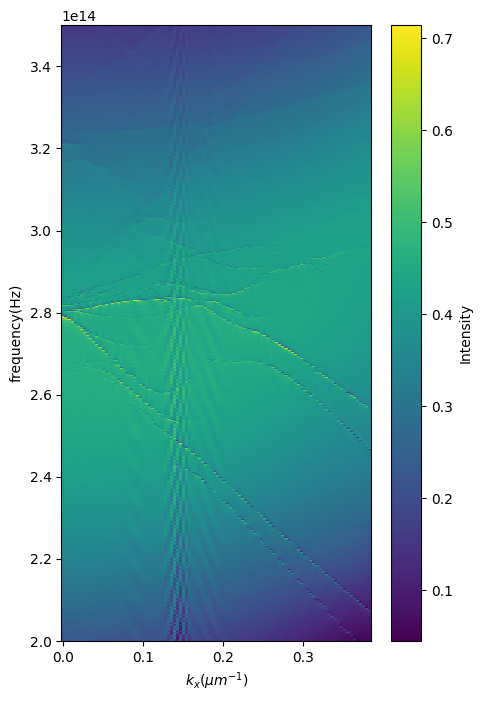
Finally, we can analyze the reflection of the bilayer as a function of the incident angle.

Since we are dealing with resonant structures, the fields do not always fully decay by the end of the simulation. For this reason, we add the following line to suppress the related warning messages.

[9]:

td.config.logging_level = "ERROR"

[10]:

# Collect all reflection data in flux_sig
flux_sig = np.zeros((0, len(freqs)))
for i in range(N_angle):
    flux_sig = np.vstack(
        (flux_sig, batch_data[f"sim_{i}"].monitor_data["R"].flux.squeeze())
    )


# plot the angle-resolved reflection spectrum
angle_max = np.arcsin(k_end * wl0)  # enter the proper maximum angle
K, F = np.meshgrid(k_end * np.arange(N_angle) / N_angle, freqs)
flux_plot = flux_sig / 2


plt.figure(figsize=(5, 8))
plt.pcolormesh(K.T, F.T, flux_plot, shading="nearest", cmap="viridis")
plt.colorbar(label="Intensity")

plt.rcParams["text.usetex"] = True
plt.xlabel("$k_x (\mu m^{-1})$")
plt.ylabel("frequency(Hz)")


plt.show()