Tidy3D provides two methods for simulating angled plane waves for periodic structures:
Fixed in-plane k vector mode, and
Fixed angle mode.
Both methods produce the same results at the central source frequency, but their behavior away from the central frequency differs significantly and it is important to understand the differences between the two approaches.
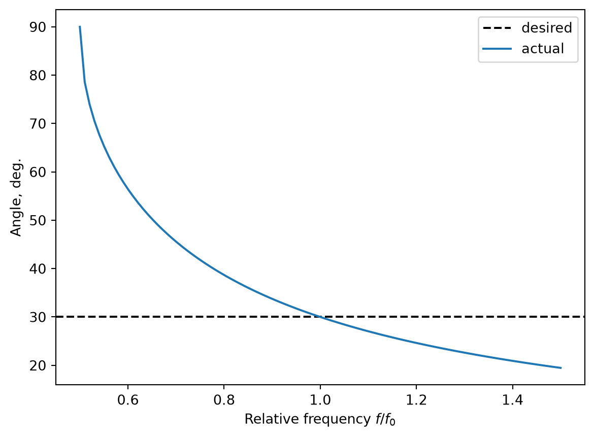
The first method is based on injecting an angled plane wave source and imposing the Bloch boundary conditions on periodic domain edges (see tutorial on boundary conditions for details). Fields that satisfy Bloch boundary conditions undergo a change of constant factor across periodic boundaries. For example, if a plane wave with frequency \(f_0\) and angle \(\theta_0\) with the \(x\) axis is propagating along axis \(z\), then the fields will differ by a factor of \(\exp(-i \sin(\theta_0) f_0 L_x)\) between opposite edges in the \(x\) direction. If we consider another plane wave with the same angle but a different frequency \(f_1\), then this second plane wave would undergo a different phase difference of \(\exp(-i \sin(\theta_0) f_1 L_x)\). However, the FDTD method performs evolution of time domain fields, which consist of a continuous spectrum of waves in a certain frequency range, and only single phase factor can be applied at periodic Bloch boundaries. Typically, this factor is selected to correspond to the central frequency of the injected plane wave, which means that only fields at the central frequency would satisfy the desired angle. Angles of frequency domain fields computed for wavelengths away from the central one will differ from \(\theta_0\). By performing simple calculations it is easy to show that the field angle dependence on frequency is \(\theta_{actual}(f) = \arcsin(\sin(\theta_0) \frac{f_0}{f})\).
A simple code below visualizes this dependence in case of \(\theta_0 = 30\) deg.
The second approach avoids the issue of angular frequency dependency by modifying the governing Maxwell equations to include the correct phase difference for all frequencies. The resulting equations to be solved in fact represent propagation of normally incident plane wave but with additional coupling factors. These coupling terms increase the computational complexity, which leads to the following two disadvantages of the second approach compared to the first one.
1. Simulation cost
First of all, it increases the cost of running a simulation: the fixed angle technique could lead to a significant increase of simulation cost. This increase depends on the angle of propagation plane wave. For example, for a plane wave inclined at angle \(\theta=5\) degrees the simulation cost increase compared to the fixed in-plane k simulation would be approximately a factor of 2, while for a plane wave angled at \(\theta = 50\) degrees such an increase would be approximately a factor of 4. The user is encouraged to use web.estimate() cost estimation function before submitting simulation for running.
Despite increased simulation costs, the fixed angle technique can significantly outperform the fixed in plane k technique if many frequency points are of interest. For example, to accurately compute scattering and transmission of an oblique plane wave at a given angle of \(\theta = 50\) deg. and at 100 frequency points using Bloch BC it would require creating a parameter sweep of the source central frequency. Essentially treating each simulation as a frequency domain simulation. Since tasks are run in parallel on Flexcompute servers, the speed might not actually be much worse but the cost linearly scales with the number of sampled frequency points. While using the fixed angle technique it would require only one simulation resulting, with the total cost reduced by a factor of [cost of running 100 Bloch BC simulations] / [cost of running 1 fixed angle simulation] = 100 / 4 = 25.
2. Stability
Another disadvantage of the fixed angle technique that couple from additional coupling terms, is more frequent divergence issues. In most cases this could be alleviated by either reducing the courant factor or switching absorbing boundary conditions in the propagation direction to adiabatic Absorber. Overall, the user should exercise more caution when dealing with fixed angle simulations.
Tidy3D Python API
Oblique incident plane waves can be defined in Tidy3D Python API using source types TFSF and PlaneWave. Currently, TFSF supports only the fixed in-plane k approach, while PlaneWave supports both. Switching between the two techniques for PlaneWave sources is simply accomplished by changing the field angular_spec from FixedInPlaneKSpec (default) to FixedAngleSpec. Additionally, for the fixed in plane k simulations Bloch boundary conditions must be correctly set up, while for the fixed angle simulations periodic boundary conditions are simply set to Periodic.
Demonstration: Transmission through a Dispersive Stack.
# Wavelength and frequency rangelambda_range = (0.5, 1.5)lam0 = np.sum(lambda_range) /2freq_range = (td.constants.C_0 / lambda_range[1], td.constants.C_0 / lambda_range[0])Nfreq =333# frequencies and wavelengths of monitormonitor_freqs = np.linspace(freq_range[0], freq_range[1], Nfreq)monitor_lambdas = td.constants.C_0 / monitor_freqs# central frequency, frequency pulse width and total running timefreq0 = monitor_freqs[Nfreq //2]freqw =0.3* (freq_range[1] - freq_range[0])
We will consider a stack of 4 layers with thicknesses 0.5, 0.2, 0.4, and 0.3 \(\mu m\).
# Thicknesses of slabst_slabs = [0.5, 0.2, 0.4, 0.3] # um# space between slabs and sources and PMLspacing =1* lambda_range[-1]# simulation sizesim_size = Lx, Ly, Lz = (0.2, 1, 4* spacing +sum(t_slabs))
Layers are made or dispersive and non-dispersive materials.
# Materials# simple dielectric, background materialmat0 = td.Medium(permittivity=1)# simple, lossy materialmat1 = td.Medium(permittivity=4.0, conductivity=0.01)# active material with n & k values at a specified frequency or wavelengthmat2 = td.Medium.from_nk(n=3.0, k=0.1, freq=freq0)# weakly dispersive material defined by dn_dwvl at a given frequencymat3 = td.Sellmeier.from_dispersion(n=2.0, dn_dwvl=-0.1, freq=freq0)# dispersive material from tidy3d librarymat4 = td.material_library["BK7"]["Zemax"]# put all togethermat_slabs = [mat1, mat2, mat3, mat4]
Given the defined layer thicknesses and material definition, programmatically create corresponding Tidy3D structures.
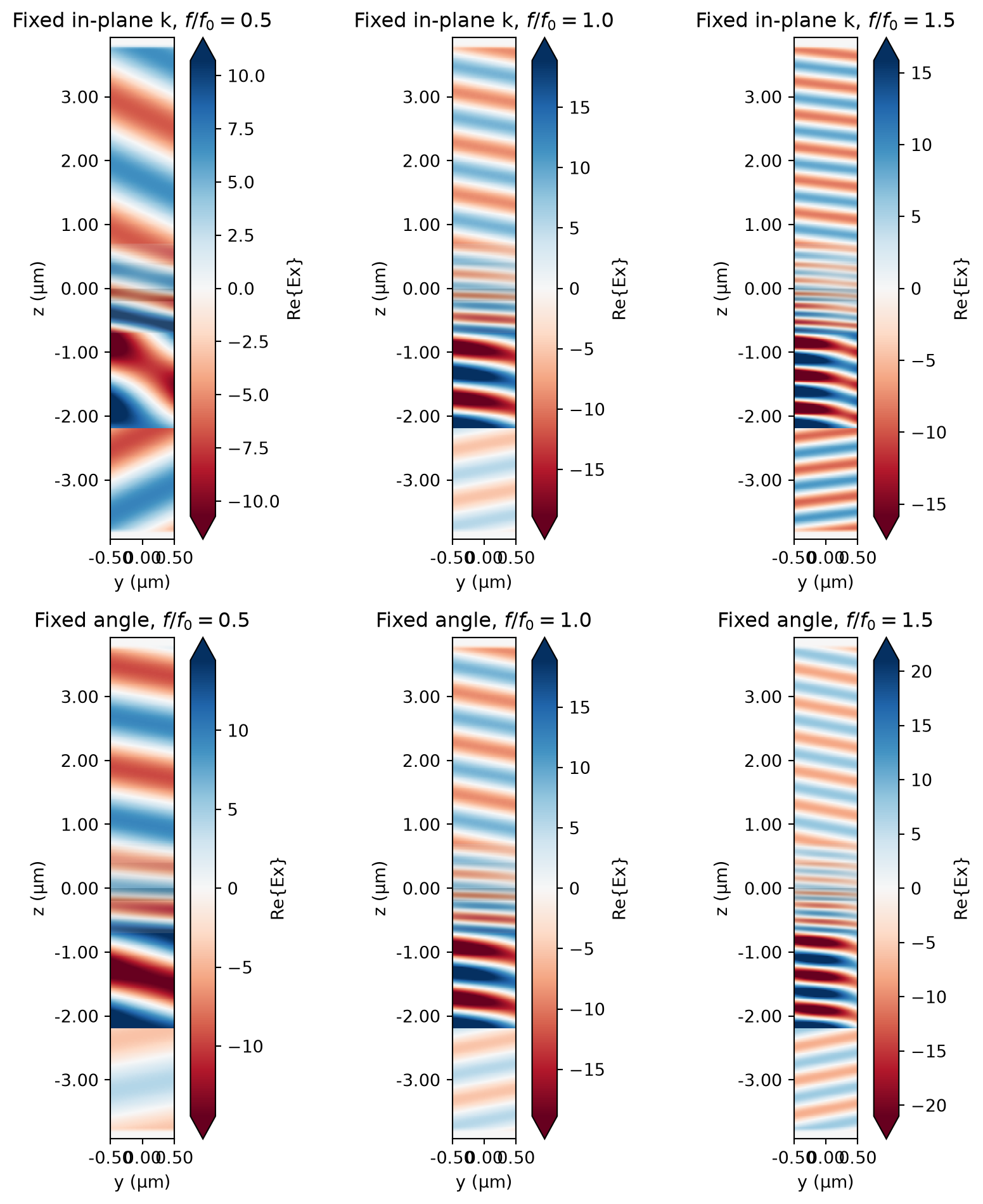
To analyze the simulation results we will record the total transmitted flux. Additionally, for visual comparison we will record the actual field distributions at three different frequency points: the central frequency of the source and the end points of the frequency range defined above.
As it was mentioned in the introduction, when setting up a fixed in-plane k simulation, one must select the corresponding angular_spec in a PlaneWave source definition, and set up compatible periodic Bloch boundary conditions.
Note that FixedInPlaneKSpec is the default value for field angular_spec. Thus, in the code below one can omit explicitly setting this field.
source from (default) to . Additionally, for the fixed in plane k simulations Bloch boundary conditions must be correctly set up, while for the fixed angle simulations periodic boundary conditions are simply set to Periodic.
When setting up a fixed angle simulation one needs to set angular_spec to FixedAngleSpec in the source definition, and apply simple periodic boundary conditions.
03:25:04 UTC Estimated FlexCredit cost: 0.089. This assumes the FDTD solver runs
             for the full simulation time; if early shutoff is reached, the
             billed cost can be lower. Use 'web.real_cost(task_id)' to get the
             billed FlexCredit cost after a simulation run.
             Created task 'fixed_k' with resource_id
             'fdve-f0c9b1bc-9ea9-4445-b6c0-96d4195476e0' and task_type 'FDTD'.
03:25:05 UTC Estimated FlexCredit cost: 0.042. This assumes the FDTD solver runs
             for the full simulation time; if early shutoff is reached, the
             billed cost can be lower. Use 'web.real_cost(task_id)' to get the
             billed FlexCredit cost after a simulation run.
Before submitting the simulations to our servers for solving, let us compare the estimated simulation costs.
03:25:06 UTC Estimated FlexCredit cost: 0.089. This assumes the FDTD solver runs
             for the full simulation time; if early shutoff is reached, the
             billed cost can be lower. Use 'web.real_cost(task_id)' to get the
             billed FlexCredit cost after a simulation run.
03:25:07 UTC Estimated FlexCredit cost: 0.042. This assumes the FDTD solver runs
             for the full simulation time; if early shutoff is reached, the
             billed cost can be lower. Use 'web.real_cost(task_id)' to get the
             billed FlexCredit cost after a simulation run.
Thus, in this particular situation the fixed angle simulation would be approximately charged more by a factor of
cost_fixed_angle / cost_fixed_k
2.1015297615954602
Submit and run simulations as usual.
# Run simulationssim_data_fixed_angle = web.run(simulation=sim_fixed_angle, task_name="fixed_angle")sim_data_fixed_k = web.run(simulation=sim_fixed_k, task_name="fixed_k")
             Created task 'fixed_angle' with resource_id
             'fdve-e0b8b341-e436-4d85-8d05-218b52677669' and task_type 'FDTD'.
03:25:09 UTC Estimated FlexCredit cost: 0.089. This assumes the FDTD solver runs
             for the full simulation time; if early shutoff is reached, the
             billed cost can be lower. Use 'web.real_cost(task_id)' to get the
             billed FlexCredit cost after a simulation run.
03:25:10 UTC status = success
03:25:22 UTC Loading results from simulation_data.hdf5
             Created task 'fixed_k' with resource_id
             'fdve-5e87b55f-ecde-490f-89d6-962a2fa83742' and task_type 'FDTD'.
03:25:24 UTC Estimated FlexCredit cost: 0.042. This assumes the FDTD solver runs
             for the full simulation time; if early shutoff is reached, the
             billed cost can be lower. Use 'web.real_cost(task_id)' to get the
             billed FlexCredit cost after a simulation run.
status = success
03:25:26 UTC Loading results from simulation_data.hdf5
             WARNING: Simulation final field decay value of 3.48e-07 is greater
             than the simulation shutoff threshold of 1e-07. Consider running
             the simulation again with a larger 'run_time' duration for more
             accurate results.
Simulation results analysis
We start the analysis of simulation results with a visual inspection of field distributions recorded at three different frequencies. In the code below, we plot the fixed in-plane k simulation results in the top row and the fixed angle simulation results in the second row.
As one can see, in the fixed in-plane k case the angle of propagating plane wave changes significantly from one frequency point to another one. While in the fixed angle case the simulated plane wave propagation is performed for the same angle.
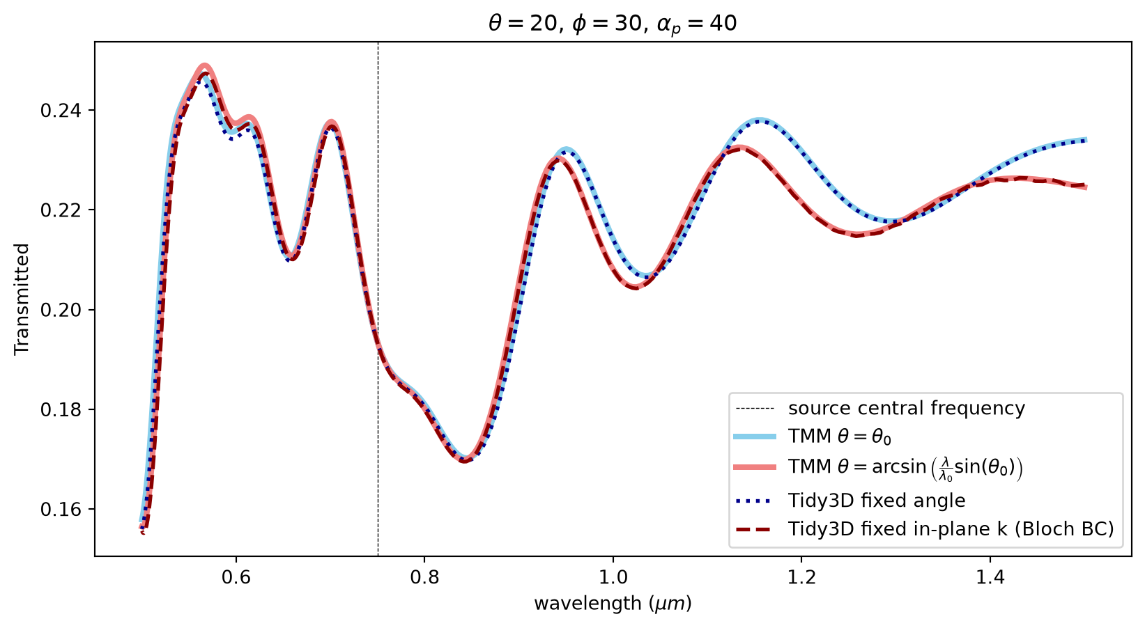
Now we perform a quantitative analysis by comparing simulation results for the transmission flux to values obtained by the Transfer Matrix Method. The code below computes expected transmission fluxes using tmm package.
# Compare to TMMimport tmm# prepare list of thicknesses including air boundariesd_list = [np.inf] + t_slabs + [np.inf]# convert the complex permittivities at each frequency to refractive indicesn_list0 = np.sqrt(mat0.eps_model(monitor_freqs))n_list1 = np.sqrt(mat_slabs[0].eps_model(monitor_freqs))n_list2 = np.sqrt(mat_slabs[1].eps_model(monitor_freqs))n_list3 = np.sqrt(mat_slabs[2].eps_model(monitor_freqs))n_list4 = np.sqrt(mat_slabs[3].eps_model(monitor_freqs))# loop through wavelength and record TMM computed transmissiontransmission_tmm_fixed_k = []transmission_tmm_fixed_angle = []for i, lam inenumerate(monitor_lambdas): theta_fixed_k = np.arcsin(np.sin(theta) * lam * freq0 / td.C_0)# create list of refractive index at this wavelength including outer material (air) n_list = [n_list0[i], n_list1[i], n_list2[i], n_list3[i], n_list4[i], n_list0[i]]# get transmission for fixed angle T = ( tmm.coh_tmm("p", n_list, d_list, theta, lam)["T"] * np.cos(pol) **2+ tmm.coh_tmm("s", n_list, d_list, theta, lam)["T"] * np.sin(pol) **2 ) transmission_tmm_fixed_angle.append(T)# get transmission for fixed in-plane k T = ( tmm.coh_tmm("p", n_list, d_list, theta_fixed_k, lam)["T"] * np.cos(pol) **2+ tmm.coh_tmm("s", n_list, d_list, theta_fixed_k, lam)["T"] * np.sin(pol) **2 ) transmission_tmm_fixed_k.append(T)
These values correspond to the data record by the flux monitors. The code below plot the comparison between the TMM results and the Tidy3D simulation results.
As expected the fixed in-plane k and fixed angle results coincide near the central frequency, but follow different frequency dependencies away from it.
We use necessary cookies to run this website. With your permission, we
also use analytics cookies to understand site usage and marketing
cookies for advertising, retargeting, and HubSpot tracking.
Learn more about our cookie policy.
Privacy choices
Choose which optional cookies Flexcompute may use. Necessary cookies
are always on because they support core website behavior, security, and
saving your consent record.
Your browser is sending a Global Privacy Control signal, so marketing
cookies are disabled.
Subscribe
Thanks for subscribing
Publish Your Notebook
Thank you for publishingA confirmation email has been sent to your inbox. Your notebook will be available within the next 48 hours.
Community Library
TERMS & CONDITIONS
EFFECTIVE DATE: January 1, 2025
Terms and Conditions for User-Submitted Content
By submitting content to Flexcompute, you agree to the following terms:
1. Ownership and Copyright
All content, including but not limited to text, data, images, and other materials submitted by users,
remains the sole property of the original creator. Flexcompute does not claim ownership of the submitted
content or any intellectual property rights associated with it.
Users affirm that they own the copyright or have obtained all necessary permissions for the submitted
content and are fully responsible for ensuring that their submissions do not infringe on any third-party
rights.
2. Responsibility for Content
Users are solely responsible for the content they submit. Flexcompute does not endorse, guarantee,
or verify the accuracy, legality, or appropriateness of any submitted content. Users are responsible
for ensuring that their content complies with all applicable laws and regulations.
Users declare that they have obtained authorization from all co-authors and collaborators associated
with the submitted content, granting them the right to submit and sign on behalf of all contributors.
Users agree not to submit content that is illegal, defamatory, obscene, or violates the rights
of others, including privacy and intellectual property rights.
3. Modification and Presentation
Flexcompute reserves the right to review, edit, or modify submitted content to improve clarity,
formatting, and presentation while maintaining the original intent and message.
These modifications are made to enhance the overall quality and readability of the published material.
Users acknowledge that Flexcompute may format or present the content in a way
that aligns with our editorial and visual standards.
4. Liability Disclaimer
Flexcompute shall not be held liable for any disputes arising from user-submitted content, including
but not limited to copyright claims, inaccuracies, or damages resulting from the publication of user content.
Users agree to indemnify Flexcompute against any claims or legal actions resulting from their submitted content.
5. Content Use Rights
By submitting content, users grant Flexcompute a non-exclusive, royalty-free, worldwide license to publish, distribute,
and promote the content for the purposes of showcasing user contributions and marketing our services.
This license does not transfer ownership of the content or any copyright to Flexcompute.
Users retain the right to withdraw their submissions at any time.
Upon request, Flexcompute will remove the content from its platform.
6. Privacy and Confidentiality
Users acknowledge that submitted content may be publicly accessible and therefore waive any
rights to confidentiality or privacy regarding the published material.
Flexcompute will not share personal information of users without
their consent, in accordance with our privacy policy.
Community Library
How the process works:
You submit your notebook.
You will get a permanent URL to promote your work.
Cite the URL as a reference for others in your upcoming papers to enhance the impact.
When someone clicks your URL, your notebook will be displayed.
Enter your email address below to receive the presentation slides. In the future, we’ll share you very few emails when we have new tutorial release, development updates, valuable toolkits and technical guidance . You can unsubscribe at any time by clicking the link at the bottom of every email. We’ll never share your information.








 TERMS & CONDITIONS


 How the process works:
 Try this real URL to see an example: