





import matplotlib.pyplot as plt
import numpy as np
import tidy3d as td
import tidy3d.web as web
from matplotlib.colors import Normalize
TIDY3D
LEARNING CENTER
Example Library

Ultrasensitive biosensing with 3D quasi-BIC metasurfaces
This notebook demonstrates a Tidy3D implementation inspired by selected simulations from J. Sun et al., Nature Photonics (2026) DOI: 10.1038/s41566-026-01909-z.
The paper introduces Q-modulated refractometric sensing (QMRS) using a strongly coupled three-dimensional quasi-bound-state-in-the-continuum (qBIC) metasurface. Each unit cell contains two nominally identical Au/TiO₂-coated resonators positioned at different vertical depths. Their coupling produces lower and upper hybrid branches, qBICL and qBICU, with distinct responses to a superstrate refractive-index perturbation. The more localized qBICL branch behaves primarily as a conventional refractometric mode and shifts in frequency. In contrast, the more non-local qBICU branch has weaker direct analyte overlap but exhibits pronounced radiative-Q and intensity modulation with relatively little frequency shift.
Model assumptions and relation to the paper:
- Both models use FDTD simulations with periodic boundaries in \(x\) and \(y\), perfectly matched layers along \(z\), and normal-incidence plane-wave illumination.
- The paper uses a uniform 5 nm mesh. This notebook instead uses Tidy3D’s automatic nonuniform grid with 30 steps per wavelength, selected following an independent convergence study spanning 15–40 steps per wavelength.
- Au is modeled using the Johnson–Christy (1972) dispersive model. The nondispersive refractive indices are \(n_\mathrm{NOA83}=1.56\), \(n_\mathrm{TiO_2}=2.20\), and \(n_\mathrm{sup}=1.33+\Delta n\).
- Unless otherwise stated, the geometric dimensions below are simulation inputs used in this notebook and may not exactly match those reported in the paper.
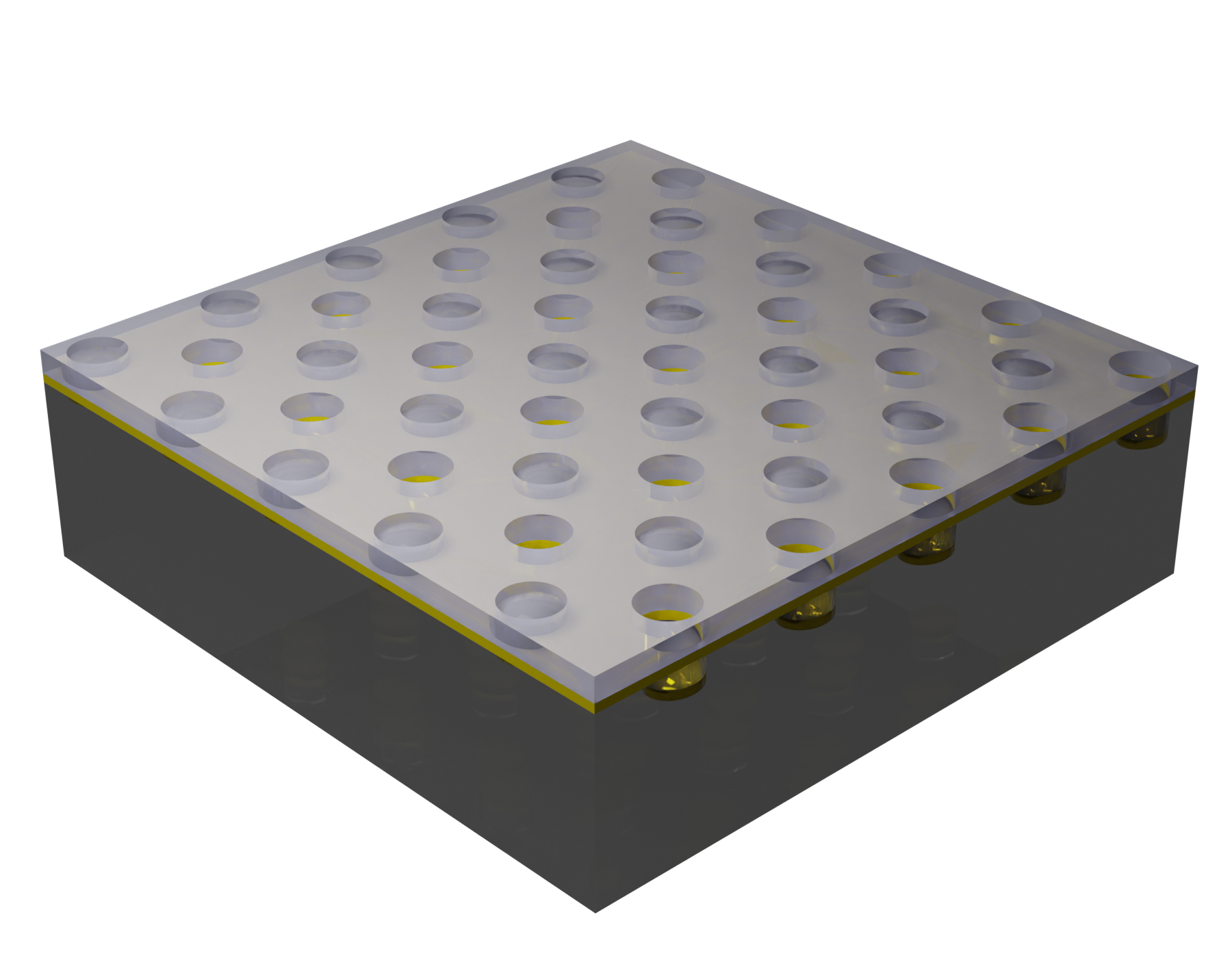
Simulation Setup
SWIR Device Parameters
The parameters below model the paper’s short-wave-infrared design (\(P=800\) nm) over 0.84–1.02 eV (approximately 1.22–1.48 µm). All geometric quantities are expressed in micrometres, the native length unit in Tidy3D. Photon energies are converted to frequencies through \(E=2\pi\hbar f\).
# Spectral range — SWIR device
photon_energy_min = 0.84  # eV
photon_energy_max = 1.02  # eV

P = 0.8  # unit cell period (µm)
P2 = P * np.sqrt(2)  # doubled supercell period (µm)

fmin = photon_energy_min / td.HBAR / (2 * np.pi)
fmax = photon_energy_max / td.HBAR / (2 * np.pi)
freq0 = (fmin + fmax) / 2
fwidth = fmax - fmin
wvl0 = td.C_0 / freq0

freqs = np.linspace(fmin, fmax, 241)
source_time = td.GaussianPulse(freq0=freq0, fwidth=fwidth)

nm = 1e-3  # nanometre in Tidy3D units (µm)

# Materials
Au = td.material_library["Au"]["JohnsonChristy1972"]
TiO2 = td.Medium.from_nk(n=2.2, k=0, freq=freq0)
NOA83 = td.Medium.from_nk(n=1.56, k=0, freq=freq0)

wvl_eff = wvl0 / NOA83.nk_model(frequency=freq0)[0]  # effective wavelength in substrate
wvl_water = wvl0 / 1.33  # effective wavelength in substrate

# Base geometry (µm) — passed explicitly to make_sim / make_sim2
D_A = 300 * nm  # particle-A diameter
D_B = D_A  # particle-B diameter (symmetric base case)
Z_A = 200 * nm  # particle-A hole depth
del_Z = 120 * nm
Z_B = Z_A - del_Z  # particle-B hole depth

buffer = 0.2
sim_size_z_plus = (
    buffer + 1 * wvl_water
)  # simulation size in z direction (used as global inside make_sim / make_sim2)
sim_size_z_minus = (
    buffer + 3 * wvl_eff
)  # simulation size in z direction (used as global inside make_sim / make_sim2)
Unit Cell Simulation
The primitive square cell contains one A site and one B site. Au and TiO₂ conformal layers occupy cylindrical recesses in the NOA83 substrate and continue across the top surface. A normally incident, \(x\)-polarized plane wave propagates from the substrate toward the aqueous superstrate.
def make_sim(
    D_A: float = 0.3,
    D_B: float = 0.3,
    Z_A: float = 0.2,
    Z_B: float = 0.08,
    t_TiO2: float = 130e-3,
    t_Au: float = 50e-3,
    deln_bulk: float = 0.0,
    min_steps_per_wvl: int = 30,
) -> td.Simulation:
    """Primitive-cell FDTD simulation.

    Parameters (all lengths in µm):
        D_A, D_B        : nanohole diameters for particles A and B
        Z_A, Z_B        : nanohole depths for particles A and B
        t_TiO2, t_Au    : TiO₂ and Au film thicknesses
        deln_bulk       : superstrate refractive-index offset from n=1.33
        min_steps_per_wvl: auto-grid resolution
    """
    hole_A = td.Cylinder(
        axis=2, center=(P / 4, P / 4, -Z_A / 2), radius=D_A / 2, length=Z_A
    )
    hole_B = td.Cylinder(
        axis=2, center=(-P / 4, -P / 4, -Z_B / 2), radius=D_B / 2, length=Z_B
    )

    geom_sub = td.ClipOperation(
        operation="difference",
        geometry_a=td.Box(
            center=(0, 0, -sim_size_z_minus),
            size=(td.inf, td.inf, sim_size_z_minus * 2),
        ),
        geometry_b=td.GeometryGroup(geometries=[hole_A, hole_B]),
    )
    substrate = td.Structure(geometry=geom_sub, medium=NOA83, name="substrate")

    deposit_au_A = td.Structure(
        geometry=td.Cylinder(
            axis=2, center=(P / 4, P / 4, -Z_A + t_Au / 2), radius=D_A / 2, length=t_Au
        ),
        medium=Au,
        name="au_A",
    )
    deposit_au_B = td.Structure(
        geometry=td.Cylinder(
            axis=2,
            center=(-P / 4, -P / 4, -Z_B + t_Au / 2),
            radius=D_B / 2,
            length=t_Au,
        ),
        medium=Au,
        name="au_B",
    )
    deposit_au_sub = td.Structure(
        geometry=td.ClipOperation(
            operation="difference",
            geometry_a=td.Box(center=(0, 0, t_Au / 2), size=(td.inf, td.inf, t_Au)),
            geometry_b=td.GeometryGroup(
                geometries=[
                    td.Cylinder(
                        axis=2,
                        center=(-P / 4, -P / 4, t_Au / 2),
                        radius=D_B / 2,
                        length=t_Au,
                    ),
                    td.Cylinder(
                        axis=2,
                        center=(P / 4, P / 4, t_Au / 2),
                        radius=D_A / 2,
                        length=t_Au,
                    ),
                ]
            ),
        ),
        medium=Au,
        name="au_sub",
    )
    deposit_au = [deposit_au_A, deposit_au_B, deposit_au_sub]

    deposit_tio2_A = td.Structure(
        geometry=td.Cylinder(
            axis=2,
            center=(P / 4, P / 4, -Z_A + t_Au + t_TiO2 / 2),
            radius=D_A / 2,
            length=t_TiO2,
        ),
        medium=TiO2,
        name="TiO2_A",
    )
    deposit_tio2_B = td.Structure(
        geometry=td.Cylinder(
            axis=2,
            center=(-P / 4, -P / 4, -Z_B + t_Au + t_TiO2 / 2),
            radius=D_B / 2,
            length=t_TiO2,
        ),
        medium=TiO2,
        name="TiO2_B",
    )
    deposit_tio2_sub = td.Structure(
        geometry=td.ClipOperation(
            operation="difference",
            geometry_a=td.Box(
                center=(0, 0, t_Au + t_TiO2 / 2), size=(td.inf, td.inf, t_TiO2)
            ),
            geometry_b=td.GeometryGroup(
                geometries=[
                    td.Cylinder(
                        axis=2,
                        center=(-P / 4, -P / 4, t_Au + t_TiO2 / 2),
                        radius=D_B / 2,
                        length=t_TiO2,
                    ),
                    td.Cylinder(
                        axis=2,
                        center=(P / 4, P / 4, t_Au + t_TiO2 / 2),
                        radius=D_A / 2,
                        length=t_TiO2,
                    ),
                ]
            ),
        ),
        medium=TiO2,
        name="TiO2_sub",
    )
    deposit_tio2 = [deposit_tio2_A, deposit_tio2_B, deposit_tio2_sub]

    pw_source = td.PlaneWave(
        center=(0, 0, -buffer - 0.5 * wvl_eff),
        size=(td.inf, td.inf, 0),
        direction="+",
        source_time=source_time,
        pol_angle=0,
    )
    mnt_refl = td.FluxMonitor(
        center=(0, 0, -buffer - wvl_eff),
        size=(td.inf, td.inf, 0),
        freqs=freqs,
        name="refl",
        normal_dir="-",
    )
    mnt_trans = td.FluxMonitor(
        center=(0, 0, buffer + 0.5 * wvl_water),
        size=(td.inf, td.inf, 0),
        freqs=freqs,
        name="trans",
        normal_dir="+",
    )

    superstrate = td.Medium.from_nk(n=1.33 + deln_bulk, k=0.0, freq=freq0)

    grid_spec = td.GridSpec.auto(
        wavelength=wvl0,
        min_steps_per_wvl=min_steps_per_wvl,
        snapping_points=[
            (P / 4, P / 4, pw_source.center[2]),
            (-P / 4, -P / 4, mnt_refl.center[2]),
            (0, 0, mnt_trans.center[2]),
        ],
    )

    return td.Simulation(
        size=(P, P, sim_size_z_plus + sim_size_z_minus),
        center=(0, 0, (sim_size_z_plus - sim_size_z_minus) / 2),
        medium=superstrate,
        structures=[substrate, *deposit_au, *deposit_tio2],
        sources=[pw_source],
        monitors=[mnt_refl, mnt_trans],
        grid_spec=grid_spec,
        boundary_spec=td.BoundarySpec(
            z=td.Boundary.pml(),
            x=td.Boundary.periodic(),
            y=td.Boundary.periodic(),
        ),
        run_time=td.RunTimeSpec(quality_factor=500, source_factor=100),
        shutoff=5e-7,
    )
The 3D structure and computational grid of the base simulation are shown below.
sim_base = make_sim()

fig, ax = plt.subplots()
sim_base.plot_grid(x=P / 4, ax=ax)
sim_base.plot(x=P / 4, ax=ax)
ax.set(
    xlim=(-P / 2, P / 2), ylim=(-P / 2, P / 2), title="Cross-section through particle A"
)

sim_base.plot_3d()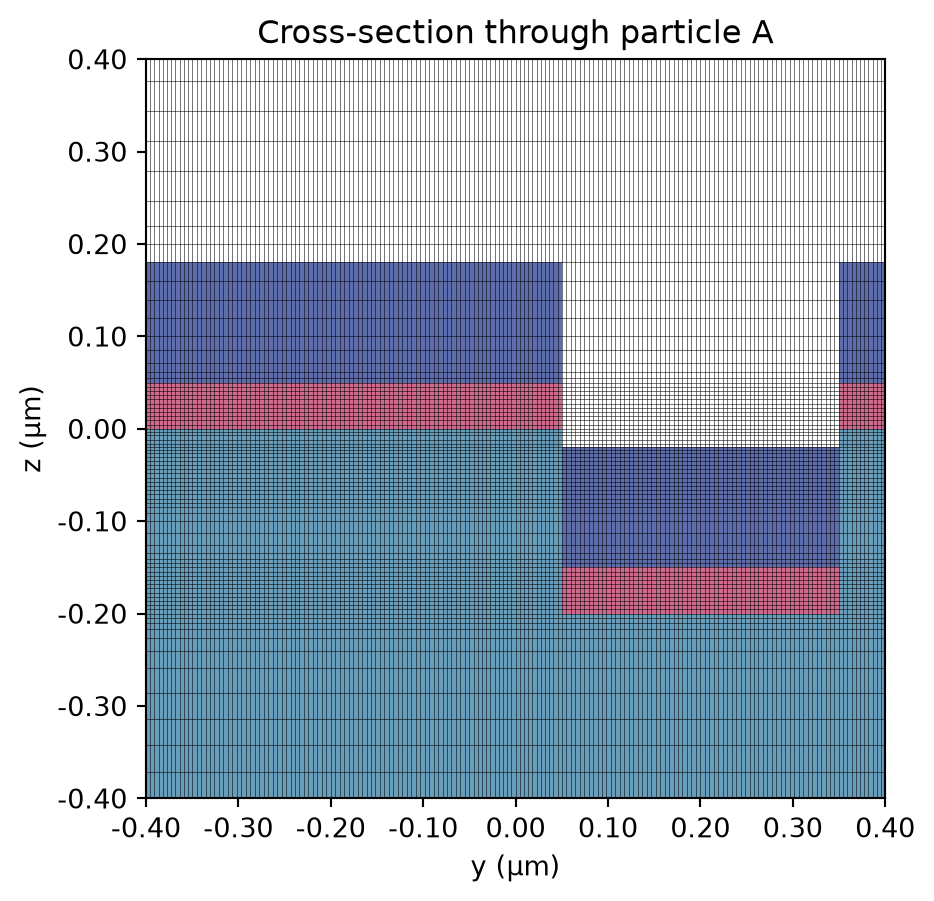
Grid Convergence Test
This implementation uses Tidy3D’s automatic nonuniform grid. We therefore first perform a grid-convergence study to verify that the simulated spectral response is insensitive to further mesh refinement.
sims = {f"{n}-step": make_sim(min_steps_per_wvl=n) for n in [15, 20, 25, 30, 35, 40]}

batch_data = web.run_async(
    simulations=sims, verbose=True, folder_name="NatPhoton2026", path_dir="./data/conv"
)
10:24:06 UTC WARNING: Suppressed 1 WARNING message.
             WARNING: Simulation has 2.21e+06 time steps. The 'run_time' may be
             unnecessarily large, unless there are very long-lived resonances.
             WARNING: Simulation has 1.87e+06 time steps. The 'run_time' may be
             unnecessarily large, unless there are very long-lived resonances.
             WARNING: Simulation has 1.43e+06 time steps. The 'run_time' may be
             unnecessarily large, unless there are very long-lived resonances.
             WARNING: Simulation has 1.96e+06 time steps. The 'run_time' may be
             unnecessarily large, unless there are very long-lived resonances.
             WARNING: Simulation has 1.23e+06 time steps. The 'run_time' may be
             unnecessarily large, unless there are very long-lived resonances.
10:24:39 UTC Started working on Batch containing 6 tasks.
10:24:45 UTC Maximum FlexCredit cost: 24.200 for the whole batch.
             Use 'Batch.real_cost()' to get the billed FlexCredit cost after
             completion.
Reflectance and transmittance fluxes are used to compute the absorptance, \(A = 1 - R - T\). The absorption spectra are compared across six automatic-grid resolutions spanning 15–40 steps per wavelength. Based on this comparison, the 30-steps-per-wavelength grid is selected and used throughout the remainder of this notebook.
fig, ax = plt.subplots()
cmap = plt.cm.viridis
n_steps = [15, 20, 25, 30, 35, 40]
norm = Normalize(vmin=15, vmax=40)
for n in n_steps:
    sim_data = batch_data[f"{n}-step"]
    refl = sim_data["refl"].flux.squeeze()
    trans = sim_data["trans"].flux.squeeze()
    abs_spec = 1 - refl - trans
    f = abs_spec.f
    ax.plot(
        2 * np.pi * f * td.HBAR,
        abs_spec,
        "-",
        lw=1.5 if n == 30 else 1,
        color=cmap(norm(n)),
    )

ax.set(
    xlabel="Frequency (eV)",
    ylabel="Absorption",
    ylim=(0, 1),
    xlim=(photon_energy_min, photon_energy_max),
)

sm = plt.cm.ScalarMappable(cmap=cmap, norm=norm)
sm.set_array([])
cbar = fig.colorbar(sm, ax=ax)
cbar.set_label(r"# steps per wavelength")
cbar.set_ticks(n_steps)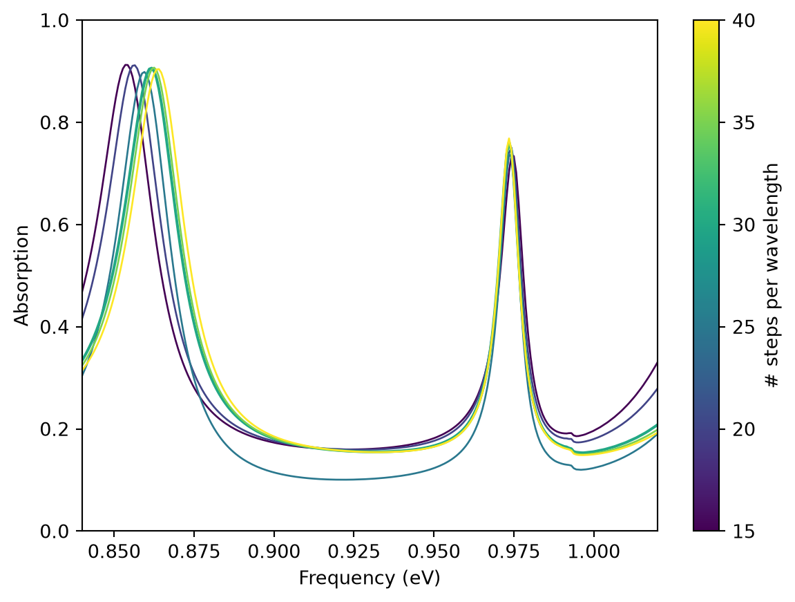
Effect of Asymmetry
In-plane Symmetry Breaking: Diameter Asymmetry
With \(Z_A=Z_B=200\) nm, the diameter difference \(\Delta D=D_A-D_B\) is swept from 0 to 260 nm by holding \(D_A=300\) nm and decreasing \(D_B\). At \(\Delta D=0\), the symmetry-protected mode is ideally dark at normal incidence. A nonzero \(\Delta D\) breaks the in-plane symmetry, opens radiative coupling, and produces finite-linewidth qBIC resonances. As emphasized in the paper, diameter asymmetry also perturbs the individual resonators and therefore causes eigenfrequency shifts and interbranch crosstalk.
delD_list = np.linspace(0, 260 * nm, 14)
sims = {
    f"deld_sweep_{ii}": make_sim(
        Z_A=200 * nm, Z_B=200 * nm, D_A=300 * nm, D_B=300 * nm - deld
    )
    for ii, deld in enumerate(delD_list)
}

batch_data = web.run_async(
    simulations=sims,
    verbose=True,
    folder_name="NatPhoton2026",
    path_dir="./data/diameter",
)
10:53:14 UTC WARNING: Simulation has 1.70e+06 time steps. The 'run_time' may be unnecessarily large, unless there are very long-lived resonances.
             WARNING: Simulation has 1.70e+06 time steps. The 'run_time' may be
             unnecessarily large, unless there are very long-lived resonances.
             WARNING: Simulation has 1.70e+06 time steps. The 'run_time' may be
             unnecessarily large, unless there are very long-lived resonances.
             WARNING: Simulation has 1.70e+06 time steps. The 'run_time' may be
             unnecessarily large, unless there are very long-lived resonances.
             WARNING: Simulation has 1.70e+06 time steps. The 'run_time' may be
             unnecessarily large, unless there are very long-lived resonances.
             WARNING: Simulation has 1.70e+06 time steps. The 'run_time' may be
             unnecessarily large, unless there are very long-lived resonances.
             WARNING: Simulation has 1.70e+06 time steps. The 'run_time' may be
             unnecessarily large, unless there are very long-lived resonances.
             WARNING: Simulation has 1.70e+06 time steps. The 'run_time' may be
             unnecessarily large, unless there are very long-lived resonances.
             WARNING: Simulation has 1.73e+06 time steps. The 'run_time' may be
             unnecessarily large, unless there are very long-lived resonances.
             WARNING: Simulation has 1.85e+06 time steps. The 'run_time' may be
             unnecessarily large, unless there are very long-lived resonances.
             WARNING: Simulation has 1.70e+06 time steps. The 'run_time' may be
             unnecessarily large, unless there are very long-lived resonances.
             WARNING: Simulation has 1.70e+06 time steps. The 'run_time' may be
             unnecessarily large, unless there are very long-lived resonances.
             WARNING: Simulation has 1.77e+06 time steps. The 'run_time' may be
             unnecessarily large, unless there are very long-lived resonances.
             WARNING: Simulation has 1.70e+06 time steps. The 'run_time' may be
             unnecessarily large, unless there are very long-lived resonances.
10:53:22 UTC Started working on Batch containing 14 tasks.
10:53:34 UTC Maximum FlexCredit cost: 52.905 for the whole batch.
             Use 'Batch.real_cost()' to get the billed FlexCredit cost after
             completion.
fig, ax = plt.subplots()
cmap = plt.cm.cividis
norm = Normalize(vmin=0, vmax=260)
for ii, deld in enumerate(delD_list):
    sim_data = batch_data[f"deld_sweep_{ii}"]
    refl = sim_data["refl"].flux.squeeze()
    trans = sim_data["trans"].flux.squeeze()
    abs_spec = 1 - refl - trans
    f = refl.f
    ax.plot(2 * np.pi * f * td.HBAR, abs_spec, "-", lw=1, color=cmap(norm(deld * 1e3)))

ax.set(
    xlabel="Frequency (eV)",
    ylabel="Absorption",
    ylim=(0, 1),
    xlim=(photon_energy_min, photon_energy_max),
)

sm = plt.cm.ScalarMappable(cmap=cmap, norm=norm)
sm.set_array([])
cbar = fig.colorbar(sm, ax=ax)
cbar.set_label(r"$\Delta D$ (nm)")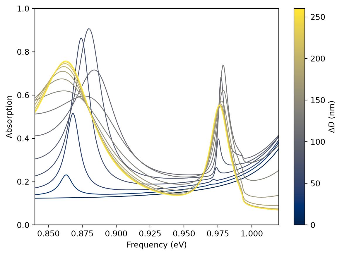
Out-of-plane Symmetry Breaking: Vertical Displacement
With \(D_A=D_B=300\) nm and \(Z_A=200\) nm, the vertical displacement \(\Delta Z=Z_A-Z_B\) is swept from 0 to 130 nm. A nonzero \(\Delta Z\) breaks the out-of-plane symmetry and opens controlled radiative channels, making the lower and upper hybrid branches observable as qBIC_L and qBIC_U. Crucially, \(\Delta Z\) primarily controls radiative leakage and linewidth; it does not by itself create the strong coupling or Rabi splitting. The paper contrasts this comparatively stable eigenfrequency tuning with the stronger modal crosstalk produced by diameter asymmetry.
delZ_list = np.linspace(0, 130 * nm, 14)
sims = {
    f"delz_sweep_{ii}": make_sim(Z_A=200 * nm, Z_B=200 * nm - delz)
    for ii, delz in enumerate(delZ_list)
}

batch_data = web.run_async(
    simulations=sims, verbose=True, folder_name="NatPhoton2026", path_dir="./data/depth"
)
11:22:54 UTC Got 1 simulation from cache.
             WARNING: Simulation has 1.70e+06 time steps. The 'run_time' may be
             unnecessarily large, unless there are very long-lived resonances.
             WARNING: Simulation has 1.87e+06 time steps. The 'run_time' may be
             unnecessarily large, unless there are very long-lived resonances.
             WARNING: Simulation has 1.73e+06 time steps. The 'run_time' may be
             unnecessarily large, unless there are very long-lived resonances.
             WARNING: Simulation has 1.73e+06 time steps. The 'run_time' may be
             unnecessarily large, unless there are very long-lived resonances.
             WARNING: Simulation has 1.87e+06 time steps. The 'run_time' may be
             unnecessarily large, unless there are very long-lived resonances.
             WARNING: Simulation has 1.70e+06 time steps. The 'run_time' may be
             unnecessarily large, unless there are very long-lived resonances.
             WARNING: Simulation has 1.87e+06 time steps. The 'run_time' may be
             unnecessarily large, unless there are very long-lived resonances.
             WARNING: Simulation has 1.87e+06 time steps. The 'run_time' may be
             unnecessarily large, unless there are very long-lived resonances.
             WARNING: Simulation has 1.87e+06 time steps. The 'run_time' may be
             unnecessarily large, unless there are very long-lived resonances.
             WARNING: Simulation has 1.70e+06 time steps. The 'run_time' may be
             unnecessarily large, unless there are very long-lived resonances.
             WARNING: Simulation has 1.73e+06 time steps. The 'run_time' may be
             unnecessarily large, unless there are very long-lived resonances.
             WARNING: Simulation has 1.70e+06 time steps. The 'run_time' may be
             unnecessarily large, unless there are very long-lived resonances.
             WARNING: Simulation has 1.73e+06 time steps. The 'run_time' may be
             unnecessarily large, unless there are very long-lived resonances.
11:23:01 UTC Started working on Batch containing 14 tasks.
11:23:12 UTC Maximum FlexCredit cost: 52.913 for the whole batch.
             Use 'Batch.real_cost()' to get the billed FlexCredit cost after
             completion.
fig, ax = plt.subplots()
cmap = plt.cm.cividis
norm = Normalize(vmin=0, vmax=130)
for ii, delz in enumerate(delZ_list):
    sim_data = batch_data[f"delz_sweep_{ii}"]
    refl = sim_data["refl"].flux.squeeze()
    trans = sim_data["trans"].flux.squeeze()
    abs_spec = 1 - refl - trans
    f = refl.f
    ax.plot(2 * np.pi * f * td.HBAR, abs_spec, "-", lw=1, color=cmap(norm(delz * 1e3)))

ax.set(
    xlabel="Frequency (eV)",
    ylabel="Absorption",
    ylim=(0, 1),
    xlim=(photon_energy_min, photon_energy_max),
)

sm = plt.cm.ScalarMappable(cmap=cmap, norm=norm)
sm.set_array([])
cbar = fig.colorbar(sm, ax=ax)
cbar.set_label(r"$\Delta Z$ (nm)")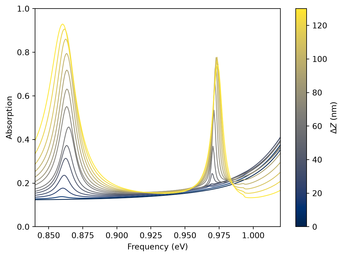
Bulk Refractive-index Perturbation
The simulation geometry is \(Z_A=194\) nm, \(Z_B=30\) nm, and \(t_\mathrm{TiO_2}=60\) nm. The aqueous-superstrate perturbation is swept from \(\Delta n=0\) to 0.08 RIU.
deln_list = np.linspace(0, 0.08, 9)
sims = {
    f"deln_sweep_{ii}": make_sim(
        Z_A=194 * nm, Z_B=30 * nm, t_TiO2=60 * nm, deln_bulk=deln
    )
    for ii, deln in enumerate(deln_list)
}

batch_data = web.run_async(
    simulations=sims,
    verbose=True,
    folder_name="NatPhoton2026",
    path_dir="./data/deltan",
)
11:42:31 UTC WARNING: Simulation has 1.73e+06 time steps. The 'run_time' may be unnecessarily large, unless there are very long-lived resonances.
             WARNING: Simulation has 1.73e+06 time steps. The 'run_time' may be
             unnecessarily large, unless there are very long-lived resonances.
             WARNING: Simulation has 1.74e+06 time steps. The 'run_time' may be
             unnecessarily large, unless there are very long-lived resonances.
             WARNING: Simulation has 1.73e+06 time steps. The 'run_time' may be
             unnecessarily large, unless there are very long-lived resonances.
WARNING: Suppressed 1 WARNING message.
             WARNING: Simulation has 1.74e+06 time steps. The 'run_time' may be
             unnecessarily large, unless there are very long-lived resonances.
             WARNING: Simulation has 1.73e+06 time steps. The 'run_time' may be
             unnecessarily large, unless there are very long-lived resonances.
             WARNING: Simulation has 1.74e+06 time steps. The 'run_time' may be
             unnecessarily large, unless there are very long-lived resonances.
             WARNING: Simulation has 1.74e+06 time steps. The 'run_time' may be
             unnecessarily large, unless there are very long-lived resonances.
11:43:05 UTC Started working on Batch containing 9 tasks.
11:43:13 UTC Maximum FlexCredit cost: 35.009 for the whole batch.
             Use 'Batch.real_cost()' to get the billed FlexCredit cost after
             completion.
12:02:04 UTC Batch complete.
Dashed lines mark the independently extracted qBIC_L and qBIC_U absorption peaks at both endpoints.
peak_frequencies_from_derivatives identifies peak frequencies from local maxima of the absorption spectrum: candidates are points where \(dA/df\) changes from positive to negative and \(d^2A/df^2<0\). If the sampled spectrum misses one sign change, the helper falls back to interior negative-curvature regions and chooses the point with the smallest \(|dA/df|\). Only the endpoint frequencies \(f_{L0}\), \(f_{L1}\), and \(f_U\) are extracted for the near-field simulations.
The local qBIC_L branch has relatively strong field overlap with the superstrate and therefore responds predominantly through a resonance-frequency shift, as in conventional refractometric sensing. The non-local qBIC_U branch has weaker direct analyte overlap and undergoes comparatively little frequency shift, but its radiative loss rate changes strongly. This conversion of a real refractive-index perturbation into an intensity response is the defining QMRS mechanism.
# Peaks are local maxima with negative curvature. Only f_L0, f_L1, and f_U are extracted.
def peak_frequencies_from_derivatives(f, A, n_peaks=2):
    f = np.asarray(f, dtype=float)
    A = np.asarray(A, dtype=float)

    dA_df = np.gradient(A, f)
    d2A_df2 = np.gradient(dA_df, f)

    maxima = np.flatnonzero((dA_df[:-1] > 0) & (dA_df[1:] <= 0))
    candidates = []
    for idx in maxima:
        peak_idx = idx if abs(dA_df[idx]) <= abs(dA_df[idx + 1]) else idx + 1
        if 0 < peak_idx < len(f) - 1 and d2A_df2[peak_idx] < 0:
            candidates.append(peak_idx)

    if len(candidates) < n_peaks:
        valid = d2A_df2 < 0
        valid[:2] = False
        valid[-2:] = False
        idx = np.flatnonzero(valid)
        regions = np.split(idx, np.where(np.diff(idx) > 1)[0] + 1) if len(idx) else []
        for region in regions:
            candidates.append(region[np.argmin(np.abs(dA_df[region]))])

    candidates = np.unique(candidates)
    if len(candidates) < n_peaks:
        raise RuntimeError(f"Found only {len(candidates)} peak candidates.")

    selected = candidates[np.argsort(A[candidates])[-n_peaks:]]
    return np.sort(f[selected])


fig, ax = plt.subplots()
cmap = plt.cm.copper
norm = Normalize(vmin=0, vmax=0.08)

for ii, deln in enumerate(deln_list):
    sim_data = batch_data[f"deln_sweep_{ii}"]
    refl = sim_data["refl"].flux.squeeze()
    trans = sim_data["trans"].flux.squeeze()
    abs_spec = 1 - refl - trans
    f = np.asarray(abs_spec.f)
    E = 2 * np.pi * f * td.HBAR
    A = np.asarray(abs_spec)

    ax.plot(E, A, "-", lw=1, color=cmap(norm(deln)))

    if ii == 0:
        (f_L0,) = peak_frequencies_from_derivatives(f, A, n_peaks=1)
    elif ii == len(deln_list) - 1:
        f_L1, f_U = peak_frequencies_from_derivatives(f, A, n_peaks=2)

ax.set(
    xlabel="Frequency (eV)",
    ylabel="Absorption",
    ylim=(0, 1),
    xlim=(photon_energy_min, photon_energy_max),
)

sm = plt.cm.ScalarMappable(cmap=cmap, norm=norm)
sm.set_array([])
cbar = fig.colorbar(sm, ax=ax)
cbar.set_label(r"Superstrate index change, $\Delta n$")

for fv, label in zip([f_L0, f_L1, f_U], [r"$f_{L0}$", r"$f_{L1}$", r"$f_U$"]):
    E_peak = 2 * np.pi * fv * td.HBAR
    ax.axvline(x=E_peak, color="k", lw=0.75, ls="--")
    ax.text(E_peak + 0.002, 0.9, label, fontsize=12)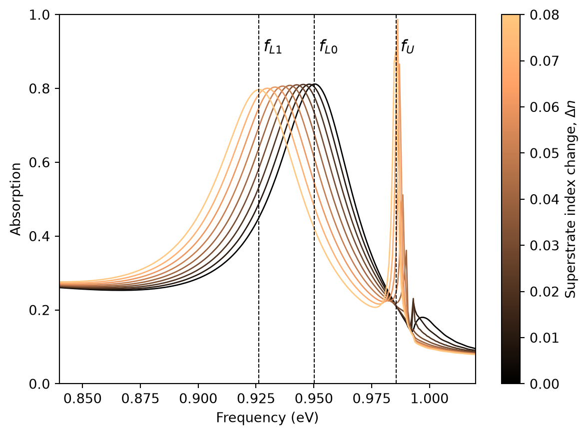
Near-field Response in a Rotated Two-cell Supercell
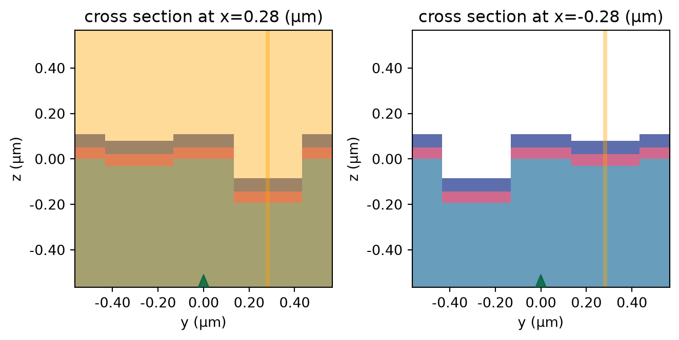
A square domain of side \(P_2=P\sqrt{2}\), rotated by 45° relative to the primitive-cell basis, has area \(2P^2\) and therefore contains two primitive cells: four sites in total. It is consequently a rotated two-cell supercell, not a conventional 2×2 array of four primitive cells. The representation places two A sites and two B sites in one Cartesian periodic domain, making the selected vertical cross-sections convenient for comparing the two site types.
make_sim2 starts from make_sim(**kwargs) and constructs the rotated two-cell geometry with updated_copy. The domain, structures, monitors, and grid snapping points are replaced; the boundary conditions, source, background medium, termination specification, and shutoff threshold are inherited.
Dependency: Run the bulk-index sweep first to obtain the resonance frequencies
f_L0,f_L1, andf_U.
def make_sim2(freqs, **kwargs) -> td.Simulation:
    """2×2 supercell FDTD simulation for near-field visualization.

    Calls ``make_sim(**kwargs)`` for the primitive-cell base, then updates it
    to the supercell via ``updated_copy``: domain size, structures, monitors,
    and snapping points are replaced; boundary conditions, source, medium,
    ``run_time``, and ``shutoff`` are inherited unchanged.

    Parameters:
        freqs : array-like of float
            Monitor frequencies (Hz).
        **kwargs : forwarded to ``make_sim`` (geometry, materials, Δn, grid resolution).
    """
    D_A = kwargs.get("D_A", 0.3)
    D_B = kwargs.get("D_B", 0.3)
    Z_A = kwargs.get("Z_A", 0.2)
    Z_B = kwargs.get("Z_B", 0.08)
    t_Au = kwargs.get("t_Au", 50e-3)
    t_TiO2 = kwargs.get("t_TiO2", 130e-3)
    sim_base = make_sim(**kwargs)

    hole_A1 = td.Cylinder(
        axis=2, center=(P2 / 4, P2 / 4, -Z_A / 2), radius=D_A / 2, length=Z_A
    )
    hole_B1 = td.Cylinder(
        axis=2, center=(P2 / 4, -P2 / 4, -Z_B / 2), radius=D_B / 2, length=Z_B
    )
    hole_A2 = td.Cylinder(
        axis=2, center=(-P2 / 4, -P2 / 4, -Z_A / 2), radius=D_A / 2, length=Z_A
    )
    hole_B2 = td.Cylinder(
        axis=2, center=(-P2 / 4, P2 / 4, -Z_B / 2), radius=D_B / 2, length=Z_B
    )

    geom_sub = td.ClipOperation(
        operation="difference",
        geometry_a=td.Box(
            center=(0, 0, -sim_size_z_minus),
            size=(td.inf, td.inf, sim_size_z_minus * 2),
        ),
        geometry_b=td.GeometryGroup(geometries=[hole_A1, hole_B1, hole_A2, hole_B2]),
    )
    substrate = td.Structure(geometry=geom_sub, medium=NOA83, name="substrate")

    deposit_au = [
        td.Structure(
            geometry=td.Cylinder(
                axis=2,
                center=(
                    s1 * P2 / 4,
                    s2 * P2 / 4,
                    -(Z_A if s1 == s2 else Z_B) + t_Au / 2,
                ),
                radius=(D_A if s1 == s2 else D_B) / 2,
                length=t_Au,
            ),
            medium=Au,
            name=f"au_{s1}_{s2}",
        )
        for s1 in [-1, 1]
        for s2 in [-1, 1]
    ]
    deposit_au_sub = td.Structure(
        geometry=td.ClipOperation(
            operation="difference",
            geometry_a=td.Box(center=(0, 0, t_Au / 2), size=(td.inf, td.inf, t_Au)),
            geometry_b=td.GeometryGroup(
                geometries=[
                    td.Cylinder(
                        axis=2,
                        center=(s1 * P2 / 4, s2 * P2 / 4, t_Au / 2),
                        radius=(D_A if s1 == s2 else D_B) / 2,
                        length=t_Au,
                    )
                    for s1 in [-1, 1]
                    for s2 in [-1, 1]
                ]
            ),
        ),
        medium=Au,
        name="au_sub",
    )

    deposit_tio2 = [
        td.Structure(
            geometry=td.Cylinder(
                axis=2,
                center=(
                    s1 * P2 / 4,
                    s2 * P2 / 4,
                    -(Z_A if s1 == s2 else Z_B) + t_Au + t_TiO2 / 2,
                ),
                radius=(D_A if s1 == s2 else D_B) / 2,
                length=t_TiO2,
            ),
            medium=TiO2,
            name=f"tio2_{s1}_{s2}",
        )
        for s1 in [-1, 1]
        for s2 in [-1, 1]
    ]
    deposit_tio2_sub = td.Structure(
        geometry=td.ClipOperation(
            operation="difference",
            geometry_a=td.Box(
                center=(0, 0, t_Au + t_TiO2 / 2), size=(td.inf, td.inf, t_TiO2)
            ),
            geometry_b=td.GeometryGroup(
                geometries=[
                    td.Cylinder(
                        axis=2,
                        center=(s1 * P2 / 4, s2 * P2 / 4, t_Au + t_TiO2 / 2),
                        radius=(D_A if s1 == s2 else D_B) / 2,
                        length=t_TiO2,
                    )
                    for s1 in [-1, 1]
                    for s2 in [-1, 1]
                ]
            ),
        ),
        medium=TiO2,
        name="TiO2_sub",
    )

    mnt_refl = sim_base.monitors[0].updated_copy(freqs=freqs)
    mnt_trans = sim_base.monitors[1].updated_copy(freqs=freqs)
    mnt_vert1 = td.FieldMonitor(
        center=(P2 / 4, P2 / 4, 0),
        size=(0, td.inf, td.inf),
        freqs=freqs,
        name="vert1",
    )
    mnt_vert2 = td.FieldMonitor(
        center=(P2 / 4, P2 / 4, 0),
        size=(td.inf, 0, td.inf),
        freqs=freqs,
        name="vert2",
    )

    grid_spec = sim_base.grid_spec.updated_copy(
        snapping_points=[
            (P2 / 4, P2 / 4, sim_base.sources[0].center[2]),
            (-P2 / 4, -P2 / 4, mnt_refl.center[2]),
            (0, 0, mnt_trans.center[2]),
        ],
    )

    return sim_base.updated_copy(
        size=(P2, P2, sim_base.size[2]),
        structures=[
            substrate,
            *deposit_au,
            deposit_au_sub,
            *deposit_tio2,
            deposit_tio2_sub,
        ],
        monitors=[mnt_refl, mnt_trans, mnt_vert1, mnt_vert2],
        grid_spec=grid_spec,
    )


sim_field = make_sim2(freqs=[f_L1, f_L0, f_U])
sim_field.plot_3d()
Near-field Visualization
Two rotated-supercell simulations are evaluated at \(\Delta n=0\) and 0.08 RIU using \(Z_A=194\) nm, \(Z_B=30\) nm, and \(t_\mathrm{TiO_2}=60\) nm.
deln_list = [0, 0.08]
sims = {
    f"deln_sweep_{ii}": make_sim2(
        Z_A=194 * nm,
        Z_B=30 * nm,
        t_TiO2=60 * nm,
        deln_bulk=deln,
        freqs=[f_L1, f_L0, f_U],
    )
    for ii, deln in enumerate(deln_list)
}

batch_data = web.run_async(
    simulations=sims,
    verbose=True,
    folder_name="NatPhoton2026",
    path_dir="./data/deltan_field",
)

fig, ax = plt.subplots(1, 2, tight_layout=True)
sims[f"deln_sweep_{0}"].plot(x=P2 / 4, ax=ax[0])
sims[f"deln_sweep_{0}"].plot(x=-P2 / 4, ax=ax[1])
ax[0].set(ylim=(-P2 / 2, P2 / 2))
ax[1].set(ylim=(-P2 / 2, P2 / 2));
12:02:17 UTC WARNING: Simulation has 1.68e+06 time steps. The 'run_time' may be unnecessarily large, unless there are very long-lived resonances.
             WARNING: Simulation has 1.68e+06 time steps. The 'run_time' may be
             unnecessarily large, unless there are very long-lived resonances.
12:02:19 UTC Started working on Batch containing 2 tasks.
12:02:21 UTC Maximum FlexCredit cost: 14.165 for the whole batch.
             Use 'Batch.real_cost()' to get the billed FlexCredit cost after
             completion.
12:29:12 UTC Batch complete.
Each qBIC branch is sampled at its own absorption-peak frequency for each refractive index. This avoids comparing one state on resonance with the other state at an off-resonant frequency.
Tidy3D normalizes a periodic PlaneWave to 1 W per simulation cell. In these simulations the plane-wave source is placed below the deepest holes, inside the NOA83 substrate for every superstrate index. Accordingly, the incident field amplitude used below is \(E_\mathrm{inc}=\sqrt{2Z_\mathrm{sub}/A}\), where \(Z_\mathrm{sub}=\eta_0/n_\mathrm{sub}\) is the wave impedance of NOA83 and \(A=P_2^2\) is the supercell area.
n_sub = NOA83.nk_model(frequency=freq0)[0]
Z_sub = td.ETA_0 / n_sub
E_inc = np.sqrt(2 * Z_sub / P2**2)

fig, ax = plt.subplots(2, 2, sharex=True, sharey=True, tight_layout=True)
cmap = plt.cm.RdYlBu_r
Z_A = 194 * nm
Z_B = 30 * nm
D = 0.3
t_TiO2 = 60e-3
t_Au = 50e-3
x_grid = np.array(
    [
        -P2 / 2,
        -D / 2 - P2 / 4,
        -D / 2 - P2 / 4,
        D / 2 - P2 / 4,
        D / 2 - P2 / 4,
        -D / 2 + P2 / 4,
        -D / 2 + P2 / 4,
        D / 2 + P2 / 4,
        D / 2 + P2 / 4,
        P2 / 2,
    ]
)
baseline = np.array([0, 0, -Z_B, -Z_B, 0, 0, -Z_A, -Z_A, 0, 0])

for ii in range(2):
    sim_data = batch_data[f"deln_sweep_{ii}"]
    f_sel = [f_L0 if ii == 0 else f_L1, f_U]
    Ex = sim_data["vert2"].Ex.sel(f=f_sel).squeeze()
    Ey = sim_data["vert2"].Ey.sel(f=f_sel).squeeze()
    Ez = sim_data["vert2"].Ez.sel(f=f_sel).squeeze()
    E = np.sqrt(np.abs(Ex) ** 2 + np.abs(Ey) ** 2 + np.abs(Ez) ** 2) / E_inc
    x, z = np.meshgrid(E.x, E.z, indexing="ij")
    for jj in range(2):
        mode = "L" if jj == 0 else "U"
        pc = ax[jj, ii].pcolormesh(x, z, E[..., jj], vmin=0, vmax=20, cmap=cmap)
        ax[jj, ii].set_aspect("equal")
        ax[0, ii].set_title(rf"$\Delta n = {0.08 * ii:.2f}$")
        ax[jj, ii].text(-0.5, 0.5, rf"$qBIC_{{{mode}}}$", color="w")
        ax[jj, ii].plot(x_grid, baseline, color="k", lw=0.75)
        ax[jj, ii].plot(x_grid, baseline + t_Au, color="k", lw=0.75)
        ax[jj, ii].plot(x_grid, baseline + t_Au + t_TiO2, color="k", lw=0.75)

        if ii == 1:
            cax = ax[jj, ii].inset_axes([1.05, 0, 0.05, 1])
            cbar = plt.colorbar(pc, cax=cax, extend="max")
            cbar.ax.set_ylabel(r"$|E/E_\mathrm{inc}|$")

ax[1, 0].set(
    xlim=(-P2 / 2, P2 / 2),
    ylim=(-0.6, 0.6),
    xlabel=r"$x$ ($\mu$m)",
    ylabel=r"$z$ ($\mu$m)",
)
ax[0, 0].set(ylabel=r"$z$ ($\mu$m)")
ax[1, 1].set(xlabel=r"$x$ ($\mu$m)");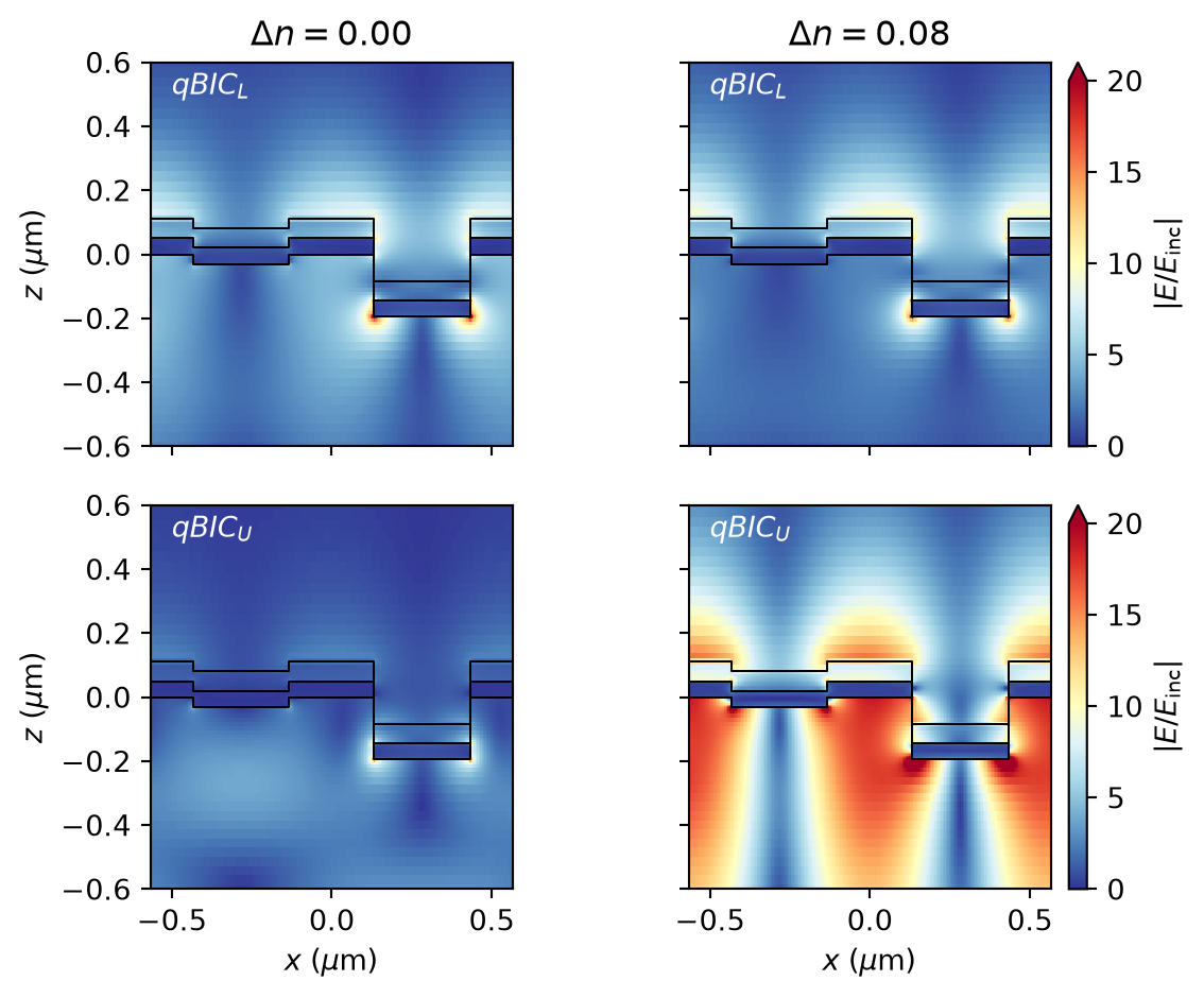
No matching results found.


 TERMS & CONDITIONS


 How the process works:
 Try this real URL to see an example: