Author: Dun Wang, University of Pennsylvania
This notebook demonstrates the calculation of the band structure of hexagonal crystals of air holes in a SiN slab on SiO₂ depending on the topological invariant of the bandgap.
Namely, hole positions are displaced sinusoidally along $x$ by
$$\delta x = dt·\sin(Gₛ·x) + dtt·\sin(2Gₛ·x),$$
where here $G_s$ ≈ 0.925$G_k$, and $G_k=\frac{4\pi}{3a}$, and the coefficients are parameters that control the topological invariant of the gap. Here we reverse the sign of $dtt$ across a domain wall at $x = 0$ to produce a Jackiw–Rebbi interface mode localized at the junction.

# standard python imports
import numpy as np
import matplotlib.pyplot as plt
import xarray as xr

import tidy3d as td
from tidy3d import web
from tidy3d.plugins.resonance import ResonanceFinder
from tidy3d.plugins.dispersion import AdvancedFastFitterParam, FastDispersionFitter
from scipy.optimize import root_scalar
rng = np.random.default_rng(1290)
td.set_logging_level = "ERROR"
Set Up Simulation
a=0.265
H=0.12
d=0.1
W=0.08 #width of square hol
h_space=1
h_top=0.4
h_si=0.4
h_sub=h_space-h_si
dt=0.02
dtt=-0.01

G_K=4*np.pi/(3*a)
G_s=0.925*G_K


theta=0
phi=0

wls=np.linspace(0.6,0.7,1000)  #wavelength range
freqs=td.C_0/wls
freq0=(freqs[0]+freqs[-1])/2
wl0=td.C_0/freq0
fwidth=freqs[0]-freqs[-1]
pulse_width=fwidth
run_time=600/pulse_width

n_air=1
n_medium=2.02
n_bg=1.46
n_Si=3.88
SiN=td.Medium(permittivity=n_medium**2)
SiO2=td.Medium(permittivity=n_bg**2)
Air=td.Medium(permittivity=n_air**2)
Si=td.Medium(permittivity=n_Si**2)

N=30  # 2N = number of unit cells along x
dx=0 # extra space left at x boundary
sim_size=((2*N)*a+2*dx, np.sqrt(3)*a, 2*h_space+H)
slab1 = td.Structure(
    geometry=td.Box(
        center=(0, 0, 0),
        size=(td.inf, td.inf, H),
    ),
    medium=SiN,
    name="slab1",
)

sub_sio2 = td.Structure(
    geometry=td.Box(
        center=(0, 0, -H/2-h_sub/2),
        size=(td.inf, td.inf, h_sub),
    ),
    medium=SiO2,
    name="sub",
)

sub_si=td.Structure(
    geometry=td.Box(
        center=(0, 0, -H/2-h_space),
        size=(td.inf, td.inf, 2*h_si)
    ),
    medium=SiO2,
    name="sub_si",
)

top = td.Structure(
    geometry=td.Box(
        center=(0, 0, H/2+h_top/2),
        size=(td.inf, td.inf, h_top),
    ),
    medium=Air,
    name="top",
)

layers=[top, slab1, sub_sio2,sub_si]

def hex_holes_alongx(a, d, N, G_s, dt):
    holes=[]
    A1=np.array([0, a/np.sqrt(3), 0])
    A2=np.array([-a/2, a/2/np.sqrt(3), 0])
    A3=np.array([-a/2, -a/2/np.sqrt(3), 0])
    A4=np.array([0, -a/np.sqrt(3),0])
    for i in np.arange(-N, N+1):
        r1=np.array([i*a,0,0])+A1
        holes.append(
            td.Cylinder(
                radius=d/2,
                center=tuple(r1 + np.array([dt*np.sin(G_s*r1[0]),0,0]) + np.array([dtt*np.sin(2*G_s*r1[0]),0,0])),
                length=H,
                axis=2
            )
        )
        r2=np.array([i*a,0,0])+A2
        holes.append(
            td.Cylinder(
                radius=d/2,
                center=tuple(r2 + np.array([dt*np.sin(G_s*r2[0]),0,0])+ np.array([dtt*np.sin(2*G_s*r2[0]),0,0])),
                length=H,
                axis=2
            )
        )
        r3=np.array([i*a,0,0])+A3
        holes.append(
            td.Cylinder(
                radius=d/2,
                center=tuple(r3 + np.array([dt*np.sin(G_s*r3[0]),0,0])+ np.array([dtt*np.sin(2*G_s*r3[0]),0,0])),
                length=H,
                axis=2
            )
        )
        r4=np.array([i*a,0,0])+A4
        holes.append(
            td.Cylinder(
                radius=d/2,
                center=tuple(r4 + np.array([dt*np.sin(G_s*r4[0]),0,0])+ np.array([dtt*np.sin(2*G_s*r4[0]),0,0])),
                length=H,
                axis=2
            )
        )
        holes.append(
            td.Cylinder(
                radius=d/2,
                center=tuple(np.array([N*a+a/2, a/2/np.sqrt(3),0]) + np.array([dt*np.sin(G_s*(N*a+a/2)),0,0])+ np.array([dtt*np.sin(2*G_s*(N*a+a/2)),0,0])),
                length=H,
                axis=2
            )
        )
        holes.append(
            td.Cylinder(
                radius=d/2,
                center=tuple(np.array([N*a+a/2, -a/2/np.sqrt(3),0]) + np.array([dt*np.sin(G_s*(N*a+a/2)),0,0])+ np.array([dtt*np.sin(2*G_s*(N*a+a/2)),0,0])),
                length=H,
                axis=2
            )
        )
    holes_geo = td.GeometryGroup(geometries=holes)
    return [td.Structure(geometry=holes_geo, medium=Air, name="holes")]

structures=layers+hex_holes_alongx(a,d,N,G_s, dt)
def circular_source(pol, theta, phi):
    # define a circularly polarized plane wave incident at angle theta phi
    plane_wave_x = td.PlaneWave(
        source_time=td.GaussianPulse(freq0=freq0, fwidth=pulse_width),
        size=(td.inf, td.inf, 0),
        center=(0, 0, 0.5*H+0.7*h_space),
        direction="-",
        angle_theta=theta,
        angle_phi=phi,
        pol_angle=np.pi/2,
    )

    # determine the phase difference given the polarization
    if pol == "LCP":
        phase = -np.pi / 2
    elif pol == "RCP":
        phase = np.pi / 2
    else:
        raise ValueError("pol must be `LCP` or `RCP`")

    # define a plane wave polarized in the y direction with a phase difference
    plane_wave_y = td.PlaneWave(
        source_time=td.GaussianPulse(freq0=freq0, fwidth=pulse_width, phase=phase),
        size=(td.inf, td.inf, 0),
        center=(0, 0, 0.5*H+0.7*h_space),
        direction="-",
        angle_theta=theta,
        angle_phi=phi,
        pol_angle=np.pi / 2-phi,
    )

    return [plane_wave_y]

monitor_r = td.FluxMonitor(
    center=[0, 0, 0.5*H+0.9*h_space], size=[td.inf, td.inf, 0], freqs=freqs, name="R"
)
monitor_t = td.FluxMonitor(
    center=[0, 0, -0.5*H-0.9*h_space], size=[td.inf, td.inf, 0], freqs=freqs, name="T"
)

def makesim(pol:str, theta:float, phi:float, dt:float, j:int):
    source=circular_source(pol, theta, phi)

    # Bloch boundaries from source.
    bloch_x = td.Boundary.bloch_from_source(
          source=source[0],
          domain_size=sim_size[0],
          axis=0,
          medium=Air
    )

    bloch_y = td.Boundary.bloch_from_source(
          source=source[0],
          domain_size=sim_size[1],
          axis=1,
          medium=Air
    )

    num_pml=30

    bspecs = td.BoundarySpec(x=bloch_x, y=bloch_y, z=td.Boundary.pml())


    refine_box = td.MeshOverrideStructure(
    geometry=td.Box(center=(0, 0, 0), size=(td.inf, td.inf, H)),
    dl=[0.04, 0.04, 0.02],
    )


    sim = td.Simulation(
            size=sim_size,
            center=(0, 0, 0),
            grid_spec=td.GridSpec.auto(min_steps_per_wvl=8, wavelength=wl0),
            structures=structures,
            medium=Air,
            sources=source,
            monitors=[monitor_r],
            run_time=run_time,
            boundary_spec=bspecs,
            shutoff=1e-5,
        )
    return sim
sims={}
N_angle=20
angle_max=15*np.pi/180 ##NA=0.25
k_max=1/wl0*np.sin(angle_max)
for i in range(N_angle):
    k_i=0+k_max*i/N_angle
    theta=np.arcsin(k_i*wl0)
    phi=np.pi/2
    sims[f"sim_{i}"] = makesim("LCP", theta, phi, dt,i)
sims["sim_0"].plot_3d()
plt.show()
sims["sim_19"].plot_3d()
plt.show()
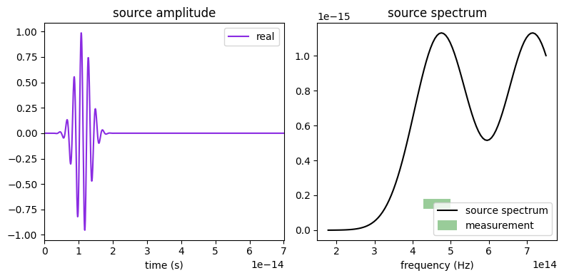
f, (ax1, ax2) = plt.subplots(1, 2, tight_layout=True, figsize=(8, 4))
plot_time = 5 / fwidth
ax1 = (
    sims["sim_0"]
    .sources[0]
    .source_time.plot(times=np.linspace(0, plot_time, 1001), val="real", ax=ax1)
)
ax1.set_xlim(0, plot_time)
ax2 = (
    sims["sim_0"]
    .sources[0]
    .source_time.plot_spectrum(
        times=np.linspace(0, sims["sim_0"].run_time, 10001), val="abs", ax=ax2
    )
)
ax2.hlines(1.5e-16, freqs[-1], freqs[0], linewidth=10, color="g", alpha=0.4)
ax2.legend(("source spectrum", "measurement"))
plt.show()
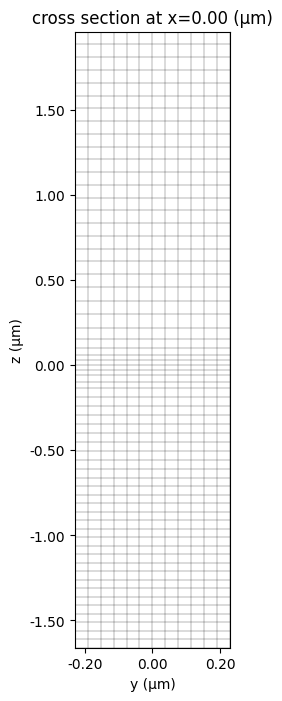
fig, ax=plt.subplots(1,1, figsize=(2,8))
sims["sim_0"].plot_grid(x=0, ax=ax)
#ax.set_ylim(-sim_size[2]/2,sim_size[2]/2)
<Axes: title={'center': 'cross section at x=0.00 (μm)'}, xlabel='y (μm)', ylabel='z (μm)'>
Run
# job = web.Job(simulation=sims["sim_1"], task_name="job", verbose="True")
# # # estimate the maximum cost
# estimated_cost = web.estimate_cost(job.task_id)

batch = web.Batch(simulations=sims, folder_name='data', verbose=True)
batch_data = batch.run(path_dir='data')
Output()
08:31:09 EDT Started working on Batch containing 20 tasks.
08:31:38 EDT Maximum FlexCredit cost: 1.154 for the whole batch.
             Use 'Batch.real_cost()' to get the billed FlexCredit cost after the
             Batch has completed.
Output()
08:31:55 EDT Batch complete.
Output()
flux_sig = np.zeros((0, len(freqs)))
for i in range(N_angle):
    flux_sig = np.vstack((flux_sig, batch_data[f"sim_{i}"].monitor_data['R'].flux.squeeze()))
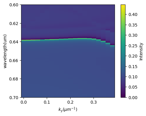
Band Structure
flux_now=flux_sig

# N_angle=16
# wls=np.linspace(0.585,0.685,2000)
# freqs=td.C_0/wls
K, F = np.meshgrid((np.sin(angle_max*np.arange(N_angle)/N_angle))/wl0, td.C_0/freqs)
flux_plot=flux_now
plt.figure(figsize=(5,4))
plt.pcolormesh(K.T, F.T, flux_plot, shading='nearest' , cmap='viridis', vmin=0)
plt.colorbar(label="Intensity")

plt.rcParams['text.usetex'] = True
plt.xlabel("$k_y (\mu m^{-1})$")
plt.ylabel("wavelength(um)")
#plt.xlim(0, 0.04)
#plt.ylim(0.62, 0.66)
plt.gca().invert_yaxis()
plt.show()
plt.rcParams['text.usetex'] = False
#np.savetxt('R_RCP_h=130nm_dt=30_y.txt', flux_sig)
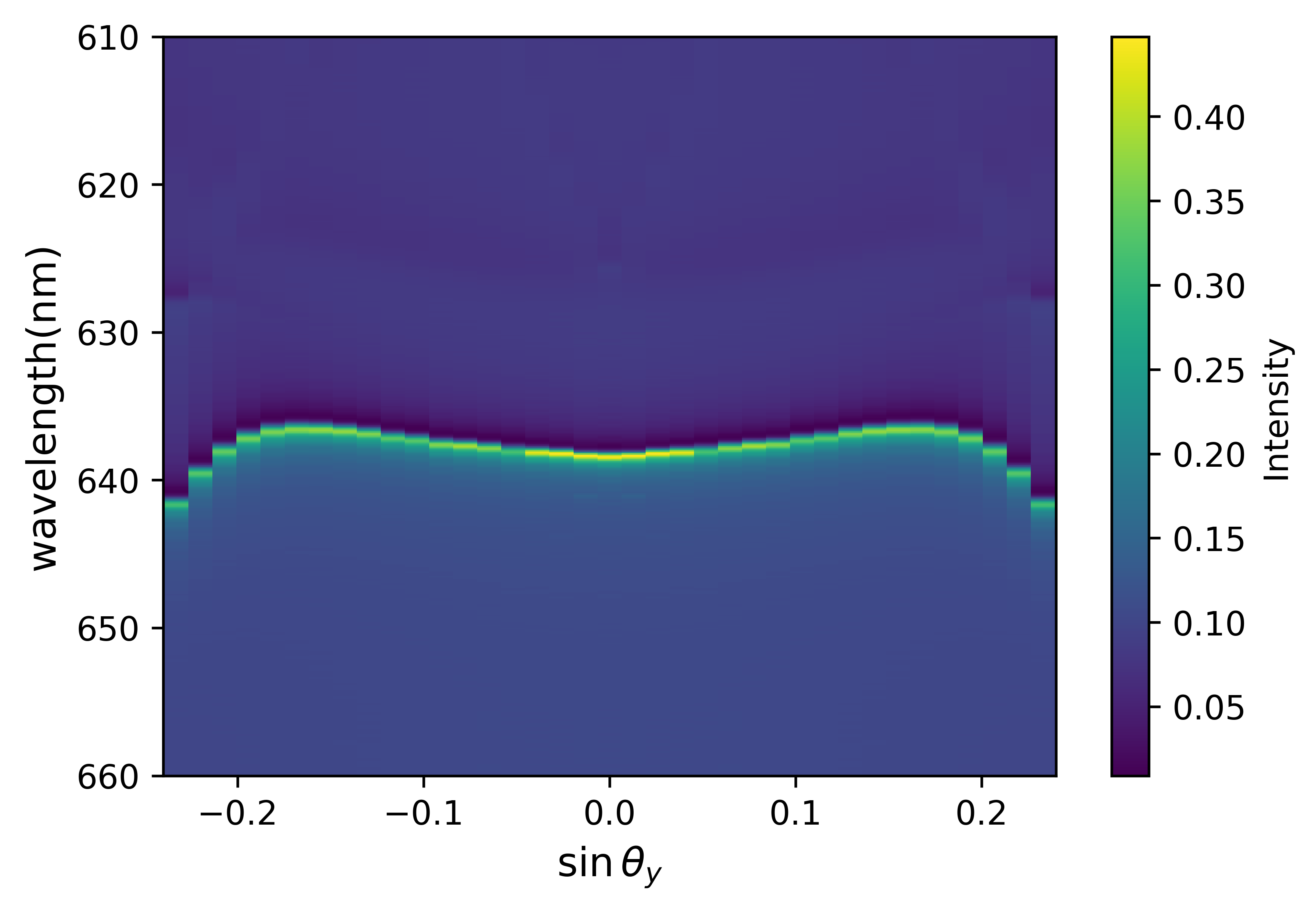
flux_plot = np.vstack((np.flipud(flux_now)[0:-1, :], flux_now))
# wls=np.linspace(0.567,0.667,1000)
# freqs=td.C_0/wls
# angle_max=20*np.pi/180
K, F = np.meshgrid(np.sin(angle_max)*np.arange(-N_angle+1,N_angle)/N_angle, td.C_0/freqs*1000)
plt.figure(figsize=(6,4), dpi=600)
plt.pcolormesh(K.T, F.T, flux_plot, shading='nearest' , cmap='viridis')
plt.colorbar(label="Intensity")

# plt.rcParams.update({'font.size': 12})          # Default text size
# plt.rcParams.update({'axes.titlesize': 16})     # Title size
# plt.rcParams.update({'axes.labelsize': 10})     # X and Y label size
plt.rcParams.update({'xtick.labelsize': 10})    # X-tick size
plt.rcParams.update({'ytick.labelsize': 10})    # X-tick size
# plt.rcParams.update({'legend.fontsize': 10})    # Legend size

plt.rcParams['text.usetex'] = True
plt.xlabel(r"$\sin \theta_y$", fontsize=12)
plt.ylabel("wavelength(nm)", fontsize=12)
plt.xlim(-0.24, 0.24)
plt.ylim((610,660))

plt.gca().invert_yaxis()

plt.show()
plt.rcParams['text.usetex'] = False
#np.savetxt('R_RCP_h=130nm_dt=30_y.txt', flux_sig)
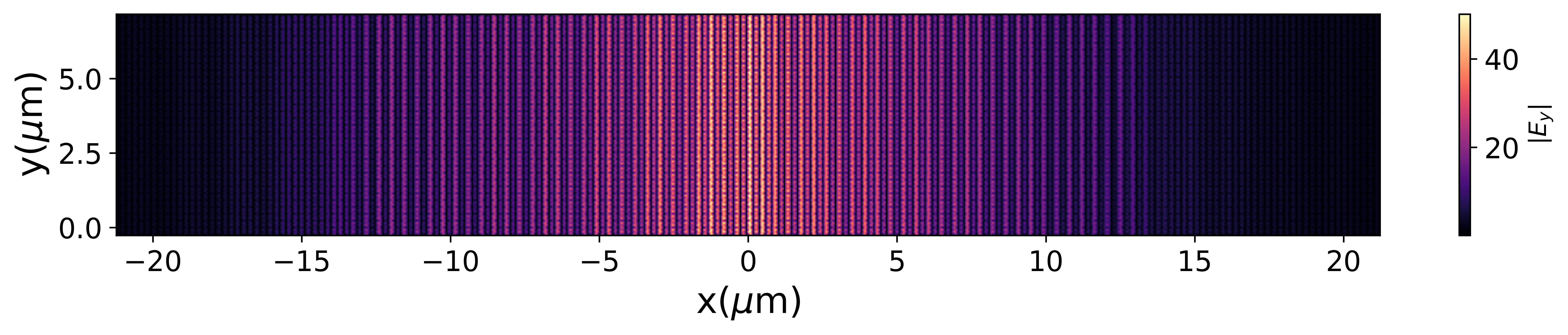
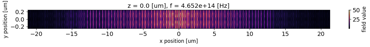
Jackiw-Rebbi Interface State
The sign of dtt is flipped between the left (x < 0) and right (x > 0) halves of the structure. The two halves are topologically distinct, and a spatially localized in-gap mode forms at the domain wall.
Set Up Simulation
a=0.265
H=0.12
d=0.1

h_space=1.2
h_top=0.4
h_si=0.4
h_sub=h_space-h_si
dt=0.02
dtt=0.01

G_K=4*np.pi/(3*a)
G_s=0.925*G_K


theta=0
phi=0

wls=np.linspace(0.6,0.7,1000)  #wavelength range
freqs=td.C_0/wls
freq0=(freqs[0]+freqs[-1])/2
wl0=td.C_0/freq0
fwidth=freqs[0]-freqs[-1]
pulse_width=fwidth
run_time=800/pulse_width

n_air=1
n_medium=2.02
n_bg=1.46
n_Si=3.88
SiN=td.Medium(permittivity=n_medium**2)
SiO2=td.Medium(permittivity=n_bg**2)
Air=td.Medium(permittivity=n_air**2)
Si=td.Medium(permittivity=n_Si**2)

N=100  # 2N+1 = number of unit cells along x
dx=1 # extra space left at x boundary
sim_size=((2*N+1)*a+2*dx, np.sqrt(3)*a, 2*h_space+H)
slab1 = td.Structure(
    geometry=td.Box(
        center=(0, 0, 0),
        size=(td.inf, td.inf, H),
    ),
    medium=SiN,
    name="slab1",
)

sub_sio2 = td.Structure(
    geometry=td.Box(
        center=(0, 0, -H/2-h_sub/2),
        size=(td.inf, td.inf, h_sub),
    ),
    medium=SiO2,
    name="sub",
)

sub_si=td.Structure(
    geometry=td.Box(
        center=(0, 0, -H/2-h_space),
        size=(td.inf, td.inf, 2*h_si)
    ),
    medium=SiO2,
    name="sub_si",
)

top = td.Structure(
    geometry=td.Box(
        center=(0, 0, H/2+h_top/2),
        size=(td.inf, td.inf, h_top),
    ),
    medium=Air,
    name="top",
)

# monolayer = td.Structure(
#     geometry=td.Box(
#         center=(0, 0, H/2+t_MoS2/2),
#         size=(td.inf, td.inf, t_MoS2),
#     ),
#     medium=MoS2,      #td.material_library['MoS2']['Li2014'],
#     name="monolayer",
# )

layers=[top, slab1, sub_sio2,sub_si]

def hex_holes_alongx_JR(a, d, N, G_s, dt, dtt):
    holes=[]
    A1=np.array([0, a/np.sqrt(3), 0])
    A2=np.array([-a/2, a/2/np.sqrt(3), 0])
    A3=np.array([-a/2, -a/2/np.sqrt(3), 0])
    A4=np.array([0, -a/np.sqrt(3),0])
    for i in np.arange(-N, 1):
        r1=np.array([-i*a,0,0])+A1
        holes.append(
            td.Cylinder(
                radius=d/2,
                center=tuple(r1 + np.array([dt*np.sin(G_s*r1[0]),0,0]) + np.array([dtt*np.sin(2*G_s*r1[0]),0,0])),
                length=H,
                axis=2
            )
        )
        r2=np.array([-i*a,0,0])+A2
        holes.append(
            td.Cylinder(
                radius=d/2,
                center=tuple(r2 + np.array([dt*np.sin(G_s*r2[0]),0,0])+ np.array([dtt*np.sin(2*G_s*r2[0]),0,0])),
                length=H,
                axis=2
            )
        )
        r3=np.array([-i*a,0,0])+A3
        holes.append(
            td.Cylinder(
                radius=d/2,
                center=tuple(r3 + np.array([dt*np.sin(G_s*r3[0]),0,0])+ np.array([dtt*np.sin(2*G_s*r3[0]),0,0])),
                length=H,
                axis=2
            )
        )
        r4=np.array([-i*a,0,0])+A4
        holes.append(
            td.Cylinder(
                radius=d/2,
                center=tuple(r4 + np.array([dt*np.sin(G_s*r4[0]),0,0])+ np.array([dtt*np.sin(2*G_s*r4[0]),0,0])),
                length=H,
                axis=2
            )
        )
    dtt=-dtt
    for i in np.arange(1, N+1):
        r1=np.array([-i*a,0,0])+A1
        holes.append(
            td.Cylinder(
                radius=d/2,
                center=tuple(r1 + np.array([dt*np.sin(G_s*r1[0]),0,0]) + np.array([dtt*np.sin(2*G_s*r1[0]),0,0])),
                length=H,
                axis=2
            )
        )
        r2=np.array([-i*a,0,0])+A2
        holes.append(
            td.Cylinder(
                radius=d/2,
                center=tuple(r2 + np.array([dt*np.sin(G_s*r2[0]),0,0])+ np.array([dtt*np.sin(2*G_s*r2[0]),0,0])),
                length=H,
                axis=2
            )
        )
        r3=np.array([-i*a,0,0])+A3
        holes.append(
            td.Cylinder(
                radius=d/2,
                center=tuple(r3 + np.array([dt*np.sin(G_s*r3[0]),0,0])+ np.array([dtt*np.sin(2*G_s*r3[0]),0,0])),
                length=H,
                axis=2
            )
        )
        r4=np.array([-i*a,0,0])+A4
        holes.append(
            td.Cylinder(
                radius=d/2,
                center=tuple(r4 + np.array([dt*np.sin(G_s*r4[0]),0,0])+ np.array([dtt*np.sin(2*G_s*r4[0]),0,0])),
                length=H,
                axis=2
            )
        )
    holes.append(
        td.Cylinder(
            radius=d/2,
            center=tuple(np.array([N*a+a/2, a/2/np.sqrt(3),0]) + np.array([dt*np.sin(G_s*(N*a+a/2)),0,0])+ np.array([dtt*np.sin(2*G_s*(N*a+a/2)),0,0])),
            length=H,
            axis=2
        )
    )
    holes.append(
        td.Cylinder(
            radius=d/2,
            center=tuple(np.array([N*a+a/2, -a/2/np.sqrt(3),0]) + np.array([dt*np.sin(G_s*(N*a+a/2)),0,0])+ np.array([dtt*np.sin(2*G_s*(N*a+a/2)),0,0])),
            length=H,
            axis=2
        )
    )
    holes_geo = td.GeometryGroup(geometries=holes)
    return [td.Structure(geometry=holes_geo, medium=Air, name="holes")]


structures=layers+hex_holes_alongx_JR(a,d,N,G_s, dt, dtt)
def finite_source(pol, theta, phi, S):
    # define a circularly polarized plane wave incident at angle theta phi
    plane_wave_x = td.PlaneWave(
        source_time=td.GaussianPulse(freq0=freq0, fwidth=pulse_width),
        size=(S, td.inf, 0),
        center=(0, 0, 0.5*H+0.7*h_space),
        direction="-",
        angle_theta=theta,
        angle_phi=phi,
        pol_angle=0,
    )

    # determine the phase difference given the polarization
    if pol == "LCP":
        phase = -np.pi / 2
    elif pol == "RCP":
        phase = np.pi / 2
    else:
        raise ValueError("pol must be `LCP` or `RCP`")

    # define a plane wave polarized in the y direction with a phase difference
    plane_wave_y = td.PlaneWave(
        source_time=td.GaussianPulse(freq0=freq0, fwidth=pulse_width, phase=phase),
        size=(S, td.inf, 0),
        center=(0, 0, 0.5*H+0.7*h_space),
        direction="-",
        angle_theta=theta,
        angle_phi=phi,
        pol_angle=np.pi / 2-phi,
    )

    return [plane_wave_y]

monitor_r = td.FluxMonitor(
    center=[0, 0, 0.5*H+0.9*h_space], size=[td.inf, td.inf, 0], freqs=freqs, name="R"
)
monitor_t = td.FluxMonitor(
    center=[0, 0, -0.5*H-0.9*h_space], size=[td.inf, td.inf, 0], freqs=freqs, name="T"
)

monitor_fz=td.FieldMonitor(
    center=[0,0,0], size=[160*a, sim_size[1], 0], freqs=freqs, name="fz"
)

def makesim_JR(pol:str, theta:float, phi:float, S:float, j:int):
    source=finite_source(pol, theta, phi, S)

    # Bloch boundaries from source.
    bloch_x = td.Boundary.bloch_from_source(
          source=source[0],
          domain_size=sim_size[0],
          axis=0,
          medium=Air
    )

    bloch_y = td.Boundary.bloch_from_source(
          source=source[0],
          domain_size=sim_size[1],
          axis=1,
          medium=Air
    )

    num_pml=30

    bspecs = td.BoundarySpec(x=bloch_x, y=bloch_y, z=td.Boundary.pml())

    # refine_box = td.MeshOverrideStructure(
    # geometry=td.Box(center=(0, 0, -H/2-(h_sub+h_space)/2), size=(td.inf, td.inf, h_space-h_sub)),
    # dl=[0.04, 0.04, 0.08],
    # )


    sim = td.Simulation(
            size=sim_size,
            center=(0, 0, 0),
            grid_spec=td.GridSpec.auto(min_steps_per_wvl=8, wavelength=wl0),
            structures=structures,
            medium=Air,
            sources=source,
            monitors=[monitor_r, monitor_fz],
            run_time=run_time,
            boundary_spec=bspecs,
#             boundary_spec=td.BoundarySpec(
#                 x=td.Boundary.periodic(), y=td.Boundary.periodic(), z=td.Boundary.pml()
#             ),
            shutoff=1e-5,
        )
    return sim
sims={}
N_angle=1
angle_max=15*np.pi/180
S=100*a
k_max=1/wl0*np.sin(angle_max)
for i in range(N_angle):
k_i=0+k_max*i/N_angle
theta=np.arcsin(k_i*wl0)
phi=0
sims[f"sim_{i}"] = makesim_JR("RCP", theta, phi, S, i)
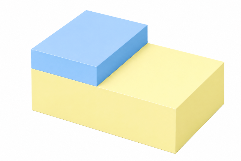
sims["sim_0"].plot_3d()
plt.show()
job = web.Job(simulation=sims["sim_0"], task_name="job", verbose="True")
# # estimate the maximum cost
estimated_cost = web.estimate_cost(job.task_id)

# batch = web.Batch(simulations=sims, folder_name='data', verbose=True)
# batch_data = batch.run(path_dir='data')
08:32:21 EDT Created task 'job' with task_id
             'fdve-1c1fe08d-d2e0-4f3e-83c1-742202508d54' and task_type 'FDTD'.
             View task using web UI at
             'https://tidy3d.simulation.cloud/workbench?taskId=fdve-1c1fe08d-d2e
             0-4f3e-83c1-742202508d54'.
Task folder: 'default'.
Output()
08:32:29 EDT Maximum FlexCredit cost: 0.385. Minimum cost depends on task
             execution details. Use 'web.real_cost(task_id)' to get the billed
             FlexCredit cost after a simulation run.
08:32:33 EDT Maximum FlexCredit cost: 0.385. Minimum cost depends on task
             execution details. Use 'web.real_cost(task_id)' to get the billed
             FlexCredit cost after a simulation run.
flux_sig=flux_now
flux_sig.shape
(20, 1000)
Run
results = job.run()
# flux_sig = np.zeros((0, len(freqs)))
# for i in range(N_angle):
#     flux_sig = np.vstack((flux_sig, batch_data[f"sim_{i}"].monitor_data['R'].flux.squeeze()))
08:32:36 EDT status = queued
             To cancel the simulation, use 'web.abort(task_id)' or
             'web.delete(task_id)' or abort/delete the task in the web UI.
             Terminating the Python script will not stop the job running on the
             cloud.
Output()
08:32:45 EDT status = preprocess
08:32:50 EDT starting up solver
running solver
Output()
08:34:37 EDT early shutoff detected at 24%, exiting.
08:34:47 EDT status = success
             View simulation result at
             'https://tidy3d.simulation.cloud/workbench?taskId=fdve-1c1fe08d-d2e
             0-4f3e-83c1-742202508d54'.
Output()
08:44:13 EDT loading simulation from simulation_data.hdf5
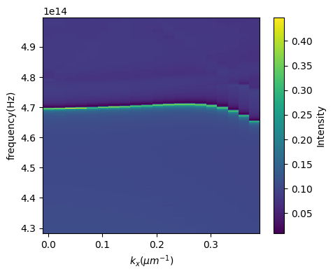
#angle_max=15
N_plot = flux_now.shape[0]
K, F = np.meshgrid((np.sin(angle_max*np.arange(N_plot)/N_plot))/wl0, freqs)
flux_plot=flux_now
# mask1 = flux_plot<0
# flux_plot[mask1] = 0
# mask2 = flux_plot>1
# flux_plot[mask2] = 1
plt.figure(figsize=(5,4))
plt.pcolormesh(K.T, F.T, flux_plot, shading='nearest' , cmap='viridis')
plt.colorbar(label="Intensity")

plt.rcParams['text.usetex'] = True
plt.xlabel("$k_x (\mu m^{-1})$")
plt.ylabel("frequency(Hz)")
#plt.xlim(0, 0.04)
#plt.ylim(4.4e14, 4.8e14)

plt.show()
plt.rcParams['text.usetex'] = False
#np.savetxt('R_RCP_h=130nm_dt=30_y.txt', flux_sig)
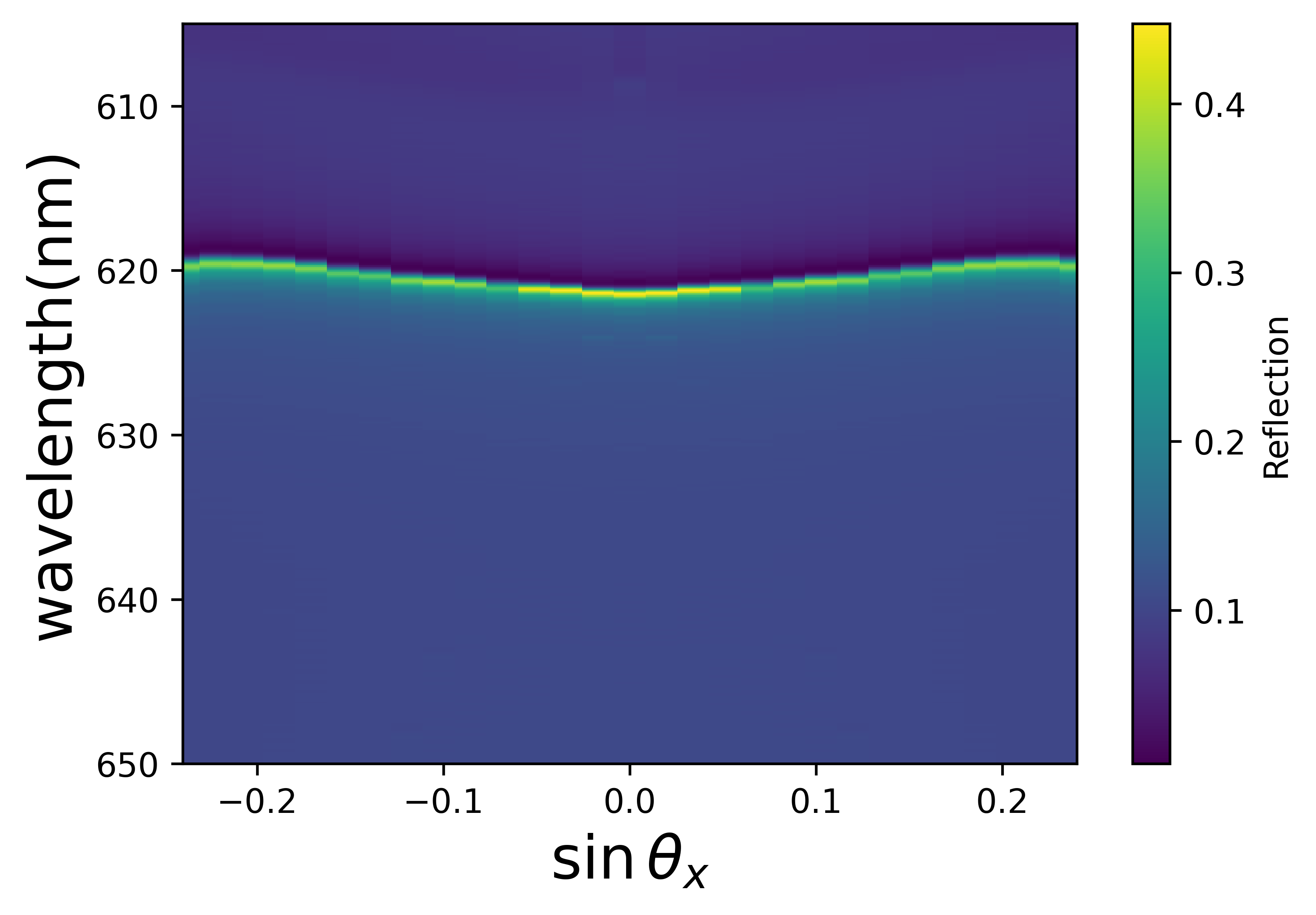
flux_plot = np.vstack((np.flipud(flux_now)[0:-1, :], flux_now))
wls=np.linspace(0.583,0.683,1000)
freqs=td.C_0/wls
angle_max=20*np.pi/180
N_angle = flux_now.shape[0]
K, F = np.meshgrid(np.sin(angle_max)*np.arange(-N_angle+1,N_angle)/N_angle, td.C_0/freqs*1000)
plt.figure(figsize=(6,4), dpi=600)
plt.pcolormesh(K.T, F.T, flux_plot, shading='nearest' , cmap='viridis')
plt.colorbar(label="Reflection")

plt.rcParams.update({'font.size': 12})          # Default text size
# plt.rcParams.update({'axes.titlesize': 16})     # Title size
# plt.rcParams.update({'axes.labelsize': 10})     # X and Y label size
plt.rcParams.update({'xtick.labelsize': 14})    # X-tick size
plt.rcParams.update({'ytick.labelsize': 14})    # Y-tick size
# plt.rcParams.update({'legend.fontsize': 10})    # Legend size

plt.rcParams['text.usetex'] = True
plt.xlabel(r"$\sin \theta_x$", fontsize=18)
plt.ylabel("wavelength(nm)", fontsize=18)
plt.xlim(-0.24, 0.24)
plt.ylim((605,650))

plt.gca().invert_yaxis()

plt.show()
plt.rcParams['text.usetex'] = False
#np.savetxt('R_RCP_h=130nm_dt=30_y.txt', flux_sig)
Results
RR=results.monitor_data["R"].flux
plt.plot(freqs, RR)
#plt.xlim([4.6e14,4.8e14])
[<matplotlib.lines.Line2D at 0x133efc100>]
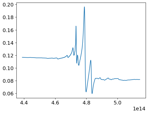
frange = (freqs > 4.65e14) & (freqs < 4.7e14)
index_peak = np.argmin(np.array(RR[frange]))
f_peak=freqs[frange][index_peak]
# results.plot_field(
#     field_monitor_name="fz",
#     field_name="Ey",
#     val="abs",
#     f=f_peak,
#     eps_alpha=0.2,
# )
field_Ey = results.monitor_data["fz"].Ey.interp(f=float(f_peak))
field_Ey.squeeze()
field_Ey.abs.plot(x="x", y="y", figsize=(16, 0.8), cmap="magma")
<matplotlib.collections.QuadMesh at 0x130dc6490>
field=field_Ey.values
field=field[:,:,0]
x_vals = field_Ey.coords['x'].values
y_vals = field_Ey.coords['y'].values
field.shape
(1062, 13)
Num=16
field_stacked=np.tile(field, (1,Num))
y_step=sim_size[1]
y_stack=y_vals
for i in range(Num-1):
    y_stack=np.concatenate([y_stack, y_vals+(i+1)*y_step], axis=0)
X,Y = np.meshgrid(x_vals, y_stack)
plt.figure(figsize=(14.2,2), dpi=600)
plt.pcolormesh(X.T,Y.T,np.abs(field_stacked), shading="nearest", cmap="magma" )
plt.colorbar(label="$|E_y|$")
plt.rcParams.update({'font.size': 12})          # Default text size
plt.rcParams.update({'xtick.labelsize': 14})    # X-tick size
plt.rcParams.update({'ytick.labelsize': 14})    # Y-tick size
plt.xlabel("x($\mu$m)", fontsize=18)
plt.ylabel("y($\mu$m)", fontsize=18)
plt.xlim(np.min(x_vals), np.max(x_vals))
plt.ylim(np.min(y_stack), np.max(y_stack))
plt.axis("equal")
plt.margins(x=0)
plt.margins(y=0)
plt.show()