Author: Tianle Xu, Rensselaer Polytechnic Institute (RPI)
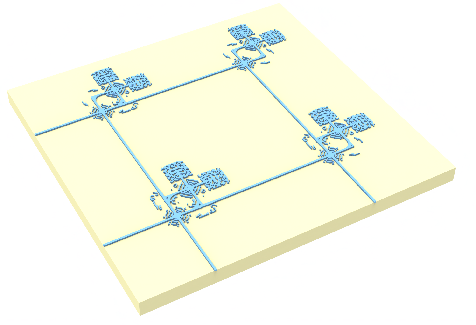
This example demonstrates the co-optimization of two separate design regions using Tidy3D inverse design with native automatic differentiation support. In this framework, regular Tidy3D components and web.run() functions are differentiable without any change of syntax.
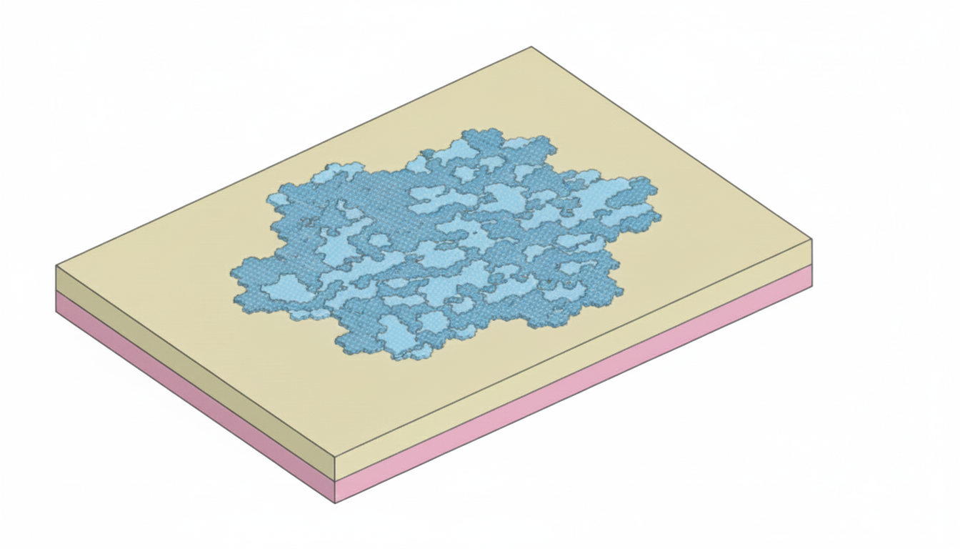
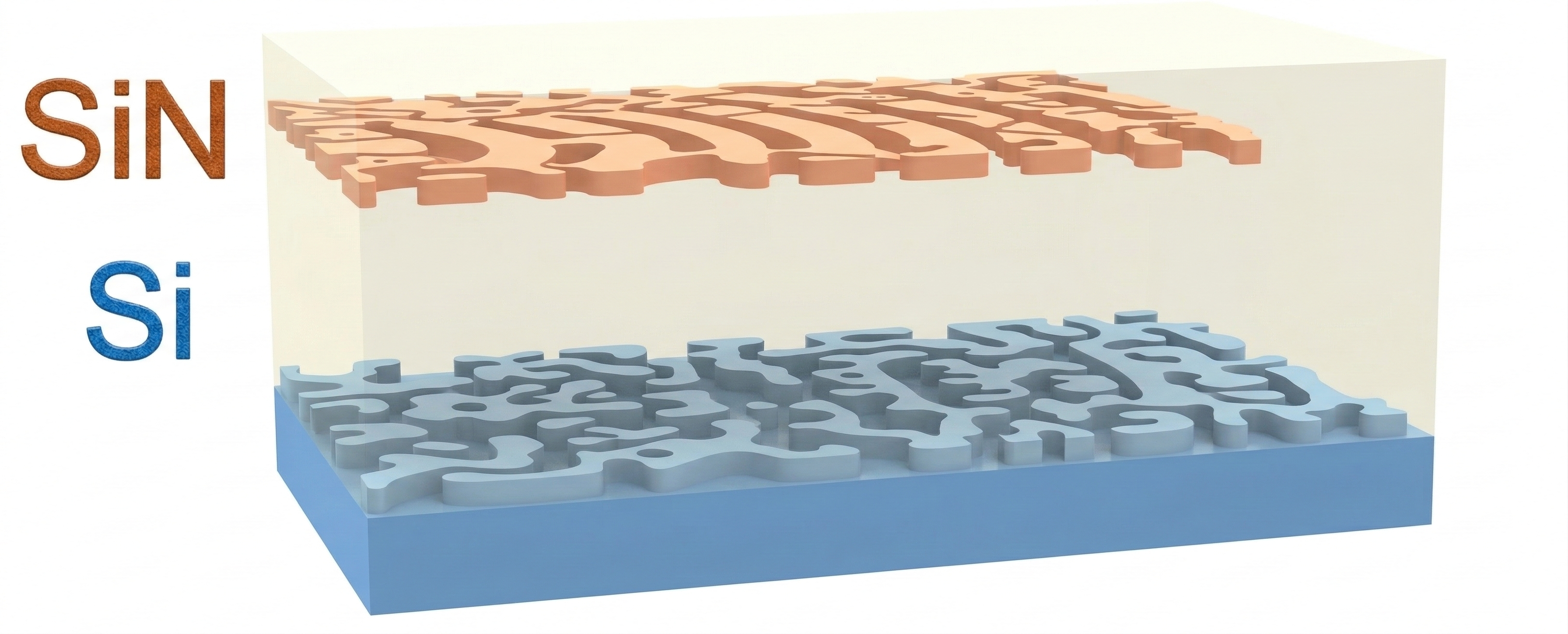
We optimize a grating coupler for coupling efficiency with respect to
- the pattern partially etched into a Si coupling layer.
- the pattern etched into a SiN layer suspended above the coupling region.
Our example roughly follows the paper Thomas Van Vaerenbergh, Sean Hooten, Mudit Jain, Peng Sun, Quentin Wilmart, Ashkan Seyedi, Zhihong Huang, Marco Fiorentino, and Ray Beausoleil, "Wafer-level testing of inverse-designed and adjoint-inspired dual layer Si-SiN vertical grating couplers", Journal of Physics: Photonics 4(4), (2022). DOI: https://doi.org/10.1088/2515-7647/ac943c paper.
import autograd
import autograd.numpy as np
import matplotlib.pylab as plt
import tidy3d as td
import tidy3d.web as web

# define some length scales in Tidy3D default of microns
um = 1.0
nm = 1e-3
17:11:38 -03 WARNING: Using canonical configuration directory at
             '/home/filipe/.config/tidy3d'. Found legacy directory at
             '~/.tidy3d', which will be ignored. Remove it manually or run
             'tidy3d config migrate --delete-legacy' to clean up.
Set up Simulation
First, we define everything "static" (not optimizing) in the simulation, including parameters and Tidy3D components.
Spectral Parameters
wavelength = 1550 * nm
freq = td.C_0 / wavelength
fwidth = freq / 10
run_time = 50 / fwidth
Geometric Parameters
All the thicknesses are according to the AIM photonic PDK.
The design size follows the work from IMEC, where the BCB to SiN layer difference is 50 nm. This can be ignored.
# device parameters
thick_substrate = 2.0 * um
thick_Si = 220 * nm
thick_SiN = 220 * nm
thick_etch = 220 * nm
space_SiSiN = 100 * nm
width_waveguide = 1000 * nm

# size of design region
size_design_x = 8 * um
size_design_y = 8 * um

# spacings between things (technically infinite, but finite for sim)
length_waveguide = 1 * wavelength
thick_Si_substrate = 550 * nm
space_cladding_top = 1 * wavelength
space_design_edge = 1 * wavelength

# compute sim size
size_sim_x = length_waveguide + size_design_x + space_design_edge
size_sim_y = space_design_edge + size_design_y + space_design_edge
size_sim_z = (
    thick_Si_substrate
    + thick_substrate
    + thick_Si
    + space_SiSiN
    + thick_SiN
    + space_cladding_top
)
size_sim = (size_sim_x, size_sim_y, size_sim_z)

# references to various locations
sim_top_z = size_sim_z / 2.0
sim_bot_z = -size_sim_z / 2.0
center_SiN_z = sim_top_z - space_cladding_top - thick_SiN / 2.0
center_Si_z = sim_top_z - space_cladding_top - thick_SiN - space_SiSiN - thick_Si / 2.0
center_Si_etch_z = (
    sim_top_z - space_cladding_top - thick_SiN - space_SiSiN - thick_etch / 2.0
)
center_source_z = sim_top_z - space_cladding_top / 2.0
center_Si_substrate_z = sim_bot_z + thick_Si_substrate / 2

center_waveguide_x = -size_sim_x / 2 + length_waveguide / 2.0
center_design_x = size_sim_x / 2.0 - space_design_edge - size_design_x / 2.0
Material Parameters
# dispersionless materials for now. Note: can also do `td.Medium.from_nk(n=n, k=k, freq=freq)`

n_SiO2 = 1.44
n_SiN = 2.0
n_Si = 3.5

eps_Si = n_Si**2
eps_SiN = n_SiN**2
eps_SiO2 = n_SiO2**2

medium_Si = td.Medium(permittivity=eps_Si)
medium_SiN = td.Medium(permittivity=eps_SiN)
medium_SiO2 = td.Medium(permittivity=eps_SiO2)
Source Parameters
spot_size = np.sqrt(size_design_x**2 + size_design_y**2)
tilt_angle_deg = 0.0
Static Components
waveguide = td.Structure(
    geometry=td.Box(
        center=(-size_sim_x + length_waveguide + size_design_x / 2.0, 0, center_Si_z),
        size=(size_sim_x, width_waveguide, thick_Si),
    ),
    medium=medium_SiN,
)

design_region = td.Structure(
    geometry=td.Box(
        center=(center_design_x, 0, center_Si_z),
        size=(size_design_x, size_design_y, thick_Si),
    ),
    medium=medium_SiN,
)

slab_SiN = td.Structure(
    geometry=td.Box(
        center=(center_design_x, 0, center_SiN_z),
        size=(size_design_x, size_design_y, thick_SiN),
    ),
    medium=medium_SiN,
)

substrate_Si = td.Structure(
    geometry=td.Box(
        center=(0, 0, -size_sim_z + thick_Si_substrate),
        size=(td.inf, td.inf, size_sim_z),
    ),
    medium=medium_Si,
)

gaussian_beam = td.GaussianBeam(
    center=(center_design_x, 0, center_source_z),
    size=(size_design_x, size_design_y, 0),
    source_time=td.GaussianPulse(freq0=freq, fwidth=fwidth),
    pol_angle=np.pi / 2,
    angle_theta=tilt_angle_deg * np.pi / 180.0,
    direction="-",
    num_freqs=7,
    waist_radius=spot_size / 2,
)

mode_monitor = td.ModeMonitor(
    size=(0, width_waveguide * 6, thick_Si * 6),
    center=(center_waveguide_x, 0, center_Si_z),
    name="mode",
    freqs=[freq],
    mode_spec=td.ModeSpec(),
)

field_monitor_xy = td.FieldMonitor(
    center=(0, 0, center_Si_z),
    size=(td.inf, td.inf, 0),
    freqs=[freq],
    name="field_xy",
)

field_monitor_xz = td.FieldMonitor(
    center=(0, 0, 0),
    size=(td.inf, 0, td.inf),
    freqs=[freq],
    name="field_xz",
)

sim_no_etch = td.Simulation(
    size=size_sim,
    run_time=run_time,
    medium=medium_SiO2,
    structures=[waveguide, design_region, slab_SiN, substrate_Si],
    grid_spec=td.GridSpec.auto(wavelength=wavelength),
    sources=[gaussian_beam],
    monitors=[mode_monitor, field_monitor_xy, field_monitor_xz],
)
# shift the plot positions a little so the field monitors don't overlap plots
shift_plot = 0.01
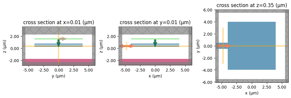
f, (ax1, ax2, ax3) = plt.subplots(1, 3, figsize=(10, 4), tight_layout=True)
sim_no_etch.plot(x=0.0 + shift_plot, ax=ax1)
sim_no_etch.plot(y=0.0 + shift_plot, ax=ax2)
sim_no_etch.plot(z=center_Si_z + shift_plot, ax=ax3)
plt.show()
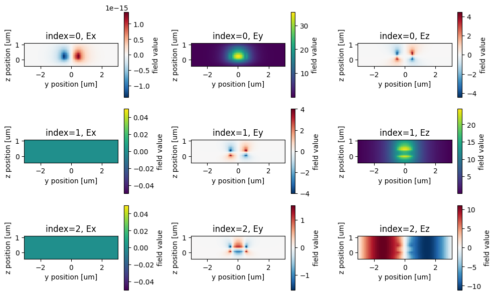
Inspect Waveguide Modes
We will run the mode solver to determine the proper mode_index corresponding to the fundamental TE mode.
from tidy3d.plugins.mode import ModeSolver
from tidy3d.plugins.mode.web import run as run_mode_solver

num_modes = 3
mode_spec = td.ModeSpec(num_modes=num_modes)

mode_solver = ModeSolver(
    simulation=sim_no_etch,
    plane=mode_monitor.geometry,
    mode_spec=mode_spec,
    freqs=[freq],
)
modes = run_mode_solver(mode_solver, reduce_simulation=True)
17:11:43 -03 Mode solver created with
             task_id='fdve-1cb352f3-8a56-4e86-8872-df8cd7bd4e8a',
             solver_id='mo-14d77154-693b-4104-8b42-a83a7cdd46bb'.
Output()
Output()
17:11:47 -03 Mode solver status: success
Output()
fig, axs = plt.subplots(num_modes, 3, figsize=(10, 6), tight_layout=True)
for mode_index in range(num_modes):
    vmax = 1.1 * max(
        abs(modes.field_components[key].sel(mode_index=mode_index)).max()
        for key in ("Ex", "Ey", "Ez")
    )

    for field_name, ax in zip(("Ex", "Ey", "Ez"), axs[mode_index]):
        field = modes.field_components[field_name].sel(mode_index=mode_index)
        field.real.squeeze().plot.imshow(x="y", y="z", label="Real", ax=ax)
        ax.set_title(f"index={mode_index}, {field_name}")
        ax.set_aspect("equal")

print("Effective index of computed modes: ", np.array(modes.n_eff))

# mode_index=0 corresponds to our mode of interest, so we'll keep our mode spec with default num_modes=1.
Effective index of computed modes: [[1.50199983 1.47827229 1.42090205]]
Include Etch Regions
Next, we'll define the functions describing our two etched design regions.
Starting from raw optimization parameters, we will use filtering and projection techniques to obtain an "etch density" pattern. We then rescale this to the etched and un-etched permittivity values. Finally, we package the etch pattern as a Structure containing a CustomMedium.
from tidy3d.plugins.autograd import make_filter_and_project, rescale

# resolution of the design region pixels
pixel_size_Si = 15 * nm
pixel_size_SiN = 15 * nm

# radius of the circular filter (um) (higher = larger features)
# here the feature size could be defined to 150 nm
radius_Si = 100 * nm
radius_SiN = 100 * nm

# projection strengths (higher = more binarized)
beta_Si = 5
beta_SiN = 5
beta_penalty = 5

nx_Si = int(size_design_x // pixel_size_Si)
ny_Si = int(size_design_y // pixel_size_Si)
nx_SiN = int(size_design_x // pixel_size_SiN)
ny_SiN = int(size_design_y // pixel_size_SiN)

etch_Si_geometry = geometry = td.Box(
    size=(size_design_x, size_design_y, thick_etch),
    center=(center_design_x, 0, center_Si_etch_z),
)


def get_density(
    params: np.ndarray, radius: float, beta: float, pixel_size: float
) -> np.ndarray:
    """Generic function to get the etch density as a function of design parameters, using filter and projection."""
    filter_project = make_filter_and_project(radius, pixel_size, beta=beta)
    return filter_project(params)


def get_density_Si(params: np.ndarray) -> td.Structure:
    """Get the density of the Si etch as a function of its design parameters."""
    return get_density(
        params=params, radius=radius_Si, beta=beta_Si, pixel_size=pixel_size_Si
    )


def get_density_SiN(params: np.ndarray) -> td.Structure:
    """Get the density of the SiN etch as a function of its design parameters."""
    return get_density(
        params=params, radius=radius_SiN, beta=beta_SiN, pixel_size=pixel_size_SiN
    )


def get_permittivity(density: np.ndarray, eps_max: float) -> np.ndarray:
    """Get the permittivity array between SiO2 and the max, given an array of material densities between 0 and 1."""
    return rescale(density, eps_SiO2, eps_max)


def make_etch_structure(
    density: np.ndarray, eps_max: float, geometry: td.Box
) -> td.Structure:
    """Make a `td.Structure` containing a `td.CustomMedium` corresponding to this density array, given a geometry."""

    permittivity_data = get_permittivity(density, eps_max=eps_max)

    rmin, rmax = geometry.bounds
    coords = {}
    for key, pt_min, pt_max, num_pts in zip("xyz", rmin, rmax, density.shape):
        coord_edges = np.linspace(pt_min, pt_max, num_pts + 1)
        coord_centers = (coord_edges[1:] + coord_edges[:-1]) / 2.0
        coords[key] = coord_centers

    custom_medium = td.CustomMedium(
        permittivity=td.ScalarFieldDataArray(
            permittivity_data,
            coords=coords,
        )
    )

    return td.Structure(geometry=geometry, medium=custom_medium)


# change the geometry
def get_etch_Si(params: np.ndarray) -> td.Structure:
    """Get the etch region for Si, using the Si parameters."""
    density = get_density_Si(params)
    return make_etch_structure(
        density=density, eps_max=eps_SiN, geometry=etch_Si_geometry
    )


def get_etch_SiN(params: np.ndarray) -> td.Structure:
    """Get the etch region for SiN, using the SiN parameters."""
    density = get_density_SiN(params)
    return make_etch_structure(
        density=density, eps_max=eps_SiN, geometry=slab_SiN.geometry
    )
Optimization Parameterization
Next we will write a few other functions to help define our Simulation itself from the design parameters.
def make_sim_with_etch(params_Si: np.ndarray, params_SiN: np.ndarray) -> td.Simulation:
    """Make a simulation as a function of the design parameters for Si and SiN etch regions."""
    etch_Si = get_etch_Si(params_Si)
    etch_SiN = get_etch_SiN(params_SiN)

    # add uniform mesh override structures to simulation
    design_region_mesh_Si = td.MeshOverrideStructure(
        geometry=design_region.geometry,
        dl=[pixel_size_Si] * 3,
        enforce=True,
    )

    design_region_mesh_SiN = td.MeshOverrideStructure(
        geometry=slab_SiN.geometry,
        dl=[pixel_size_SiN] * 3,
        enforce=True,
    )

    grid_spec = sim_no_etch.grid_spec.updated_copy(
        override_structures=list(sim_no_etch.grid_spec.override_structures)
        + [design_region_mesh_Si, design_region_mesh_SiN]
    )

    return sim_no_etch.updated_copy(
        structures=list(sim_no_etch.structures) + [etch_Si, etch_SiN],
        grid_spec=grid_spec,
    )
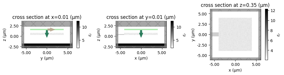
Let's create some initial parameters to test our parameterization with.
def make_symmetric_y(arr: np.ndarray) -> np.ndarray:
    """Make an array symmetric in y."""
    return (arr + np.fliplr(arr)) / 2.0


params0_Si = make_symmetric_y(np.random.random((nx_Si, ny_Si, 1)))
params0_SiN = make_symmetric_y(np.random.random((nx_SiN, ny_SiN, 1)))

sim_etch_random = make_sim_with_etch(params0_Si, params0_SiN)

f, axes = f, (ax1, ax2, ax3) = plt.subplots(1, 3, figsize=(10, 4), tight_layout=True)
sim_etch_random.plot_eps(x=0.0 + shift_plot, monitor_alpha=0.0, ax=ax1)
sim_etch_random.plot_eps(y=0.0 + shift_plot, monitor_alpha=0.0, ax=ax2)
sim_etch_random.plot_eps(z=center_Si_z + shift_plot, monitor_alpha=0.0, ax=ax3)

for ax in axes:
    ax.set_aspect("equal")

plt.show()
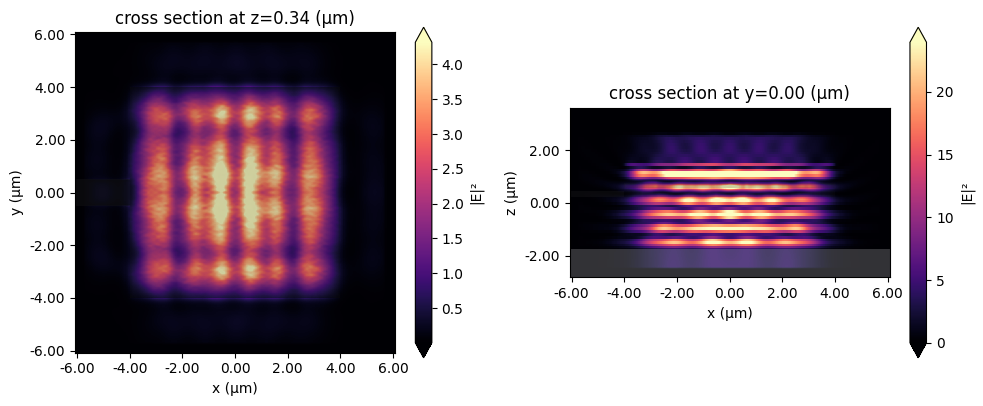
sim_data = web.run(sim_etch_random, task_name="check fields")
17:11:55 -03 Created task 'check fields' with resource_id
             'fdve-9a52c9b1-32bc-464b-81c7-578a9a212ea0' and task_type 'FDTD'.
             View task using web UI at
             'https://tidy3d.simulation.cloud/workbench?taskId=fdve-9a52c9b1-32b
             c-464b-81c7-578a9a212ea0'.
Task folder: 'default'.
Output()
17:12:00 -03 Estimated FlexCredit cost: 1.315. Minimum cost depends on task
             execution details. Use 'web.real_cost(task_id)' to get the billed
             FlexCredit cost after a simulation run.
17:12:02 -03 status = queued
             To cancel the simulation, use 'web.abort(task_id)' or
             'web.delete(task_id)' or abort/delete the task in the web UI.
             Terminating the Python script will not stop the job running on the
             cloud.
Output()
17:12:26 -03 status = preprocess
17:12:34 -03 starting up solver
running solver
Output()
17:12:56 -03 early shutoff detected at 8%, exiting.
17:12:57 -03 status = postprocess
Output()
17:13:00 -03 status = success
17:13:02 -03 View simulation result at
             'https://tidy3d.simulation.cloud/workbench?taskId=fdve-9a52c9b1-32b
             c-464b-81c7-578a9a212ea0'.
Output()
17:13:08 -03 Loading simulation from simulation_data.hdf5
f, (ax1, ax2) = plt.subplots(1, 2, figsize=(10, 4), tight_layout=True)

sim_data.plot_field("field_xy", field_name="E", val="abs^2", ax=ax1)
sim_data.plot_field("field_xz", field_name="E", val="abs^2", ax=ax2)

plt.show()
Define Objective Function
The next step involves defining our objective function, which we seek to maximize with respect to the parameters.
We'll compute the coupling efficiency for the grating coupler, and also include a penalty for each of the design regions depending on how well they satisfy minimum feature size criteria.
from tidy3d.plugins.autograd import make_erosion_dilation_penalty

penalty_fn_Si = make_erosion_dilation_penalty(
    radius_Si, pixel_size_Si, beta=beta_penalty
)
penalty_fn_SiN = make_erosion_dilation_penalty(
    radius_SiN, pixel_size_SiN, beta=beta_penalty
)


def penalty_Si(params: np.ndarray) -> float:
    """Define the erosion dilation invariance penalty for Si density parameters."""
    density = get_density_Si(params)
    return penalty_fn_Si(density)


def penalty_SiN(params: np.ndarray) -> float:
    """Define the erosion dilation invariance penalty for SiN density parameters."""
    density = get_density_SiN(params)
    return penalty_fn_SiN(density)


def coupling_efficiency(sim_data: td.SimulationData) -> float:
    """Coupling efficiency into the waveguide as a function of the simulation output data."""
    output_amps = sim_data["mode"].amps
    amp = output_amps.sel(direction="-", f=freq, mode_index=0).values
    return np.sum(np.abs(amp) ** 2)
def objective(
    params_Si: np.ndarray,
    params_SiN,
    verbose: bool = False,
    include_field_mnts: bool = False,
) -> float:
    """Combined objective function over the full set of parameters."""

    # coupling efficiency calculation, through a differentiable simulation
    sim = make_sim_with_etch(params_Si, params_SiN)
    if not include_field_mnts:
        sim = sim.updated_copy(monitors=[mode_monitor])
    data = web.run(sim, task_name="coupler", verbose=verbose)
    efficiency = coupling_efficiency(data)

    # fabrication penalty calculation for both design regions
    penalty_val_Si = penalty_Si(params_Si)
    penalty_val_SiN = penalty_SiN(params_SiN)

    # total objective (to maximize)
    coupling_objective = 2 * efficiency
    penalty_objective = 0.5 * (penalty_val_Si + penalty_val_SiN)
    return coupling_objective - penalty_objective
Let's test this out and inspect the gradients for each design region as a function of space.
val_grad_fn = autograd.value_and_grad(objective, argnum=(0, 1))
val, grads = val_grad_fn(params0_Si, params0_SiN, verbose=True)
17:13:14 -03 Created task 'coupler' with resource_id
             'fdve-5c72b55f-e0b8-4e2b-a590-e988a131ae34' and task_type 'FDTD'.
             View task using web UI at
             'https://tidy3d.simulation.cloud/workbench?taskId=fdve-5c72b55f-e0b
             8-4e2b-a590-e988a131ae34'.
Task folder: 'default'.
Output()
Output()
17:13:23 -03 Estimated FlexCredit cost: 1.314. Minimum cost depends on task
             execution details. Use 'web.real_cost(task_id)' to get the billed
             FlexCredit cost after a simulation run.
17:13:26 -03 status = queued
             To cancel the simulation, use 'web.abort(task_id)' or
             'web.delete(task_id)' or abort/delete the task in the web UI.
             Terminating the Python script will not stop the job running on the
             cloud.
Output()
17:14:19 -03 status = preprocess
17:14:30 -03 starting up solver
running solver
Output()
17:15:10 -03 early shutoff detected at 8%, exiting.
17:15:11 -03 status = postprocess
Output()
17:15:17 -03 status = success
17:15:19 -03 View simulation result at
             'https://tidy3d.simulation.cloud/workbench?taskId=fdve-5c72b55f-e0b
             8-4e2b-a590-e988a131ae34'.
Output()
17:15:23 -03 Loading simulation from simulation_data.hdf5
17:15:25 -03 Started working on Batch containing 1 tasks.
17:15:34 -03 Maximum FlexCredit cost: 1.338 for the whole batch.
             Use 'Batch.real_cost()' to get the billed FlexCredit cost after
             completion.
Output()
17:17:43 -03 Batch complete.
Output()
grad_Si, grad_SiN = grads

print(f"objective function value = {val}")

f, (ax1, ax2) = plt.subplots(1, 2, figsize=(10, 4), tight_layout=True)

vmag1 = np.max(abs(grad_Si))
im1 = ax1.imshow(np.flipud(np.squeeze(grad_Si)).T, cmap="PiYG", vmax=vmag1, vmin=-vmag1)
plt.colorbar(im1, ax=ax1)
ax1.set_title("gradient w.r.t. Si parameters")

vmag2 = np.max(abs(grad_SiN))
im2 = ax2.imshow(
    np.flipud(np.squeeze(grad_SiN)).T, cmap="PiYG", vmax=vmag2, vmin=-vmag2
)
plt.colorbar(im2, ax=ax2)
ax2.set_title("gradient w.r.t. SiN parameters")

plt.show()
objective function value = -0.8576056156314273
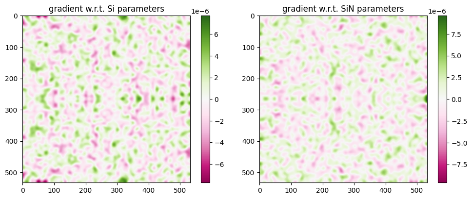
For reference: The green regions represent where we would need to locally increase parameters to increase the objective function and the purple regions represent where we would need to locally decrease parameters to increase our objective function.
Optimization
Let's use our objective function gradient calculator to perform optimization. Like in the adjoint notebooks, we use optax to do Adam optimization in a for loop, feeding it our gradient computed at each iteration.
import optax
# hyperparameters
num_steps = 30
learning_rate = 0.25
def flatten_arrays(arr_Si: np.ndarray, arr_SiN: np.ndarray) -> np.ndarray:
"""Put arr into a 1D array for optax."""
return np.concatenate([arr_Si.flatten(), arr_SiN.flatten()])
def unflatten_array(arr: np.ndarray) -> tuple[np.ndarray, np.ndarray]:
"""Unflatten flattened array into Si and SiN arrays."""
arr_Si = arr[: params0_Si.size].reshape(params0_Si.shape)
arr_SiN = arr[params0_Si.size :].reshape(params0_SiN.shape)
return arr_Si, arr_SiN
def plot_density(density: np.ndarray, ax):
"""Plot the density of the device."""
arr = np.flipud(1 - density.squeeze().T)
ax.imshow(arr, cmap="gray", vmin=0, vmax=1, interpolation="none")
return ax
params = flatten_arrays(params0_Si, params0_SiN)
# initialize adam optimizer with starting parameters (all combined)
optimizer = optax.adam(learning_rate=learning_rate)
opt_state = optimizer.init(params)
# store history
objective_values_history = []
params_history = [(params0_Si, params0_SiN)]
# optimization loop
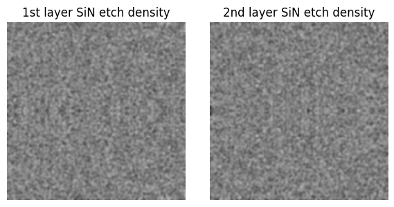
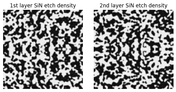
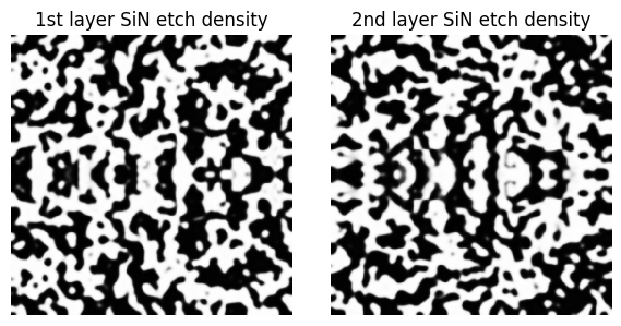
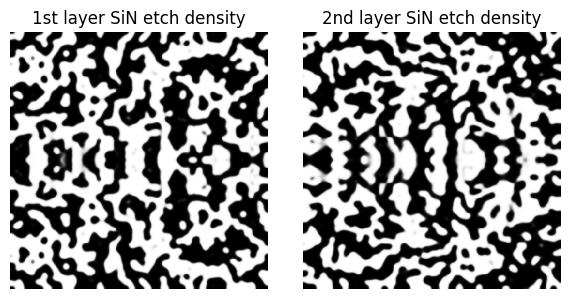
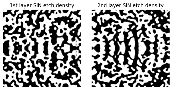
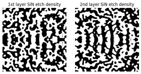
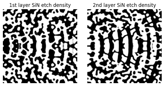
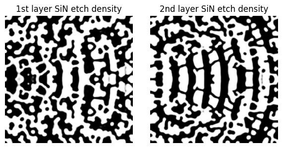
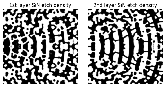
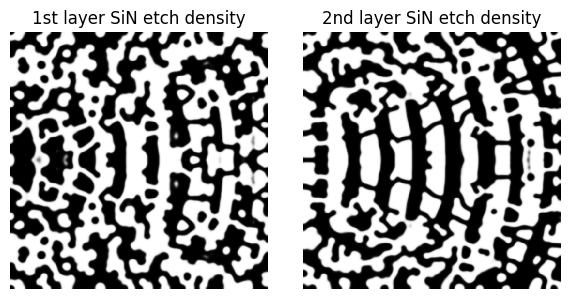
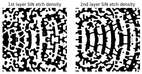
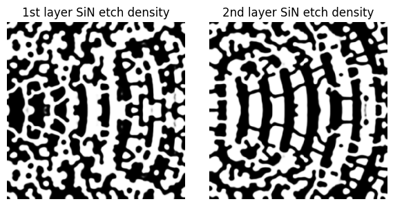
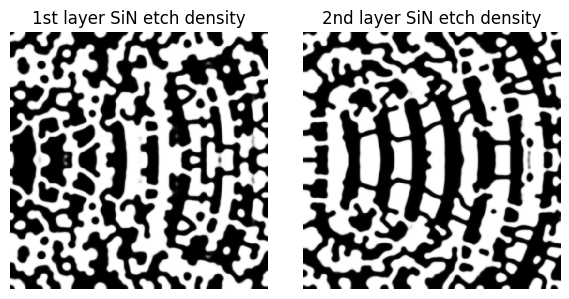
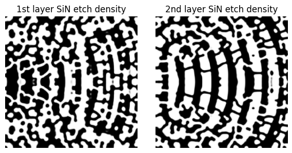
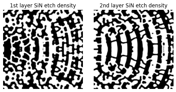
for i in range(num_steps):
# unpack parameters
params_Si, params_SiN = unflatten_array(np.array(params))
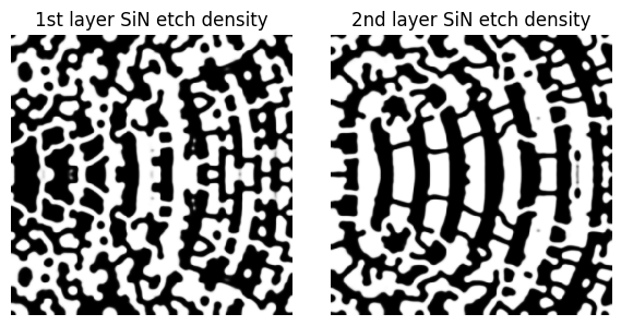
# plot the densities, to monitor
f, (ax1, ax2) = plt.subplots(1, 2, figsize=(6, 3), constrained_layout=True)
plot_density(get_density_Si(params_Si), ax=ax1)
plot_density(get_density_SiN(params_SiN), ax=ax2)
ax1.set_title("1st layer SiN etch density")
ax2.set_title("2nd layer SiN etch density")
ax1.axis("off")
ax2.axis("off")
plt.tight_layout()
plt.show()
val, grads = val_grad_fn(params_Si, params_SiN, verbose=False)
grad_Si, grad_SiN = grads
gradient = flatten_arrays(grad_Si, grad_SiN)
# outputs
print(f"step = {i + 1}")
print(f"\tobjective = {val:.4e}")
print(f"\tgrad_norm = {np.linalg.norm(gradient):.4e}")
# compute and apply updates to the optimizer based on gradient (-1 sign to maximize obj_fn)
updates, opt_state = optimizer.update(-gradient, opt_state, params)
params[:] = optax.apply_updates(params, updates)
# clip the parameters between 0 and 1
np.clip(params, 0.0, 1.0, out=params)
# save history
objective_values_history.append(val)
params_history.append((params_Si, params_SiN))
/tmp/ipykernel_528331/2794811127.py:51: UserWarning: The figure layout has changed to tight
  plt.tight_layout()
step = 1
	objective = -8.5761e-01
	grad_norm = 1.2146e-03
/tmp/ipykernel_528331/2794811127.py:51: UserWarning: The figure layout has changed to tight
  plt.tight_layout()
step = 2
	objective = -2.1726e-01
	grad_norm = 3.4353e-03
/tmp/ipykernel_528331/2794811127.py:51: UserWarning: The figure layout has changed to tight
  plt.tight_layout()
step = 3
	objective = -1.0602e-02
	grad_norm = 2.3649e-03
/tmp/ipykernel_528331/2794811127.py:51: UserWarning: The figure layout has changed to tight
  plt.tight_layout()
step = 4
	objective = 7.2262e-02
	grad_norm = 2.1261e-03
/tmp/ipykernel_528331/2794811127.py:51: UserWarning: The figure layout has changed to tight
  plt.tight_layout()

step = 5
	objective = 1.2171e-01
	grad_norm = 1.5815e-03
/tmp/ipykernel_528331/2794811127.py:51: UserWarning: The figure layout has changed to tight
  plt.tight_layout()
step = 6
	objective = 1.5734e-01
	grad_norm = 1.4110e-03
/tmp/ipykernel_528331/2794811127.py:51: UserWarning: The figure layout has changed to tight
  plt.tight_layout()
step = 7
	objective = 1.8667e-01
	grad_norm = 1.3241e-03
/tmp/ipykernel_528331/2794811127.py:51: UserWarning: The figure layout has changed to tight
  plt.tight_layout()

step = 8
	objective = 2.1199e-01
	grad_norm = 1.3963e-03
/tmp/ipykernel_528331/2794811127.py:51: UserWarning: The figure layout has changed to tight
  plt.tight_layout()

step = 9
	objective = 2.3580e-01
	grad_norm = 1.3241e-03
/tmp/ipykernel_528331/2794811127.py:51: UserWarning: The figure layout has changed to tight
  plt.tight_layout()

step = 10
	objective = 2.5621e-01
	grad_norm = 1.2723e-03
/tmp/ipykernel_528331/2794811127.py:51: UserWarning: The figure layout has changed to tight
  plt.tight_layout()
step = 11
	objective = 2.7261e-01
	grad_norm = 1.4131e-03
/tmp/ipykernel_528331/2794811127.py:51: UserWarning: The figure layout has changed to tight
  plt.tight_layout()

step = 12
	objective = 2.8878e-01
	grad_norm = 1.1688e-03
/tmp/ipykernel_528331/2794811127.py:51: UserWarning: The figure layout has changed to tight
  plt.tight_layout()
step = 13
	objective = 3.0244e-01
	grad_norm = 1.1158e-03
/tmp/ipykernel_528331/2794811127.py:51: UserWarning: The figure layout has changed to tight
  plt.tight_layout()

step = 14
	objective = 3.1503e-01
	grad_norm = 9.9998e-04
/tmp/ipykernel_528331/2794811127.py:51: UserWarning: The figure layout has changed to tight
  plt.tight_layout()
step = 15
	objective = 3.2623e-01
	grad_norm = 9.5212e-04
/tmp/ipykernel_528331/2794811127.py:51: UserWarning: The figure layout has changed to tight
  plt.tight_layout()
step = 16
	objective = 3.3558e-01
	grad_norm = 1.1616e-03
/tmp/ipykernel_528331/2794811127.py:51: UserWarning: The figure layout has changed to tight
  plt.tight_layout()
step = 17
	objective = 3.4581e-01
	grad_norm = 9.1945e-04
/tmp/ipykernel_528331/2794811127.py:51: UserWarning: The figure layout has changed to tight
  plt.tight_layout()

step = 18
	objective = 3.5438e-01
	grad_norm = 9.1020e-04
/tmp/ipykernel_528331/2794811127.py:51: UserWarning: The figure layout has changed to tight
  plt.tight_layout()
step = 19
	objective = 3.6262e-01
	grad_norm = 8.9368e-04
/tmp/ipykernel_528331/2794811127.py:51: UserWarning: The figure layout has changed to tight
  plt.tight_layout()

step = 20
	objective = 3.7062e-01
	grad_norm = 8.7069e-04
/tmp/ipykernel_528331/2794811127.py:51: UserWarning: The figure layout has changed to tight
  plt.tight_layout()
step = 21
	objective = 3.7830e-01
	grad_norm = 8.9552e-04
/tmp/ipykernel_528331/2794811127.py:51: UserWarning: The figure layout has changed to tight
  plt.tight_layout()

step = 22
	objective = 3.8570e-01
	grad_norm = 1.0551e-03
/tmp/ipykernel_528331/2794811127.py:51: UserWarning: The figure layout has changed to tight
  plt.tight_layout()
step = 23
	objective = 3.9316e-01
	grad_norm = 9.5659e-04
/tmp/ipykernel_528331/2794811127.py:51: UserWarning: The figure layout has changed to tight
  plt.tight_layout()
step = 24
	objective = 3.9980e-01
	grad_norm = 8.3652e-04
/tmp/ipykernel_528331/2794811127.py:51: UserWarning: The figure layout has changed to tight
  plt.tight_layout()

step = 25
	objective = 4.0547e-01
	grad_norm = 8.2160e-04
/tmp/ipykernel_528331/2794811127.py:51: UserWarning: The figure layout has changed to tight
  plt.tight_layout()

step = 26
	objective = 4.1068e-01
	grad_norm = 7.7011e-04
/tmp/ipykernel_528331/2794811127.py:51: UserWarning: The figure layout has changed to tight
  plt.tight_layout()
step = 27
	objective = 4.1535e-01
	grad_norm = 7.5375e-04
/tmp/ipykernel_528331/2794811127.py:51: UserWarning: The figure layout has changed to tight
  plt.tight_layout()

step = 28
	objective = 4.1970e-01
	grad_norm = 7.3866e-04
/tmp/ipykernel_528331/2794811127.py:51: UserWarning: The figure layout has changed to tight
  plt.tight_layout()

step = 29
	objective = 4.2380e-01
	grad_norm = 7.1678e-04
/tmp/ipykernel_528331/2794811127.py:51: UserWarning: The figure layout has changed to tight
  plt.tight_layout()

step = 30
	objective = 4.2755e-01
	grad_norm = 7.3870e-04
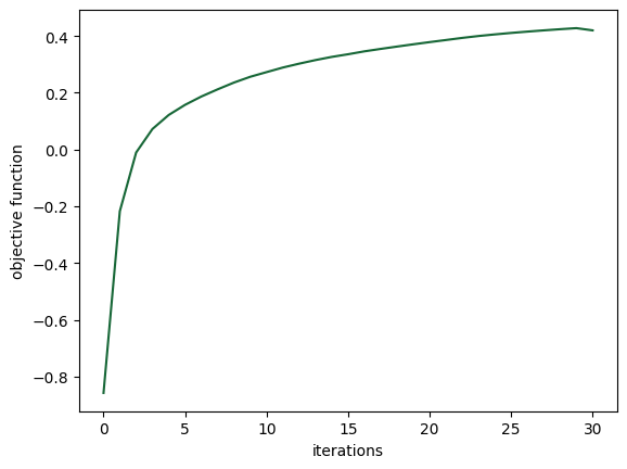
Analysis
Let's compute the objective for the last set of parameters and plot our results.
params_final = params_history[-3]
objective_value_final = objective(*params_final)
objective_values_history.append(objective_value_final)
plt.plot(objective_values_history)
plt.xlabel("iterations")
plt.ylabel("objective function")
plt.show()
sim_final = make_sim_with_etch(*params_final)
sim_data_final = web.run(sim_final, task_name="coupler final")
19:08:07 -03 Created task 'coupler final' with resource_id
             'fdve-19b7fe3d-61dd-46c5-a4fe-756b82bc70a6' and task_type 'FDTD'.
             View task using web UI at
             'https://tidy3d.simulation.cloud/workbench?taskId=fdve-19b7fe3d-61d
             d-46c5-a4fe-756b82bc70a6'.
Task folder: 'default'.
Output()
19:08:12 -03 Estimated FlexCredit cost: 1.315. Minimum cost depends on task
             execution details. Use 'web.real_cost(task_id)' to get the billed
             FlexCredit cost after a simulation run.
19:08:14 -03 status = queued
             To cancel the simulation, use 'web.abort(task_id)' or
             'web.delete(task_id)' or abort/delete the task in the web UI.
             Terminating the Python script will not stop the job running on the
             cloud.
Output()
19:08:46 -03 status = preprocess
19:08:57 -03 starting up solver
running solver
Output()
19:10:34 -03 early shutoff detected at 8%, exiting.
19:10:35 -03 status = postprocess
Output()
19:10:38 -03 status = success
19:10:41 -03 View simulation result at
             'https://tidy3d.simulation.cloud/workbench?taskId=fdve-19b7fe3d-61d
             d-46c5-a4fe-756b82bc70a6'.
Output()
19:10:46 -03 Loading simulation from simulation_data.hdf5
f, ((ax1, ax2), (ax3, ax4)) = plt.subplots(2, 2, figsize=(12, 8), tight_layout=False)

params_Si, params_SiN = params_final
density_Si = get_density_Si(params_Si)
density_SiN = get_density_SiN(params_SiN)

ax1.imshow(np.flipud(1 - density_Si.squeeze().T), cmap="gray")
ax2.imshow(np.flipud(1 - density_SiN.squeeze().T), cmap="gray")
ax1.set_title("Si etch pattern")
ax2.set_title("SiN etch pattern")

sim_data_final.plot_field("field_xy", field_name="E", val="abs^2", ax=ax3)
sim_data_final.plot_field("field_xz", field_name="E", val="abs^2", ax=ax4)
ax3.set_title("intensity coupler (xy) plane")
ax4.set_title("intensity side (xz) plane")

plt.show()
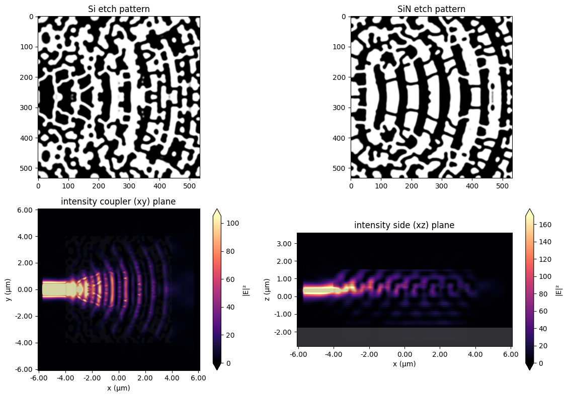
efficiency_final = coupling_efficiency(sim_data_final)
print(f"final coupling efficiency = {100 * efficiency_final:.3f}%")

penalty_val_Si = penalty_Si(params_Si)
penalty_val_SiN = penalty_SiN(params_SiN)
print(f"final penalty (Si) = {penalty_val_Si:.3f}")
print(f"final penalty (SiN) = {penalty_val_SiN:.3f}")
final coupling efficiency = 23.034%
final penalty (Si) = 0.033
final penalty (SiN) = 0.049
# optionally save the coupler history if we want to load it later.
# import pickle
# with open("coupler.pkl", "wb") as file:
#    pickle.dump(params_history, file)