Author: Abhishek Das, North Carolina State University
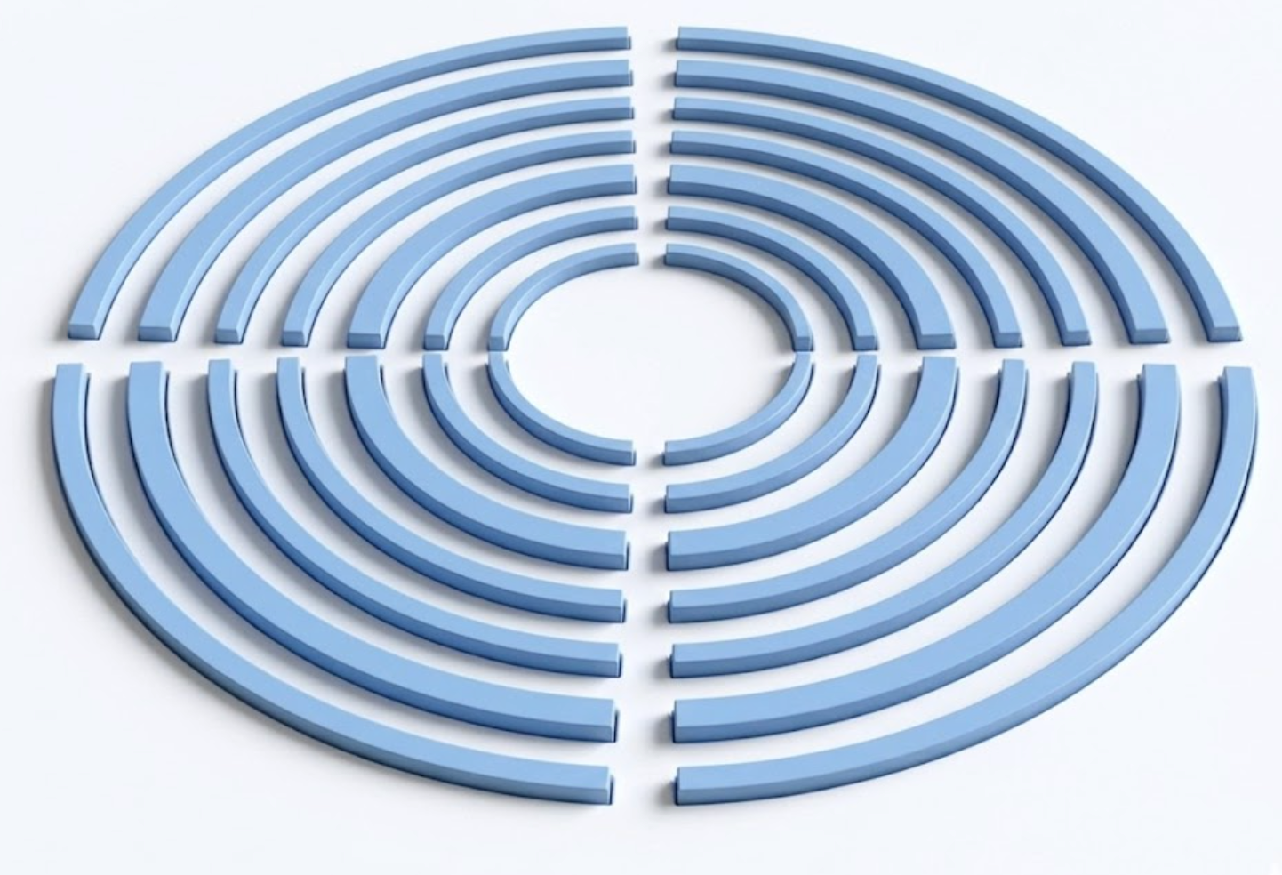
In this notebook, we simulate a bullseye grating on a GaAs slab using Tidy3D. A point dipole source excites the structure, and the far-field radiation pattern is computed to evaluate Gaussian mode overlap and power collection efficiency within a target numerical aperture. Resonance analysis is also performed to identify the high-Q modes of the structure.
The bullseye geometry is defined using GDS (gdstk) and imported into Tidy3D.
[1]:
import numpy as np
import matplotlib.pyplot as plt
import tidy3d as td
import tidy3d.web as web
from tidy3d.plugins.resonance import ResonanceFinder

import gdstk
Set Up the Simulation
[2]:
lambda_min = 0.8
lambda_max = 1.1

monitor_lambda = np.linspace(lambda_min, lambda_max, 401)
monitor_freq = td.constants.C_0 / monitor_lambda
[3]:
automesh_per_wvl = 40
sim_size = Lx, Ly, Lz = (5.5, 5.5, 2)
offset_monitor = 0.4
[4]:
vacuum = td.Medium(permittivity = 1, name = 'vacuum')
GaAs_permittivity = 3.55**2
GaAs = td.Medium(permittivity = GaAs_permittivity, name = 'GaAs')
[5]:
freq0  = 302.675e12
fwidth = 144.131e12

dipole_source = td.PointDipole(
    center = (0, 0, 0),
    source_time = td.GaussianPulse(
        freq0 = freq0,
        fwidth = fwidth
    ),
    polarization = 'Ex',
    name = 'dipole_source'
)
[6]:
t_start = 10/fwidth
t_stop  = 30e-12
Define Structures
[7]:
slab_side_length = 5
slab_height = 0.2
slab = td.Structure(
    geometry = td.Box(
        center = (0, 0, 0),
        size = (slab_side_length, slab_side_length, slab_height),
    ),
    medium = GaAs
)
[8]:
lib = gdstk.Library()
cell = lib.new_cell("BULLSEYE")

central_inner_radius = 0.355 + 0.014
ring_width = 0.07 + np.array([-0.036, -0.015, +0.011, -0.009, -0.011, +0.012, +0.005])
ring_height = 0.2
ring_period = 0.1075

angle = 3
quadrants = 4
theta1 = angle * np.pi / 180
theta2 = (90 - angle) * np.pi / 180

ring_numbers  = np.size(ring_width)

x_origin = 0
y_origin = 0

inner_radius = central_inner_radius

for i in range(ring_numbers):

    outer_radius = inner_radius + ring_width[i]

    for j in range(quadrants):

      gc_slice = gdstk.ellipse(
          (x_origin, y_origin),
          inner_radius,
          outer_radius,
          theta1 + j*np.pi/2,
          theta2 + j*np.pi/2,
          layer = 1,
          datatype = 1,
          tolerance = 0.0001
      )
      cell.add(gc_slice)

    inner_radius = outer_radius + ring_period

gc_etch = td.Geometry.from_gds(
      cell,
      gds_layer = 1,
      axis = 2,
      slab_bounds = (-ring_height/2, ring_height/2)
  )
[9]:
etch = td.Structure(
    geometry = gc_etch,
    medium = vacuum,
    name = "etch"
)
Define Monitor
[10]:
time_monitor_1 = td.FieldTimeMonitor(
    name = "time_monitor_1",
    size = [0.0, 0.0, 0.0],
    center = [0.1, 0.1, 0.0],
    start = t_start
)

time_monitor_2 = td.FieldTimeMonitor(
    name = "time_monitor_2",
    size = [0.0, 0.0, 0.0],
    center = [0.1, 0.2, 0.0],
    start = t_start
)

time_monitor_3 = td.FieldTimeMonitor(
    name = "time_monitor_3",
    size = [0.0, 0.0, 0.0],
    center = [0.2, 0.2, 0.0],
    start = t_start
)

time_monitor_4 = td.FieldTimeMonitor(
    name = "time_monitor_4",
    size = [0.0, 0.0, 0.0],
    center = [0.2, 0.1, 0.0],
    start = t_start
)

time_monitors = [time_monitor_1, time_monitor_2, time_monitor_3, time_monitor_4]
[11]:
far_field_monitor = td.FieldProjectionAngleMonitor(
    center = (0.0, 0.0, offset_monitor),
    size = (td.inf, td.inf, 0),
    name = 'far_field_monitor',
    freqs = monitor_freq,
    normal_dir = '+',
    phi = np.linspace(0, 2*np.pi, 361),
    theta = np.linspace(0, np.pi, 181)
)
Create the Simulation
[12]:
sim = td.Simulation(
    center = (0.0, 0.0, 0.0),
    size = sim_size,
    grid_spec = td.GridSpec.auto(
        wavelength = (lambda_min + lambda_max)/2,
        min_steps_per_wvl = automesh_per_wvl
    ),
    run_time = t_stop,
    sources = [dipole_source],
    monitors = time_monitors + [far_field_monitor],
    structures = [slab, etch],
    medium = vacuum,
    shutoff = 1e-7,
    symmetry = [-1, 1, 0]
)
17:18:20 EDT WARNING: Structure: simulation.structures[0] (no `name` was
             specified) was detected as being less than half of a central
             wavelength from a PML on side x-min. To avoid inaccurate results or
             divergence, please increase gap between any structures and PML or
             fully extend structure through the pml.
WARNING: Suppressed 3 WARNING messages.
             WARNING: Field projection monitor 'far_field_monitor' has
             observation points set up such that the monitor is projecting
             backwards with respect to its 'normal_dir'. If this was not
             intentional, please take a look at the documentation associated
             with this type of projection monitor to check how the observation
             point coordinate system is defined.
[13]:
def gaussian_far_field_no_polarization_sin_debye_apod(theta, phi, NA, n=1.0):

    """
    Compute an ideal far-field Gaussian beam profile with Debye apodization,
    given the theta and phi angles, numerical aperture (NA), and refractive index (n).
    Parameters:
    phi, theta : 1D arrays (rad)
        Input angular coordinates
    NA, n : float
        Numerical aperture and refractive index (of air)
    Returns:
    A : 2D array
        Ideal far-field amplitude profile with Debye apodization
    """
    theta_vals = np.asarray(theta)
    phi_vals   = np.asarray(phi)

    theta_grid, phi_grid = np.meshgrid(theta_vals, phi_vals, indexing='ij')

    # Gaussian term
    gauss = np.exp(-(np.sin(theta_grid) / NA)**2)

    # Debye apodization with safe clipping
    apod = np.sqrt(np.clip(np.cos(theta_grid), 0, None))

    return gauss * apod
[14]:
def compute_gaussian_overlap_without_pol(
    phi, theta, vals,
    NA = 0.68,
    n = 1.0,
    theta_max_deg = None,
    gauss_func = gaussian_far_field_no_polarization_sin_debye_apod,
):
    """
    Compute the mode-overlap between the simulated far-field intensity (vals)
    and an ideal Gaussian far-field WITHOUT polarization effects.

    Overlap is computed as:
        | ∫ E_sim E_gauss dΩ|^2 / ( ∫|E_sim|^2 dΩ  ∫|E_gauss|^2 dΩ )

    Added FEATURE:
        If theta_max_deg is provided (in degrees), the integrals are evaluated
        ONLY for theta <= theta_max_deg.

    Parameters
    ----------
    phi, theta : 1D arrays (rad)
        Angular sampling coordinates of the simulated far-field.
    vals : 2D array
        Simulated intensity map, shape = (len(theta), len(phi)).
    NA, n : floats
        Gaussian beam NA and refractive index.
    theta_max_deg : float or None
        Upper limit of theta (in degrees) for restricting the overlap region.
        If None → use entire theta-domain.
    gauss_func : callable
        Function that generates the ideal Gaussian amplitude:
            gauss_func(theta, phi, NA, n) -> 2D array (len(theta), len(phi))

    Returns
    -------
    percentage_overlap : float
        Mode overlap (0–100%).
    """

    # Convert inputs to arrays
    phi   = np.asarray(phi)
    theta = np.asarray(theta)
    vals  = np.asarray(vals)

    assert vals.shape == (len(theta), len(phi)), \
        f"vals has shape {vals.shape}, but expected {(len(theta), len(phi))}"

    # --- Choose which Gaussian model to use via gauss_func ---
    E_gauss = gauss_func(theta, phi, NA, n)
    I_gauss = E_gauss**2

    # Sim amplitude = sqrt(intensity)
    I_sim = vals
    E_sim = np.sqrt(I_sim)

    # Meshgrid for solid-angle element
    theta_grid, phi_grid = np.meshgrid(theta, phi, indexing='ij')

    # Solid angle element (assume uniform grid)
    dtheta = float(np.mean(np.diff(theta)))
    dphi   = float(np.mean(np.diff(phi)))
    dOmega = np.sin(theta_grid) * dtheta * dphi

    # --------------------------------------
    #  Mask to restrict region if requested
    # --------------------------------------
    if theta_max_deg is not None:
        theta_max_rad = np.radians(theta_max_deg)
        mask = theta_grid <= theta_max_rad
    else:
        mask = np.ones_like(theta_grid, dtype=bool)

    # Apply mask
    E_sim_m   = E_sim[mask]
    E_gauss_m = E_gauss[mask]
    I_sim_m   = I_sim[mask]
    I_gauss_m = I_gauss[mask]
    dOmega_m  = dOmega[mask]

    # --------------------------
    #  Mode overlap numerator
    # --------------------------
    overlap = np.sum(E_sim_m * E_gauss_m * dOmega_m)
    numerator = np.abs(overlap)**2

    # --------------------------
    #  Normalization denominator
    # --------------------------
    norm_sim   = np.sum(I_sim_m   * dOmega_m)
    norm_gauss = np.sum(I_gauss_m * dOmega_m)
    denominator = norm_sim * norm_gauss

    eta = numerator / denominator if denominator > 0 else 0.0
    return float(100 * eta)
[15]:
def compute_power_fraction_and_ratio(
    phi, theta, vals,
    NA_target,
    NA_gauss=0.68,
    n=1.0,
    theta_max_deg=None,
    gauss_func=gaussian_far_field_no_polarization_sin_debye_apod,
):
    r"""
    Compute the percentage of power captured within a target NA cone for:
      (1) simulated far-field intensity vals(θ,φ)
      (2) ideal Gaussian (amplitude) generated by gauss_func

    Then compute the ratio:
        ratio = (percent_sim / percent_gauss)

    Power is integrated over solid angle:
        P \propto \iint I(θ,φ) sinθ dθ dφ

    Optional FEATURE:
        If theta_max_deg is provided, both total-power integrals are computed
        only over θ <= theta_max_deg (same as your overlap style).

    Parameters
    ----------
    phi, theta : 1D arrays (rad)
    vals : 2D array
        Simulated intensity map, shape = (len(theta), len(phi)).
    NA_target : float
        NA defining the capture cone for the fraction calculation.
    NA_gauss : float
        NA used to *define the Gaussian model* in gauss_func (beam divergence).
    n : float
        Refractive index of surrounding medium for θ = asin(NA/n).
    theta_max_deg : float or None
        If provided, restrict all integrals to θ <= theta_max_deg.
    gauss_func : callable
        Gaussian amplitude model:
            gauss_func(theta, phi, NA_gauss, n) -> 2D amplitude array

    Returns
    -------
    percent_sim : float
        0–100 (%) power fraction within NA_target for simulated intensity.
    percent_gauss : float
        0–100 (%) power fraction within NA_target for Gaussian intensity |E|^2.
    ratio : float
        (percent_sim / percent_gauss); np.inf if percent_gauss == 0.
    """

    if gauss_func is None:
        raise ValueError("gauss_func must be provided (it should return Gaussian amplitude).")

    # Convert inputs to arrays
    phi   = np.asarray(phi)
    theta = np.asarray(theta)
    vals  = np.asarray(vals)

    assert vals.shape == (len(theta), len(phi)), \
        f"vals has shape {vals.shape}, but expected {(len(theta), len(phi))}"

    # --- Build Gaussian intensity from amplitude ---
    E_gauss = gauss_func(theta, phi, NA_gauss, n)
    I_gauss = np.abs(E_gauss)**2

    # Simulated intensity
    I_sim = vals

    # Meshgrid for solid-angle element (assume uniform grid like your function)
    theta_grid, phi_grid = np.meshgrid(theta, phi, indexing='ij')

    dtheta = float(np.mean(np.diff(theta)))
    dphi   = float(np.mean(np.diff(phi)))
    dOmega = np.sin(theta_grid) * dtheta * dphi

    # --------------------------------------
    # Masks: (A) optional theta restriction
    # --------------------------------------
    if theta_max_deg is not None:
        theta_max_rad = np.radians(theta_max_deg)
        mask_theta = theta_grid <= theta_max_rad
    else:
        mask_theta = np.ones_like(theta_grid, dtype=bool)

    # --------------------------------------
    # Masks: (B) NA capture cone restriction
    # --------------------------------------
    theta_cap = np.arcsin(np.clip(NA_target / float(n), -1.0, 1.0))
    mask_cap = theta_grid <= theta_cap

    # Combined masks
    mask_total = mask_theta
    mask_in    = mask_theta & mask_cap

    # --------------------------
    # Simulated power fractions
    # --------------------------
    P_sim_total = np.sum(I_sim[mask_total] * dOmega[mask_total])
    P_sim_in    = np.sum(I_sim[mask_in]    * dOmega[mask_in])

    frac_sim = (P_sim_in / P_sim_total) if P_sim_total > 0 else 0.0

    # --------------------------
    # Gaussian power fractions
    # --------------------------
    P_g_total = np.sum(I_gauss[mask_total] * dOmega[mask_total])
    P_g_in    = np.sum(I_gauss[mask_in]    * dOmega[mask_in])

    frac_gauss = (P_g_in / P_g_total) if P_g_total > 0 else 0.0

    percent_sim   = 100.0 * float(frac_sim)
    percent_gauss = 100.0 * float(frac_gauss)
    ratio = np.inf if percent_gauss == 0 else (percent_sim / percent_gauss)

    return percent_sim, percent_gauss, float(ratio)
[16]:
def make_far_field_plot_without_pol(phi, theta, vals, NA = 0.68, n=1.0,
                                    gauss_func = gaussian_far_field_no_polarization_sin_debye_apod,
                                    calculate_overlap=True):
    """
    Plots the far-field intensity distribution, optionally saving the figure and calculating the mode overlap and mentioning it on the plot.
    Parameters:
    theta, phi : 1D arrays (rad)
        Input angular coordinates
    vals : 2D array
        Far-field intensity values
    NA, n : float
        Numerical aperture and refractive index (of air)
    calculate_overlap : bool
        Whether to calculate and display the mode overlap (Ideally when plotting the Gaussian beam, this should be False)
    """

    phi = np.asarray(phi)
    theta = np.asarray(theta)
    vals = np.asarray(vals)
    assert vals.shape == (len(theta), len(phi))

    if calculate_overlap:
        overlap = compute_gaussian_overlap_without_pol(
            phi, theta, vals,
            NA=NA, n=n,
            gauss_func=gauss_func
        )


    I = vals
    I_norm = I / (I.max() if I.max()>0 else 1.0)

    PHI, THETA = np.meshgrid(phi, theta, indexing = 'xy')

    theta_NA_deg = np.degrees(np.arcsin(min(NA/float(n), 1.0)))
    phi_circle = np.linspace(0, 2.0 * np.pi, 721)
    theta_circle = np.full_like(phi_circle, theta_NA_deg)

    fig1, ax1 = plt.subplots(subplot_kw={'projection': 'polar'}, figsize = (6.5,5.5))
    ax1.tick_params(axis='y', colors='white')
    pcm1 = ax1.pcolormesh(PHI, np.degrees(THETA), I_norm, shading='auto', cmap='magma')
    cbar1 = fig1.colorbar(pcm1, ax=ax1, label=r"$|E|^2$")
    ax1.set_ylim(0, 90)
    #ax1.set_title('Far_field: Normalized Intensity')
    ax1.plot(phi_circle, theta_circle, 'w--', lw = 2, label=f'NA={NA:.2f}, n = {n}')
    ax1.legend(loc='upper right')
    if calculate_overlap:
        ax1.text(0.02, 0.98, f'Mode overlap: {overlap:.2f}%', transform = ax1.transAxes, va = 'top', ha = 'left',
                bbox = dict(boxstyle = 'round, pad = 0.3', facecolor = 'black', alpha = 0.55), color = 'white')

    fig1.tight_layout()
    plt.show()
    return
[17]:
task_id = web.upload(sim, task_name = "Inverse_Designed_19th_Obj_6th_Stage_From_Epoch=5_Epoch=15_Rounded_UP_APW=40_T=30")
             WARNING: Simulation has 2.36e+06 time steps. The 'run_time' may be
             unnecessarily large, unless there are very long-lived resonances.
17:18:21 EDT Created task
             'Inverse_Designed_19th_Obj_6th_Stage_From_Epoch=5_Epoch=15_Rounded_
             UP_APW=40_T=30' with resource_id
             'fdve-054f38e1-2068-451e-b2a4-266ac88da4c4' and task_type 'FDTD'.
             View task using web UI at
             'https://tidy3d.simulation.cloud/workbench?taskId=fdve-054f38e1-206
             8-451e-b2a4-266ac88da4c4'.
Task folder: 'default'.
Output()
17:18:23 EDT Estimated FlexCredit cost: 24.324. Minimum cost depends on task
             execution details. Use 'web.real_cost(task_id)' to get the billed
             FlexCredit cost after a simulation run.
Run the Simulation
[18]:
web.start(task_id)
web.monitor(task_id, verbose = True)
17:18:24 EDT status = success
[19]:
sim_data = web.load(task_id, verbose=False, path = "Inverse_Designed_19th_Obj_6th_Stage_From_Epoch=5_Epoch=15_Rounded_UP_APW=40_T=30.hdf5")
print(sim_data.log)
17:18:58 EDT WARNING: Structure: simulation.structures[0] (no `name` was
             specified) was detected as being less than half of a central
             wavelength from a PML on side x-min. To avoid inaccurate results or
             divergence, please increase gap between any structures and PML or
             fully extend structure through the pml.
WARNING: Suppressed 3 WARNING messages.
             WARNING: Field projection monitor 'far_field_monitor' has
             observation points set up such that the monitor is projecting
             backwards with respect to its 'normal_dir'. If this was not
             intentional, please take a look at the documentation associated
             with this type of projection monitor to check how the observation
             point coordinate system is defined.
             WARNING: Simulation final field decay value of 4.6e-07 is greater
             than the simulation shutoff threshold of 1e-07. Consider running
             the simulation again with a larger 'run_time' duration for more
             accurate results.
             WARNING: Warning messages were found in the solver log. For more
             information, check 'SimulationData.log' or use
             'web.download_log(task_id)'.
[18:45:02] WARNING: Structure: simulation.structures[0] (no `name` was
           specified) was detected as being less than half of a central
           wavelength from a PML on side x-min. To avoid inaccurate results or
           divergence, please increase gap between any structures and PML or
           fully extend structure through the pml.
           WARNING: Suppressed 3 WARNING messages.
           WARNING: Field projection monitor 'far_field_monitor' has observation
           points set up such that the monitor is projecting backwards with
           respect to its 'normal_dir'. If this was not intentional, please take
           a look at the documentation associated with this type of projection
           monitor to check how the observation point coordinate system is
           defined.
           USER: Simulation domain Nx, Ny, Nz: [800, 800, 134]
           USER: Applied symmetries: (-1, 1, 0)
           USER: Number of computational grid points: 2.1978e+07.
           USER: Subpixel averaging method: SubpixelSpec(attrs={},
           dielectric=PolarizedAveraging(attrs={}, type='PolarizedAveraging'),
           metal=Staircasing(attrs={}, type='Staircasing'),
           pec=PECConformal(attrs={}, type='PECConformal',
           timestep_reduction=0.3, edge_singularity_correction=True),
           pmc=Staircasing(attrs={}, type='Staircasing'),
           lossy_metal=SurfaceImpedance(attrs={}, type='SurfaceImpedance',
           timestep_reduction=0.0, edge_singularity_correction=True),
           type='SubpixelSpec')
           USER: Number of time steps: 2.3613e+06
           USER: Automatic shutoff factor: 1.00e-07
           USER: Time step (s): 1.2705e-17
           USER:

           USER: Compute source modes time (s):     0.1242
[18:45:03] USER: Rest of setup time (s):            0.9249
[18:45:31] USER: Compute monitor modes time (s):    0.0001
[20:15:58] USER: Solver time (s):                   5450.9610
           USER: Time-stepping speed (cells/s):     1.00e+10
[20:16:07] USER: Post-processing time (s):          8.4307

 ====== SOLVER LOG ======

Processing grid and structures...
Building FDTD update coefficients...
Solver setup time (s):             25.1779

Running solver for 2361336 time steps...
- Time step    435 / time 5.53e-15s (  0 % done), field decay: 1.00e+00
- Time step  94453 / time 1.20e-12s (  4 % done), field decay: 2.82e-03
- Time step 188906 / time 2.40e-12s (  8 % done), field decay: 7.30e-05
- Time step 283360 / time 3.60e-12s ( 12 % done), field decay: 1.63e-03
- Time step 377813 / time 4.80e-12s ( 16 % done), field decay: 4.25e-04
- Time step 472267 / time 6.00e-12s ( 20 % done), field decay: 3.74e-04
- Time step 566720 / time 7.20e-12s ( 24 % done), field decay: 7.02e-04
- Time step 661174 / time 8.40e-12s ( 28 % done), field decay: 8.19e-06
- Time step 755627 / time 9.60e-12s ( 32 % done), field decay: 3.99e-04
- Time step 850080 / time 1.08e-11s ( 36 % done), field decay: 1.34e-04
- Time step 944534 / time 1.20e-11s ( 40 % done), field decay: 7.57e-05
- Time step 1038987 / time 1.32e-11s ( 44 % done), field decay: 1.88e-04
- Time step 1133441 / time 1.44e-11s ( 48 % done), field decay: 3.73e-06
- Time step 1227894 / time 1.56e-11s ( 52 % done), field decay: 9.55e-05
- Time step 1322348 / time 1.68e-11s ( 56 % done), field decay: 4.35e-05
- Time step 1416801 / time 1.80e-11s ( 60 % done), field decay: 1.47e-05
- Time step 1511255 / time 1.92e-11s ( 64 % done), field decay: 4.99e-05
- Time step 1605708 / time 2.04e-11s ( 68 % done), field decay: 1.88e-06
- Time step 1700161 / time 2.16e-11s ( 72 % done), field decay: 2.25e-05
- Time step 1794615 / time 2.28e-11s ( 76 % done), field decay: 1.29e-05
- Time step 1889068 / time 2.40e-11s ( 80 % done), field decay: 2.70e-06
- Time step 1983522 / time 2.52e-11s ( 84 % done), field decay: 1.29e-05
- Time step 2077975 / time 2.64e-11s ( 88 % done), field decay: 8.37e-07
- Time step 2172429 / time 2.76e-11s ( 92 % done), field decay: 5.02e-06
- Time step 2266882 / time 2.88e-11s ( 96 % done), field decay: 3.75e-06
- Time step 2361335 / time 3.00e-11s (100 % done), field decay: 4.60e-07
Time-stepping time (s):            5186.8286
Field projection time (s):         232.2404
Data write time (s):               6.7131
[20]:
sim_data = td.SimulationData.from_file(fname = "Inverse_Designed_19th_Obj_6th_Stage_From_Epoch=5_Epoch=15_Rounded_UP_APW=40_T=30.hdf5")
17:18:59 EDT WARNING: Structure: simulation.structures[0] (no `name` was
             specified) was detected as being less than half of a central
             wavelength from a PML on side x-min. To avoid inaccurate results or
             divergence, please increase gap between any structures and PML or
             fully extend structure through the pml.
WARNING: Suppressed 3 WARNING messages.
             WARNING: Field projection monitor 'far_field_monitor' has
             observation points set up such that the monitor is projecting
             backwards with respect to its 'normal_dir'. If this was not
             intentional, please take a look at the documentation associated
             with this type of projection monitor to check how the observation
             point coordinate system is defined.
Analyze Results
[21]:
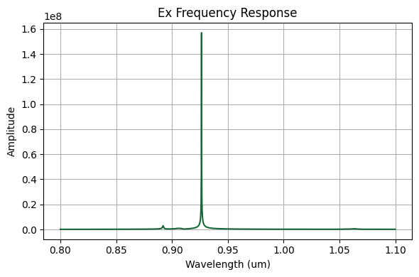
fig, ax = plt.subplots(1, 1, tight_layout = True, figsize = (6,4))

time_monitor_names = [monitor.name for monitor in time_monitors]

time_response_Ex = np.zeros_like(sim_data["time_monitor_1"].Ex.squeeze())

for monitor_name in time_monitor_names:
  time_response_Ex += sim_data[monitor_name].Ex.squeeze()

time_response_Ex /= len(time_monitor_names)

freq_response_Ex = np.abs(np.fft.fft(time_response_Ex))

freqs_Ex = np.linspace(0, 1/sim_data.simulation.dt, len(time_response_Ex))
wavelengths_Ex = td.constants.C_0 / freqs_Ex

plot_inds_Ex = np.where((monitor_freq[-1] < freqs_Ex) & (freqs_Ex < monitor_freq[0]))

ax.plot(wavelengths_Ex[plot_inds_Ex], freq_response_Ex[plot_inds_Ex])
ax.set_xlabel("Wavelength (um)")
ax.set_ylabel("Amplitude")
ax.set_title("Ex Frequency Response")
ax.grid(True)
plt.show()
/var/folders/qn/syhrzy8n7930sgqvxv2x65s40000gn/T/ipykernel_59250/3831151282.py:15: RuntimeWarning: divide by zero encountered in divide
  wavelengths_Ex = td.constants.C_0 / freqs_Ex
[22]:
resonance_finder = ResonanceFinder(freq_window = (monitor_freq[-1], monitor_freq[0]))
resonance_data = resonance_finder.run(signals = sim_data.data)
df_actual = resonance_data.to_dataframe().reset_index()
df_actual['wavelength'] = td.constants.C_0 / df_actual['freq']
print(df_actual[['freq', 'wavelength', 'decay', 'Q', 'amplitude', 'phase', 'error']])
           freq  wavelength         decay            Q   amplitude     phase  \
0  2.699416e+14    1.110583  2.142817e+12   395.762551   30.476848  2.108739
1  2.746487e+14    1.091549  2.879579e+12   299.638982   41.040942 -2.805304
2  2.833892e+14    1.057883  1.830160e+12   486.456684   12.831113 -3.017307
3  3.235854e+14    0.926471  1.137087e+11  8940.158494  254.820183 -0.476974
4  3.298842e+14    0.908781  3.083029e+12   336.150431   88.478080 -0.707611
5  3.309785e+14    0.905776  3.699974e+12   281.028907   99.558649  0.086578
6  3.360605e+14    0.892079  9.866268e+11  1070.075330  160.566584  0.696290
7  3.525750e+14    0.850294  2.285641e+12   484.611064    8.606144  1.830012
8  4.125453e+14    0.726690  1.534290e+12   844.722658  418.070821 -2.465529

      error
0  0.004749
1  0.006332
2  0.006637
3  0.000090
4  0.004032
5  0.005352
6  0.001005
7  0.007987
8  0.002071
[23]:
indices = np.where((monitor_lambda >= 0.92) & (monitor_lambda <=0.93))[0]
for idx in indices:
    print(f"Index: {idx}, Wavelength: {monitor_lambda[idx]:.6f} um")
Index: 160, Wavelength: 0.920000 um
Index: 161, Wavelength: 0.920750 um
Index: 162, Wavelength: 0.921500 um
Index: 163, Wavelength: 0.922250 um
Index: 164, Wavelength: 0.923000 um
Index: 165, Wavelength: 0.923750 um
Index: 166, Wavelength: 0.924500 um
Index: 167, Wavelength: 0.925250 um
Index: 168, Wavelength: 0.926000 um
Index: 169, Wavelength: 0.926750 um
Index: 170, Wavelength: 0.927500 um
Index: 171, Wavelength: 0.928250 um
Index: 172, Wavelength: 0.929000 um
Index: 173, Wavelength: 0.929750 um
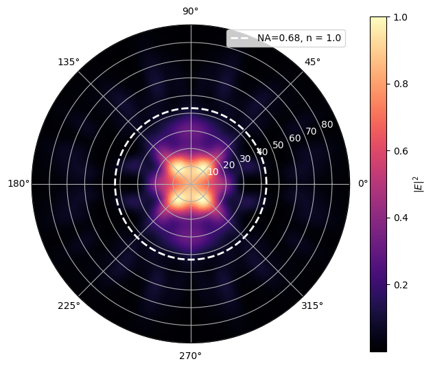
Far-Field Analysis
[24]:
f_index = 168
far_field_data = sim_data[far_field_monitor.name]
Etheta = far_field_data.Etheta.isel(f = f_index, r=0).values
Ephi = far_field_data.Ephi.isel(f = f_index, r=0).values
phi_vals = far_field_data.phi
theta_vals = far_field_data.theta
[25]:
intensity = np.abs(Etheta)**2 + np.abs(Ephi)**2
[26]:
compute_gaussian_overlap_without_pol(
    phi_vals, theta_vals, intensity,
    NA = 0.68, n = 1.0,
    gauss_func=gaussian_far_field_no_polarization_sin_debye_apod
)
[26]:
86.88443254695612
[27]:
p_sim, p_g, r = compute_power_fraction_and_ratio(
    phi_vals, theta_vals, vals=intensity,
    NA_target=0.68,
    NA_gauss=0.68,
    n=1.0,
    theta_max_deg=90,
    gauss_func=gaussian_far_field_no_polarization_sin_debye_apod
)

print(p_sim, p_g, r)
76.16387279212572 87.2671390916859 0.8727669267592844
[28]:
make_far_field_plot_without_pol(
    phi_vals, theta_vals, intensity,
    NA = 0.68, n=1.0,
    gauss_func=gaussian_far_field_no_polarization_sin_debye_apod,
    calculate_overlap=False
)