Author: Amir Targholizadeh Affiliation: QUTECH Lab (Prof. Pankaj K. Jha), Department of Electrical Engineering and Computer Science, Syracuse University Reference: A. Targholizadeh, A. Nikulin, and P. K. Jha, "Cryogenic Dielectric Metasurface-Integrated Superconducting Nanowire Single-Photon Detectors," arXiv:2512.17115 (2025).
Abstract¶
Superconducting nanowire single-photon detectors (SNSPDs) are the leading photon-counting technology for quantum optics, quantum communication, and lidar. However, their performance is constrained by a fundamental tradeoff: small detection areas yield low timing jitter but couple poorly to a free-space beam, while large detection areas couple well but suffer from kinetic-inductance-limited timing jitter.
This notebook reproduces the FDTD design and analysis of a cryogenic silicon metasurface placed in front of a small NbTiN meander to overcome that tradeoff. We cover two complementary devices:
- Focusing metalens — concentrates a 60 × 60 µm² collection aperture down to a 5 × 5 µm² nanowire footprint. We sweep numerical aperture (NA) and report transmission, coupling efficiency, absorption efficiency, and the resulting system-detection-efficiency (SDE) enhancement factor.
-
Polarization beam splitter (PBS) metasurface — uses anisotropic (rectangular) meta-atoms to focus orthogonal linear polarizations onto two spatially separated meanders. We sweep the focal-spot half-separation
dand report intended/unintended absorption and the resulting polarization cross-talk in dB.
Both designs use eight 45° phase bins of pre-optimized dielectric meta-atoms on a thin SiO₂ substrate, with the entire detector enclosed in a quarter-wave cavity bounded above by a PEC mirror. All simulations run with tidy3d.web.run. Note: running the full notebook end-to-end consumes FlexCredits — each NA sweep launches thirteen 3D FDTD jobs (one per NA value, plus a third optional focal-finder sweep), and the PBS sweep launches twelve more (six separations × two polarizations).
1. Setup¶
We start with the standard Python and Tidy3D imports, plus a few configuration globals used throughout the notebook.
import os
import numpy as np
import pandas as pd
import xarray as xr
import matplotlib as mpl
import matplotlib.pyplot as plt
from matplotlib.patches import Circle
from matplotlib.collections import PatchCollection
from mpl_toolkits.axes_grid1 import make_axes_locatable

import tidy3d as td
import tidy3d.web as web

# Output directories
DATA_DIR = "data"
FIG_DIR  = "figs"
os.makedirs(DATA_DIR, exist_ok=True)
os.makedirs(FIG_DIR,  exist_ok=True)

# Publication-style matplotlib defaults
mpl.rcParams.update({
    "font.family":       "DejaVu Sans",
    "font.size":          12,
    "axes.labelsize":     13,
    "axes.titlesize":     14,
    "xtick.labelsize":    11,
    "ytick.labelsize":    11,
    "legend.fontsize":    11,
    "figure.dpi":        120,
    "savefig.dpi":       300,
    "savefig.bbox":      "tight",
    "axes.linewidth":    1.0,
    "xtick.major.width": 1.0,
    "ytick.major.width": 1.0,
})
1.1 Common Physical Parameters¶
The metalens is patterned on a thin SiO₂ membrane and made of amorphous silicon meta-atoms designed for λ = 1.55 µm. Refractive-index values are chosen for cryogenic operation (≈ 4 K), which slightly shifts the optical constants compared with room temperature.
The NbTiN nanowire is modeled as a lossy dielectric with a fitted permittivity and a finite electrical conductivity σ — this lets us extract the absorbed power directly as
$$ P_\mathrm{abs} \;=\; \tfrac{1}{2}\,\sigma \int_V |E|^2 \, dV $$
integrated over the nanowire volume, given a Tidy3D source normalized to 1 W input.
# --- Wavelength and frequency ---
LDA = 1.55                        # design wavelength (µm)
F0  = td.C_0 / LDA                # design frequency (Hz)

# --- Materials (cryogenic, ~4 K) ---
N_SIO2    = 1.457
N_SILICON = 3.4757

SIO2    = td.Medium(name="sio2",    permittivity=N_SIO2**2)
SILICON = td.Medium(name="silicon", permittivity=N_SILICON**2)

# NbTiN: lossy-dielectric model fitted to cryogenic measurements
# (real part of eps, conductivity sigma) -> P_abs = 0.5 * sigma * |E|^2 (per unit volume)
NBTIN_EPS   = 2.8175
NBTIN_SIGMA = 0.8898
NBTIN       = td.Medium(name="NbTiN",
                        permittivity=NBTIN_EPS,
                        conductivity=NBTIN_SIGMA)

# --- Metalens aperture geometry ---
L_METALENS = 60.0                 # square aperture side (µm)
H_ANT      = 0.85                 # cylinder height for the focusing metalens (µm)
SUB_T      = 0.10                 # SiO2 substrate thickness (µm)

# --- Nanowire (NbTiN meander) geometry ---
NW_T       = 0.008                # nanowire thickness     (8 nm)
NW_W       = 0.100                # nanowire width        (100 nm)
NW_L       = 5.0                  # nanowire length        (5 µm)
NW_N       = int(((NW_L / NW_W) - 1) / 2) + 2      # number of strands per meander
CAVITY_H   = 0.266                # quarter-wave cavity height for the metalens design (µm)

# --- Simulation buffers ---
XY_BUFFER  = 2.0 * LDA            # lateral buffer between metalens edge and PML

print(f"Wavelength       λ = {LDA} µm  (f₀ = {F0:.3e} Hz)")
print(f"Metalens         L = {L_METALENS} µm,  cylinder height = {H_ANT} µm")
print(f"Nanowire meander: {NW_N} strands of {NW_L} µm × {NW_W*1000:.0f} nm × {NW_T*1000:.1f} nm")
print(f"NbTiN model:      ε' = {NBTIN_EPS},  σ = {NBTIN_SIGMA}")
Wavelength       λ = 1.55 µm  (f₀ = 1.934e+14 Hz)
Metalens         L = 60.0 µm,  cylinder height = 0.85 µm
Nanowire meander: 26 strands of 5.0 µm × 100 nm × 8.0 nm
NbTiN model:      ε' = 2.8175,  σ = 0.8898
2. Focusing Metalens Design¶
2.1 Phase Profile¶
For a hyperbolic phase profile centered on the lens, the meta-atom at lateral position (x, y) must imprint a phase
$$ \varphi(x,y) \;=\; -\frac{2\pi}{\lambda}\!\left(\sqrt{x^2 + y^2 + f^2} - f\right) \pmod{2\pi} $$
where f is the back focal length. We discretize this continuous phase into 8 bins of 45° and pick one cylindrical meta-atom geometry per bin.
2.2 Pre-Computed Meta-Atom Library¶
The eight cylinder radii below were pre-computed from a unit-cell RCWA / FDTD phase sweep (not reproduced here for brevity). Each radius produces a transmission with approximately unit amplitude and the listed central phase. For the unit-cell library generation, see the supplementary material of the reference paper.
| bin | φ (deg) | radius (µm) |
|---|---|---|
| 0 | 0–45 | 0.180 |
| 1 | 45–90 | 0.193 |
| 2 | 90–135 | 0.214 |
| 3 | 135–180 | 0.242 |
| 4 | 180–225 | 0.102 |
| 5 | 225–270 | 0.140 |
| 6 | 270–315 | 0.157 |
| 7 | 315–360 | 0.168 |
2.3 The NA Sweep — Note on F_OFFSET_LIST¶
The paraxial back focal length from a hyperbolic phase profile is
$$ f_{00} \;=\; \frac{L/2}{\tan(\arcsin\,\mathrm{NA})} $$
This is only an approximation: at high NA the actual focal plane shifts toward the lens because of finite meta-atom thickness, near-field coupling between adjacent cylinders, and other non-paraxial effects. F_OFFSET_LIST stores the empirical correction $\Delta f$ (in µm) between the paraxial design and the converged focal plane. The simulation then uses
$$ f \;=\; f_{00} - h_\mathrm{ant} - \Delta f $$
as the back-focal distance and places the focal-plane monitor accordingly. The values below are the pre-computed result of the focal-finder sweep in Section 4; running that section overwrites F_OFFSET_LIST with values recomputed from your own FDTD runs. If you trust the pre-computed list, skip Section 4 and proceed straight to Section 5.
# 8-bin meta-atom radii (µm) — pre-computed from unit-cell phase sweep
RADII = np.array([0.180, 0.193, 0.214, 0.242, 0.102, 0.140, 0.157, 0.168])

# NA sweep parameters
NA_LIST       = np.array([0.20, 0.25, 0.30, 0.35, 0.40, 0.45, 0.50,
                          0.55, 0.60, 0.65, 0.70, 0.75, 0.80])

# Empirical focal-plane correction Δf (µm), indexed by NA_LIST.
# The actual focal distance is  f = f00 - h_ant - F_OFFSET_LIST[i].
F_OFFSET_LIST = np.array([24.833, 17.600, 13.725, 10.625,  8.558,  7.008,  5.458,
                           4.425,  3.650,  2.875,  2.093,  1.583,  1.067])

# Meta-atom unit cell (lateral pitch)
CELL_SIZE = 0.6                                   # µm
NUM_CELLS = int(L_METALENS / CELL_SIZE)


def metalens_cylinders(L, na, cell_size, num_cells, radii, lda,
                       sub_z, sub_t, h_ant):
    """
    Build the list of cylindrical meta-atoms for a focusing metalens of side `L`
    at numerical aperture `na`.

    Returns
    -------
    cyls : list[td.Cylinder]
        One cylinder per occupied unit cell, placed on the SiO2 substrate top.
    f00  : float
        Paraxial back focal length (used only for phase-profile evaluation).
    """
    f00 = (L / 2) / np.tan(np.arcsin(na))
    xc  = np.linspace(-L/2 + cell_size/2, L/2 - cell_size/2, num_cells)
    yc  = np.linspace(-L/2 + cell_size/2, L/2 - cell_size/2, num_cells)

    cyls = []
    for x in xc:
        for y in yc:
            phi_deg = np.mod((-2*np.pi/lda *
                              (np.sqrt(x**2 + y**2 + f00**2) - f00)) * 180/np.pi,
                             360)
            bin_idx = int(phi_deg // 45)
            if 0 <= bin_idx < 8:
                cyls.append(td.Cylinder(
                    center=[x, y, sub_z + sub_t/2 + h_ant/2],
                    radius=float(radii[bin_idx]),
                    length=h_ant,
                ))
    return cyls, f00
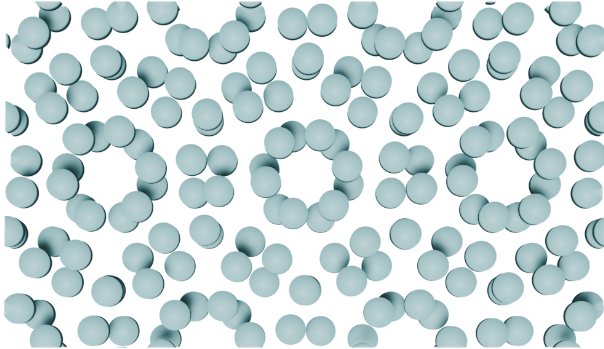
3. Visualizing the Metalens Layout¶
Before launching the FDTD sweep we visualize the meta-atom layout for one representative NA (here NA = 0.5). The figure overlays the continuous hyperbolic phase profile φ(x, y) (rainbow background) with the actual placed cylinders (black circles). This makes it easy to verify by eye that the meta-atoms tile the phase rings as expected.
# Pick one NA for visualization
NA_VIZ   = 0.5
F00_VIZ  = (L_METALENS/2) / np.tan(np.arcsin(NA_VIZ))

# Build the cylinder list (use a dummy sub_z=0 because we only need (x, y, r))
viz_cyls, _ = metalens_cylinders(
    L_METALENS, NA_VIZ, CELL_SIZE, NUM_CELLS, RADII, LDA,
    sub_z=0.0, sub_t=SUB_T, h_ant=H_ANT,
)
ant_x = np.array([c.center[0] for c in viz_cyls])
ant_y = np.array([c.center[1] for c in viz_cyls])
ant_r = np.array([c.radius     for c in viz_cyls])
print(f"NA = {NA_VIZ}: total cylinders placed = {len(viz_cyls)}")

# Continuous phase background on a fine grid
N_BG = 600
x_bg = np.linspace(-L_METALENS/2, L_METALENS/2, N_BG)
y_bg = np.linspace(-L_METALENS/2, L_METALENS/2, N_BG)
Xb, Yb = np.meshgrid(x_bg, y_bg, indexing="xy")
phase_deg = np.mod(-2*np.pi/LDA *
                   (np.sqrt(Xb**2 + Yb**2 + F00_VIZ**2) - F00_VIZ),
                   2*np.pi) * 180/np.pi

# Plot
fig, ax = plt.subplots(figsize=(7.5, 7))
im = ax.imshow(phase_deg,
               extent=[-L_METALENS/2, L_METALENS/2,
                       -L_METALENS/2, L_METALENS/2],
               origin="lower", cmap="rainbow",
               vmin=0, vmax=360, alpha=0.65,
               interpolation="bilinear", zorder=1)

patches = [Circle((xi, yi), ri) for xi, yi, ri in zip(ant_x, ant_y, ant_r)]
pc = PatchCollection(patches, facecolor="black", edgecolor="none",
                     alpha=0.9, zorder=2)
ax.add_collection(pc)

# Aperture outline
ax.plot([-L_METALENS/2, L_METALENS/2, L_METALENS/2, -L_METALENS/2, -L_METALENS/2],
        [-L_METALENS/2, -L_METALENS/2, L_METALENS/2,  L_METALENS/2, -L_METALENS/2],
        "k-", lw=1.0, zorder=3)

cbar = fig.colorbar(im, ax=ax, pad=0.02, fraction=0.046,
                    ticks=[0, 90, 180, 270, 360])
cbar.set_label("Phase φ (°)")

ax.set_xlabel("x (µm)"); ax.set_ylabel("y (µm)")
ax.set_aspect("equal")
ax.set_xlim(-L_METALENS/2, L_METALENS/2)
ax.set_ylim(-L_METALENS/2, L_METALENS/2)
ax.set_title(f"Metalens layout at NA = {NA_VIZ}\n"
             f"{L_METALENS:.0f} × {L_METALENS:.0f} µm² aperture · "
             f"{len(viz_cyls)} meta-atoms")

plt.tight_layout()
plt.savefig(os.path.join(FIG_DIR, f"metalens_layout_NA{NA_VIZ:.2f}.png"))
plt.show()
NA = 0.5: total cylinders placed = 10000
4. Focal-Plane Finder (Optional)¶
The F_OFFSET_LIST defined in Section 2.3 has to come from somewhere. This section is the reproducible recipe that generates it: for each NA in the sweep we run a bare-metalens FDTD simulation (no nanowires) with a line monitor along the optical axis, locate the |E|² peak, and read off the actual focal distance from the antenna top.
The workflow has two parts:
-
4.1 — launch one bare-metalens simulation per NA with an axial
FieldMonitorrunning from just above the antenna top to the top of the simulation box. - 4.2 — load each result, find the peak of $|E_x|^2 + |E_y|^2 + |E_z|^2$ along that line, and compute $\Delta f = f_\mathrm{design,\,top} - f_\mathrm{simulated}$.
This produces a fresh F_OFFSET_LIST from your own simulations rather than relying on the pre-computed numbers in §2.3.
Skip this section to save 13 FlexCredits-worth of simulation time and use the pre-computed list. The downstream sweeps in Sections 5 and 6 read F_OFFSET_LIST regardless of how it was populated.
FlexCredit note: thirteen 3D FDTD simulations (one per NA in NA_LIST).
# --- 4.1: Launch the focal-finder sweep ---
def build_focal_finder_sim(na, L=L_METALENS):
    """
    Bare metalens with an axial line monitor above the antenna top.
    No nanowires, no PEC mirror — pure optical focusing test.
    """
    f00          = (L/2) / np.tan(np.arcsin(na))
    f_design_top = f00 - H_ANT                      # designed distance above antenna

    L_sim_xy = L + 2 * XY_BUFFER

    z_below_sub = 2 * LDA
    z_above     = f_design_top + 1.0
    L_h         = z_below_sub + SUB_T + H_ANT + z_above
    sub_z       = -L_h/2 + z_below_sub + SUB_T/2
    metalens_top = sub_z + SUB_T/2 + H_ANT

    # --- Substrate ---
    metalens_sub = td.Structure(
        geometry=td.Box(center=[0, 0, sub_z],
                        size=[td.inf, td.inf, SUB_T]),
        name="metalens_sub", medium=SIO2,
    )

    # --- Metalens cylinders (with PML-safety filter on positions) ---
    xc = np.linspace(-L/2 + CELL_SIZE/2, L/2 - CELL_SIZE/2, NUM_CELLS)
    yc = np.linspace(-L/2 + CELL_SIZE/2, L/2 - CELL_SIZE/2, NUM_CELLS)
    safe_edge = L_sim_xy/2 - LDA
    max_r     = RADII.max()
    cyls = []
    for x in xc:
        for y in yc:
            if (abs(x) + max_r > safe_edge) or (abs(y) + max_r > safe_edge):
                continue
            phi_deg = np.mod((-2*np.pi/LDA *
                              (np.sqrt(x**2 + y**2 + f00**2) - f00)) * 180/np.pi,
                             360)
            bin_idx = int(phi_deg // 45)
            if 0 <= bin_idx < 8:
                cyls.append(td.Cylinder(
                    center=[x, y, sub_z + SUB_T/2 + H_ANT/2],
                    radius=float(RADII[bin_idx]), length=H_ANT,
                ))
    metalens = td.Structure(
        geometry=td.GeometryGroup(geometries=cyls),
        medium=SILICON, name="metalens",
    )

    # --- Source ---
    src = td.PlaneWave(
        name="x_pol",
        center=[0, 0, sub_z - SUB_T],
        size=[L, L, 0],
        source_time=td.GaussianPulse(freq0=F0, fwidth=F0/5),
        num_freqs=1, direction="+",
    )

    # --- Axial line monitor: x = y = 0, z spanning from above the antenna to top ---
    z_line_min   = metalens_top + 0.1            # 100 nm above antenna
    z_line_max   = metalens_top + z_above
    z_line_cen   = 0.5 * (z_line_min + z_line_max)
    z_line_size  = z_line_max - z_line_min

    axial_line = td.FieldMonitor(
        name="axial_line",
        center=[0, 0, z_line_cen],
        size=[0, 0, z_line_size],
        freqs=[F0],
        fields=["Ex", "Ey", "Ez"],
    )
    field_xz = td.FieldMonitor(
        name="field_xz",
        size=[td.inf, 0, td.inf],
        freqs=[F0],
        fields=["Ex", "Ey", "Ez"],
    )

    sim = td.Simulation(
        size=(L_sim_xy, L_sim_xy, L_h),
        grid_spec=td.GridSpec.auto(wavelength=LDA, min_steps_per_wvl=6),
        structures=[metalens_sub, metalens],
        boundary_spec=td.BoundarySpec(
            x=td.Boundary.pml(),
            y=td.Boundary.pml(),
            z=td.Boundary.pml(),
        ),
        sources=[src],
        monitors=[axial_line, field_xz],
        run_time=2 * L_h * 1e-14,
    )
    return sim, dict(n_cyl=len(cyls), f_design_top=f_design_top,
                     z_line_min=z_line_min, z_line_max=z_line_max,
                     metalens_top=metalens_top)


# Launch all 13 NA values
for na in NA_LIST:
    sim, info = build_focal_finder_sim(na)
    print(f"\n### NA = {na:.2f} ###")
    print(f"  f_design_top = {info['f_design_top']:.3f} µm,  "
          f"line z ∈ [{info['z_line_min']:.2f}, {info['z_line_max']:.2f}] µm")
    print(f"  cylinders = {info['n_cyl']}")

    web.run(
        sim,
        task_name=f"focal_finder_NA{na:.2f}",
        path=os.path.join(DATA_DIR, f"focal_finder_NA{na:.2f}.hdf5"),
        verbose=True,
    )

print("\nAll focal-finder runs complete.")
### NA = 0.20 ###
  f_design_top = 146.119 µm,  line z ∈ [-71.43, 75.58] µm
  cylinders = 10000
13:51:43 -03 Loading simulation from local cache. View cached task using web UI
             at
             'https://tidy3d.simulation.cloud/workbench?taskId=fdve-70294f06-e74
             d-45e1-93b7-1d58eaa03b34'.
### NA = 0.25 ###
  f_design_top = 115.340 µm,  line z ∈ [-56.04, 60.19] µm
  cylinders = 10000
13:51:45 -03 Loading simulation from local cache. View cached task using web UI
             at
             'https://tidy3d.simulation.cloud/workbench?taskId=fdve-44badfd7-0bc
             4-4b79-9f5d-5303a4b102ed'.
13:51:46 -03 WARNING: Simulation final field decay value of 1.17e-05 is greater
             than the simulation shutoff threshold of 1e-05. Consider running
             the simulation again with a larger 'run_time' duration for more
             accurate results.
### NA = 0.30 ###
  f_design_top = 94.544 µm,  line z ∈ [-45.65, 49.80] µm
  cylinders = 10000
13:51:47 -03 Loading simulation from local cache. View cached task using web UI
             at
             'https://tidy3d.simulation.cloud/workbench?taskId=fdve-4f1e7fa3-9a6
             2-4428-be29-7f715897e4f1'.
13:51:48 -03 WARNING: Simulation final field decay value of 2.46e-05 is greater
             than the simulation shutoff threshold of 1e-05. Consider running
             the simulation again with a larger 'run_time' duration for more
             accurate results.
### NA = 0.35 ###
  f_design_top = 79.443 µm,  line z ∈ [-38.10, 42.25] µm
  cylinders = 10000
13:51:49 -03 Loading simulation from local cache. View cached task using web UI
             at
             'https://tidy3d.simulation.cloud/workbench?taskId=fdve-462aa958-fad
             7-46e2-b2d2-b4b349068184'.
13:51:50 -03 WARNING: Simulation final field decay value of 4e-05 is greater
             than the simulation shutoff threshold of 1e-05. Consider running
             the simulation again with a larger 'run_time' duration for more
             accurate results.
### NA = 0.40 ###
  f_design_top = 67.889 µm,  line z ∈ [-32.32, 36.47] µm
  cylinders = 10000
13:51:51 -03 Loading simulation from local cache. View cached task using web UI
             at
             'https://tidy3d.simulation.cloud/workbench?taskId=fdve-d3a65b49-d1b
             d-42c9-a9f6-6b79e9ae8d84'.
13:51:52 -03 WARNING: Simulation final field decay value of 6.55e-05 is greater
             than the simulation shutoff threshold of 1e-05. Consider running
             the simulation again with a larger 'run_time' duration for more
             accurate results.
### NA = 0.45 ###
  f_design_top = 58.685 µm,  line z ∈ [-27.72, 31.87] µm
  cylinders = 10000
13:51:53 -03 Loading simulation from local cache. View cached task using web UI
             at
             'https://tidy3d.simulation.cloud/workbench?taskId=fdve-68d1bda8-14c
             4-4f25-a0e0-4bf11f742a71'.
13:51:54 -03 WARNING: Simulation final field decay value of 0.000124 is greater
             than the simulation shutoff threshold of 1e-05. Consider running
             the simulation again with a larger 'run_time' duration for more
             accurate results.
### NA = 0.50 ###
  f_design_top = 51.112 µm,  line z ∈ [-23.93, 28.08] µm
  cylinders = 10000
13:51:55 -03 Loading simulation from local cache. View cached task using web UI
             at
             'https://tidy3d.simulation.cloud/workbench?taskId=fdve-34490420-69b
             9-47b6-bc6d-ac7a1b6e735d'.
             WARNING: Simulation final field decay value of 0.000191 is greater
             than the simulation shutoff threshold of 1e-05. Consider running
             the simulation again with a larger 'run_time' duration for more
             accurate results.
### NA = 0.55 ###
  f_design_top = 44.704 µm,  line z ∈ [-20.73, 24.88] µm
  cylinders = 10000
13:51:57 -03 Loading simulation from local cache. View cached task using web UI
             at
             'https://tidy3d.simulation.cloud/workbench?taskId=fdve-1d5d2b60-856
             0-4e21-9fc4-8c759cde546f'.
             WARNING: Simulation final field decay value of 0.000325 is greater
             than the simulation shutoff threshold of 1e-05. Consider running
             the simulation again with a larger 'run_time' duration for more
             accurate results.
### NA = 0.60 ###
  f_design_top = 39.150 µm,  line z ∈ [-17.95, 22.10] µm
  cylinders = 10000
13:51:59 -03 Loading simulation from local cache. View cached task using web UI
             at
             'https://tidy3d.simulation.cloud/workbench?taskId=fdve-cb933487-e79
             4-4bf8-a35e-647b7195cf12'.
             WARNING: Simulation final field decay value of 0.000501 is greater
             than the simulation shutoff threshold of 1e-05. Consider running
             the simulation again with a larger 'run_time' duration for more
             accurate results.
### NA = 0.65 ###
  f_design_top = 34.224 µm,  line z ∈ [-15.49, 19.64] µm
  cylinders = 10000
13:52:00 -03 Loading simulation from local cache. View cached task using web UI
             at
             'https://tidy3d.simulation.cloud/workbench?taskId=fdve-a968b5a8-74b
             e-4c45-a275-e705be4465bc'.
13:52:01 -03 WARNING: Simulation final field decay value of 0.000844 is greater
             than the simulation shutoff threshold of 1e-05. Consider running
             the simulation again with a larger 'run_time' duration for more
             accurate results.
### NA = 0.70 ###
  f_design_top = 29.756 µm,  line z ∈ [-13.25, 17.40] µm
  cylinders = 10000
13:52:02 -03 Loading simulation from local cache. View cached task using web UI
             at
             'https://tidy3d.simulation.cloud/workbench?taskId=fdve-e51be414-92f
             9-409a-b67a-3d8bb9c57d18'.
13:52:03 -03 WARNING: Simulation final field decay value of 0.0015 is greater
             than the simulation shutoff threshold of 1e-05. Consider running
             the simulation again with a larger 'run_time' duration for more
             accurate results.
### NA = 0.75 ###
  f_design_top = 25.608 µm,  line z ∈ [-11.18, 15.33] µm
  cylinders = 10000
13:52:04 -03 Loading simulation from local cache. View cached task using web UI
             at
             'https://tidy3d.simulation.cloud/workbench?taskId=fdve-c983a68d-d32
             a-4fa4-a681-f4b72d8ef397'.
13:52:05 -03 WARNING: Simulation final field decay value of 0.00291 is greater
             than the simulation shutoff threshold of 1e-05. Consider running
             the simulation again with a larger 'run_time' duration for more
             accurate results.
### NA = 0.80 ###
  f_design_top = 21.650 µm,  line z ∈ [-9.20, 13.35] µm
  cylinders = 10000
13:52:06 -03 Loading simulation from local cache. View cached task using web UI
             at
             'https://tidy3d.simulation.cloud/workbench?taskId=fdve-e75df85c-918
             9-4a0f-8d4b-90cf9be94945'.
13:52:07 -03 WARNING: Simulation final field decay value of 0.00411 is greater
             than the simulation shutoff threshold of 1e-05. Consider running
             the simulation again with a larger 'run_time' duration for more
             accurate results.
All focal-finder runs complete.
4.1 Post-Process — Locate Peaks and Recompute F_OFFSET_LIST¶
Load each saved focal-finder simulation, find the |E|² peak along the axial line, and convert that to a Δf value relative to the designed (paraxial) focal distance.
LINE_MON = "axial_line"


def _antenna_top_z(sim_data):
    """Recover the antenna-top z-coordinate from the saved simulation geometry."""
    for s in sim_data.simulation.structures:
        if getattr(s, "name", None) == "metalens":
            cyl = s.geometry.geometries[0]
            return cyl.center[2] + cyl.length / 2
    raise RuntimeError("metalens structure not found")


rows = []
for na in NA_LIST:
    path = os.path.join(DATA_DIR, f"focal_finder_NA{na:.2f}.hdf5")
    if not os.path.exists(path):
        print(f"[skip] {path}")
        continue

    sd = td.SimulationData.from_file(path)
    if LINE_MON not in sd.monitor_data:
        print(f"  [warn] '{LINE_MON}' missing in {path}")
        continue

    Ex = sd[LINE_MON].Ex.abs.isel(f=0).squeeze(drop=True)
    Ey = sd[LINE_MON].Ey.abs.isel(f=0).squeeze(drop=True)
    Ez = sd[LINE_MON].Ez.abs.isel(f=0).squeeze(drop=True)
    E2 = (Ex**2 + Ey**2 + Ez**2).values
    z  = sd[LINE_MON].Ex.coords["z"].values

    z_top  = _antenna_top_z(sd)
    z_peak = float(z[int(np.argmax(E2))])
    f_sim  = z_peak - z_top                       # antenna-top -> focus distance

    f00          = (L_METALENS/2) / np.tan(np.arcsin(na))
    f_design_top = f00 - H_ANT
    delta_f      = f_design_top - f_sim
    dff_abs      = abs(delta_f / f_design_top)

    rows.append({
        "NA":           na,
        "z_top":        z_top,
        "z_peak":       z_peak,
        "f_simulated":  f_sim,
        "f_design_top": f_design_top,
        "delta_f":      delta_f,
        "abs_dff":      dff_abs,
    })
    print(f"NA = {na:.2f}:  f_design = {f_design_top:6.3f} µm,  "
          f"f_sim = {f_sim:6.3f} µm,  "
          f"Δf = {delta_f:+6.3f} µm,  |Δf/f| = {dff_abs:.4f}")

df_focal = pd.DataFrame(rows)
df_focal.to_csv(os.path.join(DATA_DIR, "focal_finder_summary.csv"), index=False)

# --- Overwrite F_OFFSET_LIST with the freshly-computed values ---
if len(df_focal) == len(NA_LIST):
    F_OFFSET_LIST = df_focal["delta_f"].to_numpy()
    print(f"\nF_OFFSET_LIST overwritten from focal-finder results.")
else:
    print(f"\n[warn] only {len(df_focal)}/{len(NA_LIST)} runs found — "
          f"keeping pre-computed F_OFFSET_LIST.")

# --- Plot |Δf / f| vs NA ---
fig, ax = plt.subplots(figsize=(7, 5))
ax.plot(df_focal["NA"], df_focal["abs_dff"], "o-", color="#1f4eda", linewidth=2)
ax.set_xlabel("NA")
ax.set_ylabel(r"$|\Delta f / f|$")
ax.set_title("Relative focal-plane shift vs NA")
ax.grid(alpha=0.3)
plt.tight_layout()
plt.savefig(os.path.join(FIG_DIR, "abs_dff_vs_NA.png"))
plt.show()
NA = 0.20:  f_design = 146.119 µm,  f_sim = 121.286 µm,  Δf = +24.833 µm,  |Δf/f| = 0.1700
NA = 0.25:  f_design = 115.340 µm,  f_sim = 97.740 µm,  Δf = +17.600 µm,  |Δf/f| = 0.1526
NA = 0.30:  f_design = 94.544 µm,  f_sim = 80.819 µm,  Δf = +13.725 µm,  |Δf/f| = 0.1452
NA = 0.35:  f_design = 79.443 µm,  f_sim = 68.818 µm,  Δf = +10.625 µm,  |Δf/f| = 0.1337
NA = 0.40:  f_design = 67.889 µm,  f_sim = 59.330 µm,  Δf = +8.558 µm,  |Δf/f| = 0.1261
NA = 0.45:  f_design = 58.685 µm,  f_sim = 51.677 µm,  Δf = +7.008 µm,  |Δf/f| = 0.1194
NA = 0.50:  f_design = 51.112 µm,  f_sim = 45.653 µm,  Δf = +5.458 µm,  |Δf/f| = 0.1068
NA = 0.55:  f_design = 44.704 µm,  f_sim = 40.279 µm,  Δf = +4.425 µm,  |Δf/f| = 0.0990
NA = 0.60:  f_design = 39.150 µm,  f_sim = 35.500 µm,  Δf = +3.650 µm,  |Δf/f| = 0.0932
NA = 0.65:  f_design = 34.224 µm,  f_sim = 31.349 µm,  Δf = +2.875 µm,  |Δf/f| = 0.0840
NA = 0.70:  f_design = 29.756 µm,  f_sim = 27.663 µm,  Δf = +2.093 µm,  |Δf/f| = 0.0703
NA = 0.75:  f_design = 25.608 µm,  f_sim = 24.024 µm,  Δf = +1.583 µm,  |Δf/f| = 0.0618
NA = 0.80:  f_design = 21.650 µm,  f_sim = 20.583 µm,  Δf = +1.067 µm,  |Δf/f| = 0.0493

F_OFFSET_LIST overwritten from focal-finder results.
5. NA Sweep #1 — Transmission and Focal-Spot Coupling (No Nanowires)¶
This first sweep characterizes the optical performance of the bare metalens (no NbTiN, no PEC mirror). For each NA we extract two quantities:
- Transmission $T = P_\mathrm{trans}/P_\mathrm{in}$, integrated over the entire simulation cross-section 400 nm above the metalens. This tells us how much of the input power makes it past the structure at all.
- Coupling efficiency $\eta_c = P_\mathrm{det}/P_\mathrm{in}$, integrated over a 5 × 5 µm² square at the focal plane. This is the fraction of the input that lands on a future SNSPD-sized detector footprint.
The 1 W plane-wave source is sized to the 60 × 60 µm² metalens aperture, so there is no aperture-fraction correction at post-processing.
FlexCredit note: thirteen 3D FDTD simulations are launched here (one per NA value).
def build_metalens_sim_no_wire(na, f_offset, L=L_METALENS, det_w=5.0):
    """
    Build an FDTD simulation for the bare metalens (no nanowires, no PEC).

    Uses f = f00 - h_ant - f_offset as the back focal length.
    """
    # Effective back focal length
    f00 = (L/2) / np.tan(np.arcsin(na))
    f   = f00 - H_ANT - f_offset

    # Lateral simulation size
    L_sim_xy = L + 2 * XY_BUFFER

    # z layout
    z_below_sub = 2 * LDA                                    # source + PML buffer below
    z_above     = f + 1.0                                    # focal plane + 1 µm margin
    L_h         = z_below_sub + SUB_T + H_ANT + z_above
    sub_z       = -L_h/2 + z_below_sub + SUB_T/2
    metalens_top = sub_z + SUB_T/2 + H_ANT
    trans_z     = metalens_top + 0.4                         # 400 nm above metalens
    focal_z     = metalens_top + f                           # focal plane

    # --- Substrate ---
    metalens_sub = td.Structure(
        geometry=td.Box(center=[0, 0, sub_z],
                        size=[td.inf, td.inf, SUB_T]),
        name="metalens_sub", medium=SIO2,
    )

    # --- Metalens cylinders ---
    cyls, _ = metalens_cylinders(L, na, CELL_SIZE, NUM_CELLS, RADII, LDA,
                                 sub_z=sub_z, sub_t=SUB_T, h_ant=H_ANT)
    metalens = td.Structure(
        geometry=td.GeometryGroup(geometries=cyls),
        medium=SILICON, name="metalens",
    )

    # --- Source: plane wave restricted to the metalens aperture ---
    src = td.PlaneWave(
        name="x_pol",
        center=[0, 0, sub_z - SUB_T],
        size=[L, L, 0],
        source_time=td.GaussianPulse(freq0=F0, fwidth=F0/5),
        num_freqs=1, direction="+",
    )

    # --- Monitors ---
    freqs = [F0]
    trans_flux = td.FluxMonitor(
        name="trans_flux",
        center=[0, 0, trans_z],
        size=[L_sim_xy, L_sim_xy, 0],
        freqs=freqs,
    )
    detector_flux = td.FluxMonitor(
        name="detector_flux",
        center=[0, 0, focal_z],
        size=[det_w, det_w, 0],
        freqs=freqs,
    )
    field_xz = td.FieldMonitor(
        name="field_xz",
        size=[td.inf, 0, td.inf],
        freqs=freqs,
        fields=["Ex", "Ey", "Ez"],
    )

    sim = td.Simulation(
        size=(L_sim_xy, L_sim_xy, L_h),
        grid_spec=td.GridSpec.auto(wavelength=LDA, min_steps_per_wvl=6),
        structures=[metalens_sub, metalens],
        boundary_spec=td.BoundarySpec(
            x=td.Boundary.pml(),
            y=td.Boundary.pml(),
            z=td.Boundary.pml(),
        ),
        sources=[src],
        monitors=[trans_flux, detector_flux, field_xz],
        run_time=2 * L_h * 1e-14,
    )
    return sim, dict(L_sim_xy=L_sim_xy, L_h=L_h, sub_z=sub_z,
                     trans_z=trans_z, focal_z=focal_z, n_cyl=len(cyls))


# --- Launch the sweep ---
for na, f_offset in zip(NA_LIST, F_OFFSET_LIST):
    sim, info = build_metalens_sim_no_wire(na, f_offset)
    print(f"\n=== NA = {na:.3f}  f_offset = {f_offset:.2f} µm ===")
    print(f"  L_sim_xy = {info['L_sim_xy']:.2f} µm,  L_h = {info['L_h']:.2f} µm")
    print(f"  trans_z  = {info['trans_z']:.3f} µm,  focal_z = {info['focal_z']:.3f} µm")
    print(f"  cylinders: {info['n_cyl']}")

    web.run(
        sim,
        task_name=f"Tdet_NA{na:.2f}",
        path=os.path.join(DATA_DIR, f"Tdet_NA{na:.2f}.hdf5"),
        verbose=True,
    )

print("\nAll NA-sweep (no-wire) runs complete.")
=== NA = 0.200  f_offset = 24.83 µm ===
  L_sim_xy = 66.20 µm,  L_h = 126.34 µm
  trans_z  = -58.718 µm,  focal_z = 62.168 µm
  cylinders: 10000
13:52:19 -03 Loading simulation from local cache. View cached task using web UI
             at
             'https://tidy3d.simulation.cloud/workbench?taskId=fdve-a3ea025b-20d
             4-4c16-b2a4-33936e4a0e2c'.
13:52:20 -03 WARNING: Simulation final field decay value of 1.56e-05 is greater
             than the simulation shutoff threshold of 1e-05. Consider running
             the simulation again with a larger 'run_time' duration for more
             accurate results.
=== NA = 0.250  f_offset = 17.60 µm ===
  L_sim_xy = 66.20 µm,  L_h = 102.79 µm
  trans_z  = -46.945 µm,  focal_z = 50.395 µm
  cylinders: 10000
13:52:22 -03 Loading simulation from local cache. View cached task using web UI
             at
             'https://tidy3d.simulation.cloud/workbench?taskId=fdve-378ddf03-17e
             5-41fa-952a-a77821be6f92'.
             WARNING: Simulation final field decay value of 2.52e-05 is greater
             than the simulation shutoff threshold of 1e-05. Consider running
             the simulation again with a larger 'run_time' duration for more
             accurate results.
=== NA = 0.300  f_offset = 13.72 µm ===
  L_sim_xy = 66.20 µm,  L_h = 85.87 µm
  trans_z  = -38.484 µm,  focal_z = 41.934 µm
  cylinders: 10000
13:52:23 -03 Loading simulation from local cache. View cached task using web UI
             at
             'https://tidy3d.simulation.cloud/workbench?taskId=fdve-878b9d4a-f7b
             c-4741-9567-1cb786b97ec6'.
13:52:24 -03 WARNING: Simulation final field decay value of 5.11e-05 is greater
             than the simulation shutoff threshold of 1e-05. Consider running
             the simulation again with a larger 'run_time' duration for more
             accurate results.
=== NA = 0.350  f_offset = 10.62 µm ===
  L_sim_xy = 66.20 µm,  L_h = 73.87 µm
  trans_z  = -32.484 µm,  focal_z = 35.934 µm
  cylinders: 10000
13:52:25 -03 Loading simulation from local cache. View cached task using web UI
             at
             'https://tidy3d.simulation.cloud/workbench?taskId=fdve-2c0ad843-bab
             0-42f3-a1fc-e05829a535b0'.
13:52:26 -03 WARNING: Simulation final field decay value of 7.93e-05 is greater
             than the simulation shutoff threshold of 1e-05. Consider running
             the simulation again with a larger 'run_time' duration for more
             accurate results.
=== NA = 0.400  f_offset = 8.56 µm ===
  L_sim_xy = 66.20 µm,  L_h = 64.38 µm
  trans_z  = -27.740 µm,  focal_z = 31.190 µm
  cylinders: 10000
13:52:27 -03 Loading simulation from local cache. View cached task using web UI
             at
             'https://tidy3d.simulation.cloud/workbench?taskId=fdve-10f30b3d-eaf
             6-478f-a1bf-e2b4c18210a1'.
13:52:28 -03 WARNING: Simulation final field decay value of 0.000125 is greater
             than the simulation shutoff threshold of 1e-05. Consider running
             the simulation again with a larger 'run_time' duration for more
             accurate results.
=== NA = 0.450  f_offset = 7.01 µm ===
  L_sim_xy = 66.20 µm,  L_h = 56.73 µm
  trans_z  = -23.913 µm,  focal_z = 27.363 µm
  cylinders: 10000
13:52:29 -03 Loading simulation from local cache. View cached task using web UI
             at
             'https://tidy3d.simulation.cloud/workbench?taskId=fdve-86615d1a-256
             4-4d9b-ab60-7cd067abe051'.
13:52:30 -03 WARNING: Simulation final field decay value of 0.000226 is greater
             than the simulation shutoff threshold of 1e-05. Consider running
             the simulation again with a larger 'run_time' duration for more
             accurate results.
=== NA = 0.500  f_offset = 5.46 µm ===
  L_sim_xy = 66.20 µm,  L_h = 50.70 µm
  trans_z  = -20.902 µm,  focal_z = 24.352 µm
  cylinders: 10000
13:52:31 -03 Loading simulation from local cache. View cached task using web UI
             at
             'https://tidy3d.simulation.cloud/workbench?taskId=fdve-9a6ec854-c86
             9-4fd0-a582-1272bec8a75e'.
13:52:32 -03 WARNING: Simulation final field decay value of 0.000289 is greater
             than the simulation shutoff threshold of 1e-05. Consider running
             the simulation again with a larger 'run_time' duration for more
             accurate results.
=== NA = 0.550  f_offset = 4.43 µm ===
  L_sim_xy = 66.20 µm,  L_h = 45.33 µm
  trans_z  = -18.215 µm,  focal_z = 21.665 µm
  cylinders: 10000
13:52:33 -03 Loading simulation from local cache. View cached task using web UI
             at
             'https://tidy3d.simulation.cloud/workbench?taskId=fdve-3eb4c5b3-417
             c-41f7-a0c6-670e72d138a8'.
13:52:34 -03 WARNING: Simulation final field decay value of 0.000531 is greater
             than the simulation shutoff threshold of 1e-05. Consider running
             the simulation again with a larger 'run_time' duration for more
             accurate results.
=== NA = 0.600  f_offset = 3.65 µm ===
  L_sim_xy = 66.20 µm,  L_h = 40.55 µm
  trans_z  = -15.825 µm,  focal_z = 19.275 µm
  cylinders: 10000
13:52:35 -03 Loading simulation from local cache. View cached task using web UI
             at
             'https://tidy3d.simulation.cloud/workbench?taskId=fdve-64013935-7af
             0-40cc-9e54-99b27bf37801'.
13:52:36 -03 WARNING: Simulation final field decay value of 0.000865 is greater
             than the simulation shutoff threshold of 1e-05. Consider running
             the simulation again with a larger 'run_time' duration for more
             accurate results.
=== NA = 0.650  f_offset = 2.88 µm ===
  L_sim_xy = 66.20 µm,  L_h = 36.40 µm
  trans_z  = -13.749 µm,  focal_z = 17.199 µm
  cylinders: 10000
13:52:37 -03 Loading simulation from local cache. View cached task using web UI
             at
             'https://tidy3d.simulation.cloud/workbench?taskId=fdve-281398e5-90a
             5-45ef-800d-52c142fd98ca'.
13:52:38 -03 WARNING: Simulation final field decay value of 0.00111 is greater
             than the simulation shutoff threshold of 1e-05. Consider running
             the simulation again with a larger 'run_time' duration for more
             accurate results.
=== NA = 0.700  f_offset = 2.09 µm ===
  L_sim_xy = 66.20 µm,  L_h = 32.71 µm
  trans_z  = -11.907 µm,  focal_z = 15.357 µm
  cylinders: 10000
13:52:39 -03 Loading simulation from local cache. View cached task using web UI
             at
             'https://tidy3d.simulation.cloud/workbench?taskId=fdve-6f8786f2-a29
             4-4b9c-966b-84b5d088a5fc'.
13:52:41 -03 WARNING: Simulation final field decay value of 0.00208 is greater
             than the simulation shutoff threshold of 1e-05. Consider running
             the simulation again with a larger 'run_time' duration for more
             accurate results.
=== NA = 0.750  f_offset = 1.58 µm ===
  L_sim_xy = 66.20 µm,  L_h = 29.07 µm
  trans_z  = -10.087 µm,  focal_z = 13.537 µm
  cylinders: 10000
13:52:42 -03 Loading simulation from local cache. View cached task using web UI
             at
             'https://tidy3d.simulation.cloud/workbench?taskId=fdve-46b909ec-ccb
             f-4480-8195-15b03b44db9f'.
13:52:43 -03 WARNING: Simulation final field decay value of 0.00286 is greater
             than the simulation shutoff threshold of 1e-05. Consider running
             the simulation again with a larger 'run_time' duration for more
             accurate results.
=== NA = 0.800  f_offset = 1.07 µm ===
  L_sim_xy = 66.20 µm,  L_h = 25.63 µm
  trans_z  = -8.367 µm,  focal_z = 11.817 µm
  cylinders: 10000
13:52:44 -03 Loading simulation from local cache. View cached task using web UI
             at
             'https://tidy3d.simulation.cloud/workbench?taskId=fdve-9f6f80f8-dfc
             c-4b91-9666-ae6665576a24'.
13:52:45 -03 WARNING: Simulation final field decay value of 0.0059 is greater
             than the simulation shutoff threshold of 1e-05. Consider running
             the simulation again with a larger 'run_time' duration for more
             accurate results.
All NA-sweep (no-wire) runs complete.
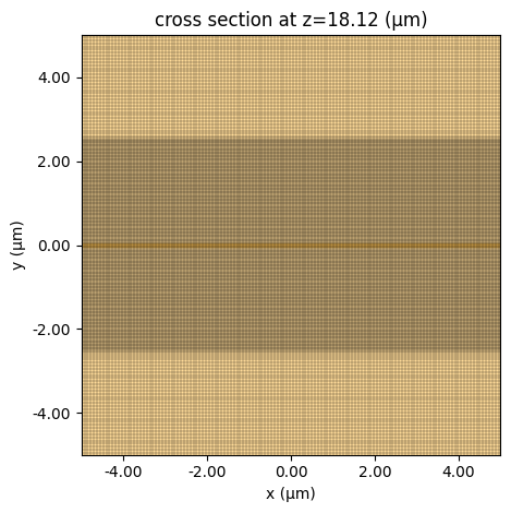
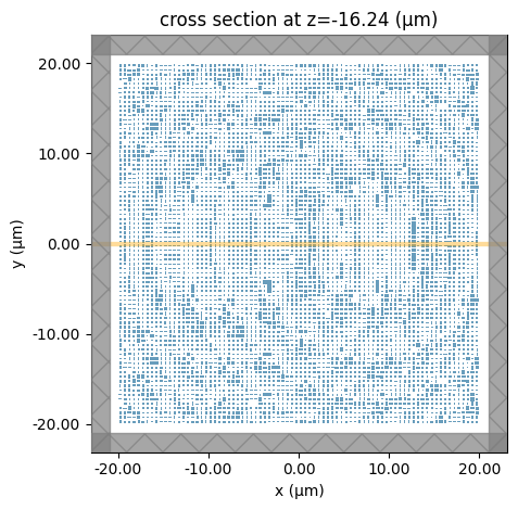
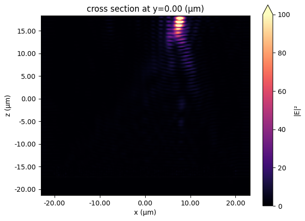
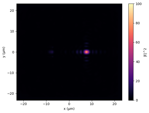
6. NA Sweep #2 — Absorption With NbTiN Nanowire Meander¶
This second sweep places a 5 × 5 µm² NbTiN nanowire meander at the focal plane, inside a thin SiO₂ cavity bounded above by a PEC mirror. The cavity reuses light not absorbed on the first pass, improving overall absorption — this is the standard quarter-wave-cavity geometry for SNSPDs.
We extract the absorbed power by integrating $\tfrac{1}{2}\sigma|E|^2$ over the nanowire volume in post-processing (Section 6).
FlexCredit note: thirteen more 3D FDTD simulations are launched here. The mesh is refined locally to resolve the 8 nm-thick nanowire (MeshOverrideStructure with sub-nm dl along z).
def build_metalens_sim_with_wire(na, f_offset, L=L_METALENS, d_wire=0.0):
    """
    Build an FDTD simulation for the metalens + NbTiN meander in a PEC-capped cavity.

    Uses f = f00 - h_ant - f_offset as the back focal length, identical to the
    no-wire builder so that monitor placement is consistent.

    Parameters
    ----------
    d_wire : float
        Lateral offset of the meander center along x (µm). For the centered
        focusing-only sweep we use d_wire = 0.
    """
    f00 = (L/2) / np.tan(np.arcsin(na))
    f   = f00 - H_ANT - f_offset

    L_sim_xy = L + 2 * XY_BUFFER

    # z layout: cavity top sits exactly at the PEC boundary (no top buffer)
    z_below_sub = 2 * LDA / 3
    L_h         = z_below_sub + SUB_T + H_ANT + f + CAVITY_H
    sub_z       = -L_h/2 + z_below_sub + SUB_T/2
    metalens_top = sub_z + SUB_T/2 + H_ANT
    cavity_z    = metalens_top + f + CAVITY_H/2
    cavity_bot  = cavity_z - CAVITY_H/2
    nanowire_z  = cavity_bot - NW_T/2                       # wire on cavity floor

    # --- Substrate ---
    metalens_sub = td.Structure(
        geometry=td.Box(center=[0, 0, sub_z],
                        size=[td.inf, td.inf, SUB_T]),
        name="metalens_sub", medium=SIO2,
    )

    # --- Metalens cylinders (with PML-safety filter on cylinder positions) ---
    xc  = np.linspace(-L/2 + CELL_SIZE/2, L/2 - CELL_SIZE/2, NUM_CELLS)
    yc  = np.linspace(-L/2 + CELL_SIZE/2, L/2 - CELL_SIZE/2, NUM_CELLS)
    max_r     = RADII.max()
    safe_edge = L_sim_xy/2 - LDA
    cyls = []
    for x in xc:
        for y in yc:
            if (abs(x) + max_r > safe_edge) or (abs(y) + max_r > safe_edge):
                continue
            phi_deg = np.mod((-2*np.pi/LDA *
                              (np.sqrt(x**2 + y**2 + f00**2) - f00)) * 180/np.pi,
                             360)
            bin_idx = int(phi_deg // 45)
            if 0 <= bin_idx < 8:
                cyls.append(td.Cylinder(
                    center=[x, y, sub_z + SUB_T/2 + H_ANT/2],
                    radius=float(RADII[bin_idx]),
                    length=H_ANT,
                ))
    metalens = td.Structure(
        geometry=td.GeometryGroup(geometries=cyls),
        medium=SILICON, name="metalens",
    )

    # --- SiO2 cavity (extends past PEC boundary to avoid edge warning) ---
    cavity_box_h = CAVITY_H + 1.0
    cavity_box_z = cavity_bot + cavity_box_h/2
    cavity = td.Structure(
        geometry=td.Box(center=[0, 0, cavity_box_z],
                        size=[td.inf, td.inf, cavity_box_h]),
        name="cavity", medium=SIO2,
    )

    # --- Nanowire meander (long axis along x) ---
    nw_y0 = -(2*NW_N - 1)*NW_W/2 + NW_W/2
    wires = [
        td.Box(center=[d_wire, nw_y0 + 2*NW_W*n, nanowire_z],
               size=[NW_L, NW_W, NW_T])
        for n in range(NW_N)
    ]
    x_meander = td.Structure(
        geometry=td.GeometryGroup(geometries=wires),
        medium=NBTIN, name="x_meander",
    )

    # --- Source (normalized to 1 W) ---
    src = td.PlaneWave(
        name="x_pol",
        center=[0, 0, sub_z - SUB_T],
        size=[L, L, 0],
        source_time=td.GaussianPulse(freq0=F0, fwidth=F0/5),
        num_freqs=1, direction="+",
    )

    # --- Field monitor over the full meander volume (for absorption integration) ---
    nw_y_total = (2*NW_N - 1)*NW_W + 2*0.02
    nanowire_volume = td.FieldMonitor(
        name="nanowire_volume",
        center=[d_wire, 0, nanowire_z],
        size=[NW_L, nw_y_total, NW_T + 0.02],
        freqs=[F0],
        fields=["Ex", "Ey", "Ez"],
    )
    field_xz = td.FieldMonitor(
        name="field_xz",
        size=[td.inf, 0, td.inf],
        freqs=[F0],
        fields=["Ex", "Ey", "Ez"],
    )

    # --- Local mesh refinement on the wires ---
    nw_refine = td.MeshOverrideStructure(
        geometry=td.Box(center=[d_wire, 0, nanowire_z],
                        size=[NW_L, nw_y_total, NW_T + 0.02]),
        dl=[None, 0.01, 0.002],
    )

    # PEC on the top boundary, PML elsewhere
    boundary_z = td.Boundary(minus=td.PML(), plus=td.PECBoundary())

    sim = td.Simulation(
        size=(L_sim_xy, L_sim_xy, L_h),
        grid_spec=td.GridSpec.auto(
            wavelength=LDA, min_steps_per_wvl=6,
            override_structures=[nw_refine],
        ),
        structures=[metalens_sub, metalens, cavity, x_meander],
        boundary_spec=td.BoundarySpec(
            x=td.Boundary.pml(),
            y=td.Boundary.pml(),
            z=boundary_z,
        ),
        sources=[src],
        monitors=[nanowire_volume, field_xz],
        run_time=2 * L_h * 1e-14,
    )
    return sim, dict(n_cyl=len(cyls), nanowire_z=nanowire_z, L_h=L_h)


# --- Launch the sweep ---
for na, f_offset in zip(NA_LIST, F_OFFSET_LIST):
    sim, info = build_metalens_sim_with_wire(na, f_offset)
    print(f"\n=== NA = {na:.3f}  f_offset = {f_offset:.2f} µm ===")
    print(f"  cylinders = {info['n_cyl']},  L_h = {info['L_h']:.2f} µm")

    web.run(
        sim,
        task_name=f"absorption_NA{na:.2f}",
        path=os.path.join(DATA_DIR, f"absorption_NA{na:.2f}.hdf5"),
        verbose=True,
    )

print("\nAll NA-sweep (with-wire) runs complete.")
=== NA = 0.200  f_offset = 24.83 µm ===
  cylinders = 10000,  L_h = 123.54 µm
13:52:48 -03 Created task 'absorption_NA0.20' with resource_id
             'fdve-592af19f-24fa-432d-9e7f-2a5d759fa32c' and task_type 'FDTD'.
             View task using web UI at
             'https://tidy3d.simulation.cloud/workbench?taskId=fdve-592af19f-24f
             a-432d-9e7f-2a5d759fa32c'.
Task folder: 'default'.
Output()
13:52:55 -03 Estimated FlexCredit cost: 47.206. Minimum cost depends on task
             execution details. Use 'web.real_cost(task_id)' to get the billed
             FlexCredit cost after a simulation run.
13:52:57 -03 status = queued
             To cancel the simulation, use 'web.abort(task_id)' or
             'web.delete(task_id)' or abort/delete the task in the web UI.
             Terminating the Python script will not stop the job running on the
             cloud.
Output()
13:59:31 -03 status = preprocess
13:59:42 -03 starting up solver
running solver
Output()
14:33:58 -03 status = postprocess
Output()
14:34:04 -03 status = success
14:34:06 -03 View simulation result at
             'https://tidy3d.simulation.cloud/workbench?taskId=fdve-592af19f-24f
             a-432d-9e7f-2a5d759fa32c'.
Output()
14:34:28 -03 Loading results from data/absorption_NA0.20.hdf5
14:34:29 -03 WARNING: Simulation final field decay value of 0.00134 is greater
             than the simulation shutoff threshold of 1e-05. Consider running
             the simulation again with a larger 'run_time' duration for more
             accurate results.
=== NA = 0.250  f_offset = 17.60 µm ===
  cylinders = 10000,  L_h = 99.99 µm
14:34:31 -03 Created task 'absorption_NA0.25' with resource_id
             'fdve-8914b5de-76a8-4dee-b211-ec1774c75a72' and task_type 'FDTD'.
             View task using web UI at
             'https://tidy3d.simulation.cloud/workbench?taskId=fdve-8914b5de-76a
             8-4dee-b211-ec1774c75a72'.
Task folder: 'default'.
Output()
14:34:38 -03 Estimated FlexCredit cost: 36.612. Minimum cost depends on task
             execution details. Use 'web.real_cost(task_id)' to get the billed
             FlexCredit cost after a simulation run.
14:34:40 -03 status = queued
             To cancel the simulation, use 'web.abort(task_id)' or
             'web.delete(task_id)' or abort/delete the task in the web UI.
             Terminating the Python script will not stop the job running on the
             cloud.
Output()
14:42:40 -03 status = preprocess
14:42:46 -03 starting up solver
running solver
Output()
14:59:12 -03 status = postprocess
Output()
14:59:15 -03 status = success
14:59:17 -03 View simulation result at
             'https://tidy3d.simulation.cloud/workbench?taskId=fdve-8914b5de-76a
             8-4dee-b211-ec1774c75a72'.
Output()
14:59:35 -03 Loading results from data/absorption_NA0.25.hdf5
14:59:36 -03 WARNING: Simulation final field decay value of 0.00143 is greater
             than the simulation shutoff threshold of 1e-05. Consider running
             the simulation again with a larger 'run_time' duration for more
             accurate results.
=== NA = 0.300  f_offset = 13.72 µm ===
  cylinders = 10000,  L_h = 83.07 µm
14:59:39 -03 Created task 'absorption_NA0.30' with resource_id
             'fdve-1ef93289-bf58-4cc6-ad0f-d2768e8008d9' and task_type 'FDTD'.
             View task using web UI at
             'https://tidy3d.simulation.cloud/workbench?taskId=fdve-1ef93289-bf5
             8-4cc6-ad0f-d2768e8008d9'.
Task folder: 'default'.
Output()
14:59:46 -03 Estimated FlexCredit cost: 29.382. Minimum cost depends on task
             execution details. Use 'web.real_cost(task_id)' to get the billed
             FlexCredit cost after a simulation run.
14:59:48 -03 status = queued
             To cancel the simulation, use 'web.abort(task_id)' or
             'web.delete(task_id)' or abort/delete the task in the web UI.
             Terminating the Python script will not stop the job running on the
             cloud.
Output()
15:00:04 -03 status = preprocess
15:00:17 -03 starting up solver
15:00:18 -03 running solver
Output()
15:17:24 -03 status = postprocess
Output()
15:17:30 -03 status = success
15:17:32 -03 View simulation result at
             'https://tidy3d.simulation.cloud/workbench?taskId=fdve-1ef93289-bf5
             8-4cc6-ad0f-d2768e8008d9'.
Output()
15:17:55 -03 Loading results from data/absorption_NA0.30.hdf5
15:17:56 -03 WARNING: Simulation final field decay value of 0.00185 is greater
             than the simulation shutoff threshold of 1e-05. Consider running
             the simulation again with a larger 'run_time' duration for more
             accurate results.
=== NA = 0.350  f_offset = 10.62 µm ===
  cylinders = 10000,  L_h = 71.07 µm
15:17:58 -03 Created task 'absorption_NA0.35' with resource_id
             'fdve-4a9744ed-93a0-498d-9d53-2beaf7f85ffb' and task_type 'FDTD'.
             View task using web UI at
             'https://tidy3d.simulation.cloud/workbench?taskId=fdve-4a9744ed-93a
             0-498d-9d53-2beaf7f85ffb'.
Task folder: 'default'.
Output()
15:18:05 -03 Estimated FlexCredit cost: 24.249. Minimum cost depends on task
             execution details. Use 'web.real_cost(task_id)' to get the billed
             FlexCredit cost after a simulation run.
15:18:07 -03 status = queued
             To cancel the simulation, use 'web.abort(task_id)' or
             'web.delete(task_id)' or abort/delete the task in the web UI.
             Terminating the Python script will not stop the job running on the
             cloud.
Output()
15:18:20 -03 status = preprocess
15:18:31 -03 starting up solver
15:18:32 -03 running solver
Output()
15:28:12 -03 status = postprocess
Output()
15:28:21 -03 status = success
15:28:23 -03 View simulation result at
             'https://tidy3d.simulation.cloud/workbench?taskId=fdve-4a9744ed-93a
             0-498d-9d53-2beaf7f85ffb'.
Output()
15:28:42 -03 Loading results from data/absorption_NA0.35.hdf5
             WARNING: Simulation final field decay value of 0.00195 is greater
             than the simulation shutoff threshold of 1e-05. Consider running
             the simulation again with a larger 'run_time' duration for more
             accurate results.
=== NA = 0.400  f_offset = 8.56 µm ===
  cylinders = 10000,  L_h = 61.58 µm
15:28:45 -03 Created task 'absorption_NA0.40' with resource_id
             'fdve-319414c3-1653-4f10-a268-3f61194904e8' and task_type 'FDTD'.
             View task using web UI at
             'https://tidy3d.simulation.cloud/workbench?taskId=fdve-319414c3-165
             3-4f10-a268-3f61194904e8'.
Task folder: 'default'.
Output()
15:28:51 -03 Estimated FlexCredit cost: 18.927. Minimum cost depends on task
             execution details. Use 'web.real_cost(task_id)' to get the billed
             FlexCredit cost after a simulation run.
15:28:53 -03 status = queued
             To cancel the simulation, use 'web.abort(task_id)' or
             'web.delete(task_id)' or abort/delete the task in the web UI.
             Terminating the Python script will not stop the job running on the
             cloud.
Output()
15:29:04 -03 status = preprocess
15:29:20 -03 starting up solver
15:29:21 -03 running solver
Output()
15:33:38 -03 status = postprocess
Output()
15:33:44 -03 status = success
15:33:46 -03 View simulation result at
             'https://tidy3d.simulation.cloud/workbench?taskId=fdve-319414c3-165
             3-4f10-a268-3f61194904e8'.
Output()
15:33:53 -03 Loading results from data/absorption_NA0.40.hdf5
15:33:55 -03 WARNING: Simulation final field decay value of 0.00273 is greater
             than the simulation shutoff threshold of 1e-05. Consider running
             the simulation again with a larger 'run_time' duration for more
             accurate results.
=== NA = 0.450  f_offset = 7.01 µm ===
  cylinders = 10000,  L_h = 53.93 µm
15:33:58 -03 Created task 'absorption_NA0.45' with resource_id
             'fdve-06f9c6cb-a6c1-4595-be8d-071b99e0aa5d' and task_type 'FDTD'.
             View task using web UI at
             'https://tidy3d.simulation.cloud/workbench?taskId=fdve-06f9c6cb-a6c
             1-4595-be8d-071b99e0aa5d'.
Task folder: 'default'.
Output()
15:34:05 -03 Estimated FlexCredit cost: 15.691. Minimum cost depends on task
             execution details. Use 'web.real_cost(task_id)' to get the billed
             FlexCredit cost after a simulation run.
15:34:07 -03 status = queued
             To cancel the simulation, use 'web.abort(task_id)' or
             'web.delete(task_id)' or abort/delete the task in the web UI.
             Terminating the Python script will not stop the job running on the
             cloud.
Output()
15:34:19 -03 status = preprocess
15:34:35 -03 starting up solver
15:34:36 -03 running solver
Output()
15:38:06 -03 status = postprocess
Output()
15:38:09 -03 status = success
15:38:11 -03 View simulation result at
             'https://tidy3d.simulation.cloud/workbench?taskId=fdve-06f9c6cb-a6c
             1-4595-be8d-071b99e0aa5d'.
Output()
15:38:18 -03 Loading results from data/absorption_NA0.45.hdf5
15:38:19 -03 WARNING: Simulation final field decay value of 0.00332 is greater
             than the simulation shutoff threshold of 1e-05. Consider running
             the simulation again with a larger 'run_time' duration for more
             accurate results.
=== NA = 0.500  f_offset = 5.46 µm ===
  cylinders = 10000,  L_h = 47.90 µm
15:38:21 -03 Created task 'absorption_NA0.50' with resource_id
             'fdve-f269b4d7-e541-4338-8d9b-b1841191b34f' and task_type 'FDTD'.
             View task using web UI at
             'https://tidy3d.simulation.cloud/workbench?taskId=fdve-f269b4d7-e54
             1-4338-8d9b-b1841191b34f'.
Task folder: 'default'.
Output()
15:38:27 -03 Estimated FlexCredit cost: 13.223. Minimum cost depends on task
             execution details. Use 'web.real_cost(task_id)' to get the billed
             FlexCredit cost after a simulation run.
15:38:30 -03 status = queued
             To cancel the simulation, use 'web.abort(task_id)' or
             'web.delete(task_id)' or abort/delete the task in the web UI.
             Terminating the Python script will not stop the job running on the
             cloud.
Output()
15:38:45 -03 status = preprocess
15:39:01 -03 starting up solver
running solver
Output()
15:42:00 -03 status = postprocess
Output()
15:42:03 -03 status = success
15:42:05 -03 View simulation result at
             'https://tidy3d.simulation.cloud/workbench?taskId=fdve-f269b4d7-e54
             1-4338-8d9b-b1841191b34f'.
Output()
15:42:12 -03 Loading results from data/absorption_NA0.50.hdf5
15:42:14 -03 WARNING: Simulation final field decay value of 0.00474 is greater
             than the simulation shutoff threshold of 1e-05. Consider running
             the simulation again with a larger 'run_time' duration for more
             accurate results.
=== NA = 0.550  f_offset = 4.43 µm ===
  cylinders = 10000,  L_h = 42.53 µm
15:42:17 -03 Created task 'absorption_NA0.55' with resource_id
             'fdve-96d84bcc-1697-443b-b712-59c351a8e22a' and task_type 'FDTD'.
             View task using web UI at
             'https://tidy3d.simulation.cloud/workbench?taskId=fdve-96d84bcc-169
             7-443b-b712-59c351a8e22a'.
Task folder: 'default'.
Output()
15:42:23 -03 Estimated FlexCredit cost: 11.071. Minimum cost depends on task
             execution details. Use 'web.real_cost(task_id)' to get the billed
             FlexCredit cost after a simulation run.
15:42:25 -03 status = queued
             To cancel the simulation, use 'web.abort(task_id)' or
             'web.delete(task_id)' or abort/delete the task in the web UI.
             Terminating the Python script will not stop the job running on the
             cloud.
Output()
15:42:48 -03 status = preprocess
15:42:56 -03 starting up solver
15:42:57 -03 running solver
Output()
15:57:33 -03 status = postprocess
Output()
15:57:39 -03 status = success
15:57:41 -03 View simulation result at
             'https://tidy3d.simulation.cloud/workbench?taskId=fdve-96d84bcc-169
             7-443b-b712-59c351a8e22a'.
Output()
15:57:47 -03 Loading results from data/absorption_NA0.55.hdf5
15:57:50 -03 WARNING: Simulation final field decay value of 0.00659 is greater
             than the simulation shutoff threshold of 1e-05. Consider running
             the simulation again with a larger 'run_time' duration for more
             accurate results.
=== NA = 0.600  f_offset = 3.65 µm ===
  cylinders = 10000,  L_h = 37.75 µm
15:57:53 -03 Created task 'absorption_NA0.60' with resource_id
             'fdve-35b98f17-31c6-49bd-94c0-ec3899a482b5' and task_type 'FDTD'.
             View task using web UI at
             'https://tidy3d.simulation.cloud/workbench?taskId=fdve-35b98f17-31c
             6-49bd-94c0-ec3899a482b5'.
Task folder: 'default'.
Output()
15:58:00 -03 Estimated FlexCredit cost: 9.269. Minimum cost depends on task
             execution details. Use 'web.real_cost(task_id)' to get the billed
             FlexCredit cost after a simulation run.
15:58:02 -03 status = queued
             To cancel the simulation, use 'web.abort(task_id)' or
             'web.delete(task_id)' or abort/delete the task in the web UI.
             Terminating the Python script will not stop the job running on the
             cloud.
Output()
15:58:17 -03 status = preprocess
15:58:25 -03 starting up solver
15:58:26 -03 running solver
Output()
16:10:59 -03 status = postprocess
Output()
16:11:05 -03 status = success
16:11:07 -03 View simulation result at
             'https://tidy3d.simulation.cloud/workbench?taskId=fdve-35b98f17-31c
             6-49bd-94c0-ec3899a482b5'.
Output()
16:11:14 -03 Loading results from data/absorption_NA0.60.hdf5
             WARNING: Simulation final field decay value of 0.00985 is greater
             than the simulation shutoff threshold of 1e-05. Consider running
             the simulation again with a larger 'run_time' duration for more
             accurate results.
=== NA = 0.650  f_offset = 2.88 µm ===
  cylinders = 10000,  L_h = 33.60 µm
16:11:16 -03 Created task 'absorption_NA0.65' with resource_id
             'fdve-f60a2964-651b-4dba-b3c6-95dd6008bc06' and task_type 'FDTD'.
16:11:17 -03 View task using web UI at
             'https://tidy3d.simulation.cloud/workbench?taskId=fdve-f60a2964-651
             b-4dba-b3c6-95dd6008bc06'.
Task folder: 'default'.
Output()
16:11:23 -03 Estimated FlexCredit cost: 7.769. Minimum cost depends on task
             execution details. Use 'web.real_cost(task_id)' to get the billed
             FlexCredit cost after a simulation run.
16:11:25 -03 status = queued
             To cancel the simulation, use 'web.abort(task_id)' or
             'web.delete(task_id)' or abort/delete the task in the web UI.
             Terminating the Python script will not stop the job running on the
             cloud.
Output()
16:11:38 -03 status = preprocess
16:11:49 -03 starting up solver
16:11:50 -03 running solver
Output()
16:14:57 -03 status = postprocess
Output()
16:15:03 -03 status = success
16:15:05 -03 View simulation result at
             'https://tidy3d.simulation.cloud/workbench?taskId=fdve-f60a2964-651
             b-4dba-b3c6-95dd6008bc06'.
Output()
16:15:29 -03 Loading results from data/absorption_NA0.65.hdf5
16:15:30 -03 WARNING: Simulation final field decay value of 0.0148 is greater
             than the simulation shutoff threshold of 1e-05. Consider running
             the simulation again with a larger 'run_time' duration for more
             accurate results.
=== NA = 0.700  f_offset = 2.09 µm ===
  cylinders = 10000,  L_h = 29.91 µm
16:15:32 -03 Created task 'absorption_NA0.70' with resource_id
             'fdve-2dd0a768-ba33-40eb-9dfd-f4cdafb9950e' and task_type 'FDTD'.
             View task using web UI at
             'https://tidy3d.simulation.cloud/workbench?taskId=fdve-2dd0a768-ba3
             3-40eb-9dfd-f4cdafb9950e'.
Task folder: 'default'.
Output()
16:15:38 -03 Estimated FlexCredit cost: 5.868. Minimum cost depends on task
             execution details. Use 'web.real_cost(task_id)' to get the billed
             FlexCredit cost after a simulation run.
16:15:40 -03 status = queued
             To cancel the simulation, use 'web.abort(task_id)' or
             'web.delete(task_id)' or abort/delete the task in the web UI.
             Terminating the Python script will not stop the job running on the
             cloud.
Output()
16:15:53 -03 status = preprocess
16:15:59 -03 starting up solver
running solver
Output()
16:18:26 -03 status = postprocess
Output()
16:18:29 -03 status = success
16:18:31 -03 View simulation result at
             'https://tidy3d.simulation.cloud/workbench?taskId=fdve-2dd0a768-ba3
             3-40eb-9dfd-f4cdafb9950e'.
Output()
16:18:54 -03 Loading results from data/absorption_NA0.70.hdf5
16:18:55 -03 WARNING: Simulation final field decay value of 0.0223 is greater
             than the simulation shutoff threshold of 1e-05. Consider running
             the simulation again with a larger 'run_time' duration for more
             accurate results.
=== NA = 0.750  f_offset = 1.58 µm ===
  cylinders = 10000,  L_h = 26.27 µm
16:19:00 -03 Created task 'absorption_NA0.75' with resource_id
             'fdve-be6b9925-7139-4ba8-afd8-195d8e873fab' and task_type 'FDTD'.
             View task using web UI at
             'https://tidy3d.simulation.cloud/workbench?taskId=fdve-be6b9925-713
             9-4ba8-afd8-195d8e873fab'.
Task folder: 'default'.
Output()
16:19:07 -03 Estimated FlexCredit cost: 4.812. Minimum cost depends on task
             execution details. Use 'web.real_cost(task_id)' to get the billed
             FlexCredit cost after a simulation run.
16:19:09 -03 status = queued
             To cancel the simulation, use 'web.abort(task_id)' or
             'web.delete(task_id)' or abort/delete the task in the web UI.
             Terminating the Python script will not stop the job running on the
             cloud.
Output()
16:19:29 -03 status = preprocess
16:19:34 -03 starting up solver
16:19:35 -03 running solver
Output()
16:21:53 -03 status = postprocess
Output()
16:21:57 -03 status = success
16:21:59 -03 View simulation result at
             'https://tidy3d.simulation.cloud/workbench?taskId=fdve-be6b9925-713
             9-4ba8-afd8-195d8e873fab'.
Output()
16:22:15 -03 Loading results from data/absorption_NA0.75.hdf5
16:22:16 -03 WARNING: Simulation final field decay value of 0.0341 is greater
             than the simulation shutoff threshold of 1e-05. Consider running
             the simulation again with a larger 'run_time' duration for more
             accurate results.
=== NA = 0.800  f_offset = 1.07 µm ===
  cylinders = 10000,  L_h = 22.83 µm
16:22:18 -03 Created task 'absorption_NA0.80' with resource_id
             'fdve-7526f408-8612-47ee-afc6-e1f0ba43b6e8' and task_type 'FDTD'.
             View task using web UI at
             'https://tidy3d.simulation.cloud/workbench?taskId=fdve-7526f408-861
             2-47ee-afc6-e1f0ba43b6e8'.
Task folder: 'default'.
Output()
16:22:25 -03 Estimated FlexCredit cost: 3.896. Minimum cost depends on task
             execution details. Use 'web.real_cost(task_id)' to get the billed
             FlexCredit cost after a simulation run.
16:22:27 -03 status = queued
             To cancel the simulation, use 'web.abort(task_id)' or
             'web.delete(task_id)' or abort/delete the task in the web UI.
             Terminating the Python script will not stop the job running on the
             cloud.
Output()
16:22:43 -03 status = preprocess
16:22:54 -03 starting up solver
running solver
Output()
16:25:22 -03 status = postprocess
Output()
16:25:31 -03 status = success
16:25:33 -03 View simulation result at
             'https://tidy3d.simulation.cloud/workbench?taskId=fdve-7526f408-861
             2-47ee-afc6-e1f0ba43b6e8'.
Output()
16:26:08 -03 Loading results from data/absorption_NA0.80.hdf5
16:26:09 -03 WARNING: Simulation final field decay value of 0.0539 is greater
             than the simulation shutoff threshold of 1e-05. Consider running
             the simulation again with a larger 'run_time' duration for more
             accurate results.
All NA-sweep (with-wire) runs complete.
7. Post-Processing — Efficiencies and SDE Enhancement Factor¶
We now load the saved data and extract three figures of merit:
| Symbol | Meaning |
|---|---|
| $T$ | $P_\mathrm{trans}/P_\mathrm{in}$ — transmission through the metalens |
| $\tilde{\eta}_c = \eta_\mathrm{det}$ | $P_\mathrm{det}/P_\mathrm{in}$ — coupling onto the 5 × 5 µm² focal-plane square |
| $\tilde{\eta}_a$ | $P_\mathrm{abs}/P_\mathrm{det}$ — fractional absorption in the meander given that the photon landed |
The SDE enhancement factor of a metalensed SNSPD relative to a flood-illuminated reference detector with the same internal efficiency $\eta_r$ is
$$ \frac{\eta_\mathrm{SDE,\,M}}{\eta_\mathrm{SDE,\,R}} \;=\; \tilde{\eta}_c \, \tilde{\eta}_a \, \frac{A_M}{A_D} $$
The dimensionless geometrical factor $A_M / A_D = 154.8$ accounts for the metalens collecting from a much larger area than the bare nanowire would. In code we therefore have
enhancement = eta_abs * ENHANCEMENT_FACTOR # ENHANCEMENT_FACTOR = A_M / A_D
where eta_abs = P_abs/P_in is what falls directly out of the FDTD integration.
ENHANCEMENT_FACTOR = 154.8                 # geometrical area ratio A_M / A_D

TRANS_FM = "trans_flux"
DET_FM   = "detector_flux"
ABS_MON  = "nanowire_volume"


def compute_eta_abs(sim_data, nanowire_z):
    """P_abs / P_in by integrating ½σ|E|² over the meander volume."""
    Ex = sim_data[ABS_MON].Ex.isel(f=0).squeeze(drop=True)
    Ey = sim_data[ABS_MON].Ey.isel(f=0).squeeze(drop=True)
    Ez = sim_data[ABS_MON].Ez.isel(f=0).squeeze(drop=True)
    E2 = np.abs(Ex)**2 + np.abs(Ey)**2 + np.abs(Ez)**2
    p_abs = 0.5 * NBTIN_SIGMA * E2

    nw_y0 = -(2*NW_N - 1)*NW_W/2 + NW_W/2
    P_total = 0.0
    for n in range(NW_N):
        yc = nw_y0 + 2*NW_W*n
        p_strand = p_abs.sel(
            x=slice(-NW_L/2,             NW_L/2),
            y=slice(yc - NW_W/2,         yc + NW_W/2),
            z=slice(nanowire_z - NW_T/2, nanowire_z + NW_T/2),
        )
        P_total += float(p_strand.integrate(coord="x")
                                 .integrate(coord="y")
                                 .integrate(coord="z").values)
    return P_total


# --- Loop ---
rows = []
for na in NA_LIST:
    T, eta_det, eta_abs = np.nan, np.nan, np.nan

    # (1) bare-metalens results: T and η_c
    Tdet_path = os.path.join(DATA_DIR, f"Tdet_NA{na:.2f}.hdf5")
    if os.path.exists(Tdet_path):
        sd = td.SimulationData.from_file(Tdet_path)
        if TRANS_FM in sd.monitor_data:
            T = float(sd[TRANS_FM].flux.values[0])
        if DET_FM in sd.monitor_data:
            eta_det = float(sd[DET_FM].flux.values[0])

    # (2) with-nanowire results: η_abs
    abs_path = os.path.join(DATA_DIR, f"absorption_NA{na:.2f}.hdf5")
    if os.path.exists(abs_path):
        sd = td.SimulationData.from_file(abs_path)
        try:
            nw_z = sd.simulation.get_monitor_by_name(ABS_MON).center[2]
            eta_abs = compute_eta_abs(sd, nw_z)
        except Exception as e:
            print(f"  [warn] η_abs failed at NA = {na}: {e}")

    # Derived metrics
    eta_c       = eta_det
    eta_a_tilde = eta_abs / eta_det if (eta_det == eta_det and eta_det > 0) else np.nan
    enhancement = eta_abs * ENHANCEMENT_FACTOR

    fmt = lambda v: f"{v*100:.2f}%" if v == v else "nan"
    print(f"NA = {na:.3f}:  T = {fmt(T)},  η_c = {fmt(eta_c)},  "
          f"η_abs = {fmt(eta_abs)},  η̃_a = {fmt(eta_a_tilde)},  "
          f"EF = {enhancement:.2f}")

    rows.append({
        "NA":                 na,
        "T":                  T,
        "eta_c":              eta_c,
        "eta_abs":            eta_abs,
        "eta_a_tilde":        eta_a_tilde,
        "enhancement_factor": enhancement,
    })

df_metalens = pd.DataFrame(rows)
csv_path = os.path.join(DATA_DIR, "metalens_summary.csv")
df_metalens.to_csv(csv_path, index=False)
print(f"\nSaved: {csv_path}")
df_metalens
NA = 0.200:  T = 88.03%,  η_c = 60.86%,  η_abs = 36.05%,  η̃_a = 59.23%,  EF = 55.81
NA = 0.250:  T = 88.09%,  η_c = 65.96%,  η_abs = 38.25%,  η̃_a = 58.00%,  EF = 59.22
NA = 0.300:  T = 87.01%,  η_c = 64.93%,  η_abs = 37.53%,  η̃_a = 57.81%,  EF = 58.10
NA = 0.350:  T = 87.92%,  η_c = 65.75%,  η_abs = 38.88%,  η̃_a = 59.14%,  EF = 60.19
NA = 0.400:  T = 87.61%,  η_c = 65.82%,  η_abs = 52.32%,  η̃_a = 79.49%,  EF = 81.00
NA = 0.450:  T = 86.35%,  η_c = 65.27%,  η_abs = 48.24%,  η̃_a = 73.90%,  EF = 74.67
NA = 0.500:  T = 85.65%,  η_c = 66.06%,  η_abs = 47.76%,  η̃_a = 72.30%,  EF = 73.93
NA = 0.550:  T = 84.82%,  η_c = 64.95%,  η_abs = 51.25%,  η̃_a = 78.91%,  EF = 79.33
NA = 0.600:  T = 84.40%,  η_c = 63.96%,  η_abs = 45.28%,  η̃_a = 70.79%,  EF = 70.09
NA = 0.650:  T = 83.44%,  η_c = 61.34%,  η_abs = 48.56%,  η̃_a = 79.16%,  EF = 75.17
NA = 0.700:  T = 81.66%,  η_c = 58.81%,  η_abs = 39.20%,  η̃_a = 66.65%,  EF = 60.68
NA = 0.750:  T = 80.54%,  η_c = 56.54%,  η_abs = 37.94%,  η̃_a = 67.11%,  EF = 58.74
NA = 0.800:  T = 78.54%,  η_c = 53.08%,  η_abs = 32.58%,  η̃_a = 61.37%,  EF = 50.43

Saved: data/metalens_summary.csv
| NA | T | eta_c | eta_abs | eta_a_tilde | enhancement_factor | |
|---|---|---|---|---|---|---|
| 0 | 0.20 | 0.880284 | 0.608615 | 0.360511 | 0.592347 | 55.807094 |
| 1 | 0.25 | 0.880868 | 0.659608 | 0.382542 | 0.579954 | 59.217512 |
| 2 | 0.30 | 0.870117 | 0.649259 | 0.375341 | 0.578108 | 58.102855 |
| 3 | 0.35 | 0.879189 | 0.657541 | 0.388849 | 0.591368 | 60.193796 |
| 4 | 0.40 | 0.876086 | 0.658215 | 0.523247 | 0.794948 | 80.998672 |
| 5 | 0.45 | 0.863529 | 0.652746 | 0.482377 | 0.738996 | 74.671960 |
| 6 | 0.50 | 0.856548 | 0.660554 | 0.477555 | 0.722961 | 73.925466 |
| 7 | 0.55 | 0.848152 | 0.649503 | 0.512494 | 0.789055 | 79.334056 |
| 8 | 0.60 | 0.844045 | 0.639647 | 0.452804 | 0.707897 | 70.094062 |
| 9 | 0.65 | 0.834425 | 0.613409 | 0.485591 | 0.791627 | 75.169447 |
| 10 | 0.70 | 0.816629 | 0.588143 | 0.392019 | 0.666538 | 60.684607 |
| 11 | 0.75 | 0.805353 | 0.565373 | 0.379429 | 0.671113 | 58.735668 |
| 12 | 0.80 | 0.785377 | 0.530818 | 0.325756 | 0.613687 | 50.426999 |
7.1 Plot — Efficiencies and Enhancement Factor vs NA¶
# --- Plot 1: three efficiencies ---
fig, ax = plt.subplots(figsize=(8, 5))
ax.plot(df_metalens["NA"], df_metalens["T"]*100,           "s-", color="C0",
        label=r"$T = P_\mathrm{trans}/P_\mathrm{in}$")
ax.plot(df_metalens["NA"], df_metalens["eta_c"]*100,       "o-", color="C1",
        label=r"$\eta_c = P_\mathrm{det}/P_\mathrm{in}$  (5×5 µm)")
ax.plot(df_metalens["NA"], df_metalens["eta_abs"]*100,     "^-", color="C3",
        label=r"$\eta_\mathrm{abs} = P_\mathrm{abs}/P_\mathrm{in}$")
ax.set_xlabel("NA")
ax.set_ylabel("Efficiency (%)")
ax.set_title(f"Metalens efficiencies vs NA  (L = {L_METALENS:.0f} × {L_METALENS:.0f} µm²)")
ax.legend()
ax.grid(alpha=0.3)
plt.tight_layout()
plt.savefig(os.path.join(FIG_DIR, "metalens_efficiencies_vs_NA.png"))
plt.show()


# --- Plot 2: enhancement factor (left axis) + η_c / η̃_a (right axis) ---
fig, ax_L = plt.subplots(figsize=(8, 5))

l1, = ax_L.plot(df_metalens["NA"], df_metalens["enhancement_factor"],
                "D-", color="C2", linewidth=2, label="Enhancement factor")
ax_L.set_xlabel("NA")
ax_L.set_ylabel(rf"Enhancement factor  ($\eta_\mathrm{{abs}} \times {ENHANCEMENT_FACTOR}$)",
                color="C2")
ax_L.tick_params(axis="y", labelcolor="C2")
ax_L.grid(alpha=0.3)

ax_R = ax_L.twinx()
l2, = ax_R.plot(df_metalens["NA"], df_metalens["eta_c"]*100,
                "o-", color="C1", label=r"Coupling eff. $\tilde\eta_c$")
l3, = ax_R.plot(df_metalens["NA"], df_metalens["eta_a_tilde"]*100,
                "^-", color="C3", label=r"Absorption eff. $\tilde\eta_a$")
ax_R.set_ylabel("Efficiency (%)")

ax_L.legend(handles=[l1, l2, l3], loc="lower center")
plt.title("SDE enhancement and component efficiencies vs NA")
plt.tight_layout()
plt.savefig(os.path.join(FIG_DIR, "metalens_enhancement_vs_NA.png"))
plt.show()
8. Polarization Beam Splitter (PBS) Metasurface — Design¶
The second device replaces the cylindrical meta-atoms with rectangular ones whose two in-plane dimensions $(\ell_x, \ell_y)$ are independently controlled. This decouples the phase response for x- and y-polarized light, so the same metasurface can imprint two different phase profiles:
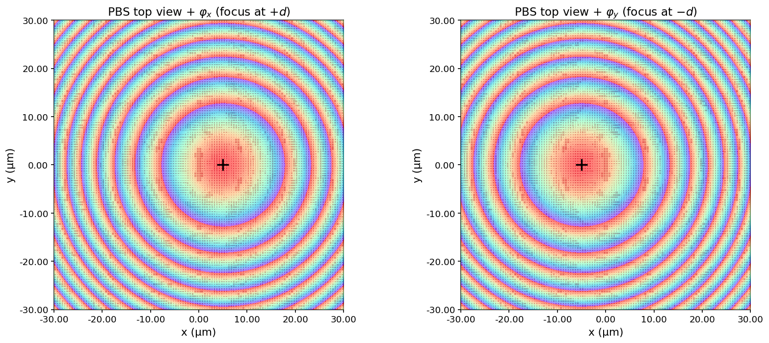
$$ \varphi_x(x,y) \;=\; -\frac{2\pi}{\lambda}\!\left(\sqrt{(x - d)^2 + y^2 + f^2} - f\right) \pmod{2\pi} $$
$$ \varphi_y(x,y) \;=\; -\frac{2\pi}{\lambda}\!\left(\sqrt{(x + d)^2 + y^2 + f^2} - f\right) \pmod{2\pi} $$
x-polarized light is focused to $(+d, 0)$ where an x-meander is placed, and y-polarized light is focused to $(-d, 0)$ where a y-meander is placed. Varying d trades off lateral spot separation against spot quality, which directly sets the polarization cross-talk.
8.1 Pre-Computed PBS Meta-Atom Library¶
We sample $\varphi_x \times \varphi_y$ on an 8 × 8 grid of 45° bins (64 combinations) and pick one $(\ell_x, \ell_y)$ pair per bin from a pre-computed unit-cell library. The two arrays LX and LY below store these dimensions, indexed by 1 + bin_x*8 + bin_y (index 0 is a placeholder).
The taller meta-atoms (h_ant = 1.96 µm) are needed to reach 2π phase coverage with anisotropic shapes.
# --- PBS-specific geometry ---
H_ANT_PBS    = 1.96
CAVITY_H_PBS = 0.233
CELL_PBS     = 0.5
NUM_CELLS_PBS = int(L_METALENS / CELL_PBS)

# 8x8 anisotropic meta-atom library (indexed by 1 + 8*bin_x + bin_y)
LX = np.array([0,
    0.238, 0.220, 0.220, 0.210, 0.206, 0.206, 0.273, 0.248,
    0.248, 0.248, 0.234, 0.227, 0.227, 0.213, 0.298, 0.266,
    0.266, 0.259, 0.345, 0.425, 0.302, 0.386, 0.309, 0.287,
    0.298, 0.284, 0.386, 0.266, 0.450, 0.263, 0.355, 0.316,
    0.252, 0.248, 0.425, 0.241, 0.280, 0.351, 0.294, 0.355,
    0.337, 0.100, 0.100, 0.446, 0.294, 0.153, 0.128, 0.118,
    0.160, 0.153, 0.153, 0.149, 0.142, 0.210, 0.408, 0.174,
    0.195, 0.188, 0.188, 0.178, 0.171, 0.263, 0.224, 0.210,
])
LY = np.array([0,
    0.238, 0.259, 0.270, 0.302, 0.323, 0.337, 0.160, 0.195,
    0.227, 0.248, 0.256, 0.294, 0.280, 0.333, 0.153, 0.192,
    0.224, 0.234, 0.345, 0.234, 0.425, 0.100, 0.153, 0.189,
    0.210, 0.231, 0.323, 0.266, 0.227, 0.298, 0.139, 0.178,
    0.369, 0.390, 0.302, 0.439, 0.280, 0.418, 0.245, 0.171,
    0.206, 0.369, 0.386, 0.319, 0.273, 0.146, 0.220, 0.263,
    0.270, 0.302, 0.309, 0.316, 0.386, 0.132, 0.404, 0.224,
    0.245, 0.291, 0.273, 0.319, 0.355, 0.118, 0.174, 0.210,
])


def pbs_atom_size(phi_x_deg, phi_y_deg):
    """Return (lx, ly) for the meta-atom at the given (φ_x, φ_y) bin pair."""
    bx = int(phi_x_deg // 45)
    by = int(phi_y_deg // 45)
    if not (0 <= bx < 8 and 0 <= by < 8):
        return None
    idx = 1 + bx*8 + by
    return float(LX[idx]), float(LY[idx])


def pbs_meta_atoms(L, na, d, cell_size, num_cells, lda,
                   sub_z, sub_t, h_ant):
    """
    Build the list of rectangular meta-atoms for a PBS metasurface that focuses
    x-pol to (+d, 0) and y-pol to (-d, 0).
    """
    f00 = (L/2) / np.tan(np.arcsin(na))
    xc = np.linspace(-L/2 + cell_size/2, L/2 - cell_size/2, num_cells)
    yc = np.linspace(-L/2 + cell_size/2, L/2 - cell_size/2, num_cells)

    atoms = []
    for x in xc:
        for y in yc:
            phi_x = np.mod((-2*np.pi/lda *
                            (np.sqrt((x - d)**2 + y**2 + f00**2) - f00)) * 180/np.pi,
                           360)
            phi_y = np.mod((-2*np.pi/lda *
                            (np.sqrt((x + d)**2 + y**2 + f00**2) - f00)) * 180/np.pi,
                           360)
            sizes = pbs_atom_size(phi_x, phi_y)
            if sizes is None:
                continue
            sx, sy = sizes
            atoms.append(td.Box(
                center=[x, y, sub_z + sub_t/2 + h_ant/2],
                size=[sx, sy, h_ant],
            ))
    return atoms, f00
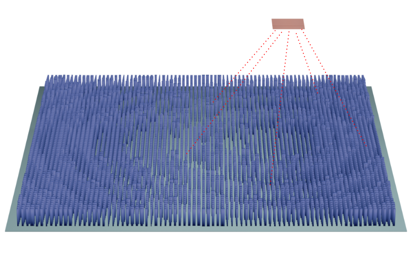
9. PBS Top-View Visualization¶
We visualize the PBS metasurface at $d = 5$ µm, showing the rectangular meta-atoms (top) with each of the two designed phase profiles $\varphi_x$ and $\varphi_y$ overlaid. Note how $\varphi_x$ is a hyperbolic phase centered at $(+d, 0)$ (marked with a black cross), and $\varphi_y$ at $(-d, 0)$.
NA_PBS = 0.5
D_VIZ  = 5.0

# Build a minimal dummy simulation just so we can use `sim.plot_structures`
f00_pbs = (L_METALENS/2) / np.tan(np.arcsin(NA_PBS))
f_pbs   = f00_pbs - H_ANT_PBS - 5.0          # match build_pbs_sim() default offset

L_sim_xy_pbs = L_METALENS + 2 * XY_BUFFER
L_h_pbs      = 2*LDA/3 + SUB_T + H_ANT_PBS + f_pbs + CAVITY_H_PBS
sub_z_pbs    = -L_h_pbs/2 + 2*LDA/3 + SUB_T/2
mid_z_pbs    = sub_z_pbs + SUB_T/2 + H_ANT_PBS/2

metalens_sub_pbs = td.Structure(
    geometry=td.Box(center=[0, 0, sub_z_pbs],
                    size=[td.inf, td.inf, SUB_T]),
    name="metalens_sub", medium=SIO2,
)
atoms_viz, _ = pbs_meta_atoms(L_METALENS, NA_PBS, D_VIZ,
                              CELL_PBS, NUM_CELLS_PBS, LDA,
                              sub_z=sub_z_pbs, sub_t=SUB_T, h_ant=H_ANT_PBS)
metalens_pbs_viz = td.Structure(
    geometry=td.GeometryGroup(geometries=atoms_viz),
    medium=SILICON, name="metalens",
)

dummy_sim = td.Simulation(
    size=(L_sim_xy_pbs, L_sim_xy_pbs, L_h_pbs),
    grid_spec=td.GridSpec.auto(wavelength=LDA, min_steps_per_wvl=6),
    structures=[metalens_sub_pbs, metalens_pbs_viz],
    boundary_spec=td.BoundarySpec(
        x=td.Boundary.pml(), y=td.Boundary.pml(),
        z=td.Boundary(minus=td.PML(), plus=td.PECBoundary()),
    ),
    sources=[td.PlaneWave(
        name="dummy", center=[0, 0, sub_z_pbs - SUB_T],
        size=[L_METALENS, L_METALENS, 0],
        source_time=td.GaussianPulse(freq0=F0, fwidth=F0/5),
        direction="+",
    )],
    monitors=[],
    run_time=1e-14,
)

# Phase profiles
xs = np.linspace(-L_METALENS/2, L_METALENS/2, 600)
ys = np.linspace(-L_METALENS/2, L_METALENS/2, 600)
X, Y = np.meshgrid(xs, ys, indexing="xy")
phi_x = np.mod(-2*np.pi/LDA *
               (np.sqrt((X - D_VIZ)**2 + Y**2 + f00_pbs**2) - f00_pbs), 2*np.pi)
phi_y = np.mod(-2*np.pi/LDA *
               (np.sqrt((X + D_VIZ)**2 + Y**2 + f00_pbs**2) - f00_pbs), 2*np.pi)

def darken_small_patches(ax, max_dim=1.0):
    for p in ax.patches:
        try:
            w, h = p.get_width(), p.get_height()
            if max(abs(w), abs(h)) < max_dim:
                p.set_facecolor("black")
                p.set_edgecolor("none")
        except AttributeError:
            pass

fig, axes = plt.subplots(1, 2, figsize=(14, 6))
extent = [-L_METALENS/2, L_METALENS/2, -L_METALENS/2, L_METALENS/2]

for ax, phi_field, d_sign in [(axes[0], phi_x, +1), (axes[1], phi_y, -1)]:
    dummy_sim.plot_structures(z=mid_z_pbs, ax=ax)
    darken_small_patches(ax)
    ax.imshow(phi_field, origin="lower", extent=extent,
              cmap="rainbow", vmin=0, vmax=2*np.pi,
              alpha=0.55, aspect="equal", zorder=10)
    ax.plot(d_sign*D_VIZ, 0, "k+", markersize=14, markeredgewidth=2, zorder=11)
    ax.set_xlim(-L_METALENS/2, L_METALENS/2)
    ax.set_ylim(-L_METALENS/2, L_METALENS/2)
    ax.set_aspect("equal")
    ax.set_xlabel("x (µm)")
    ax.set_ylabel("y (µm)")

axes[0].set_title(rf"PBS top view + $\varphi_x$ (focus at $+d$)")
axes[1].set_title(rf"PBS top view + $\varphi_y$ (focus at $-d$)")

plt.tight_layout()
plt.savefig(os.path.join(FIG_DIR, "pbs_top_view_phase.png"))
plt.show()
print(f"PBS meta-atoms at d = {D_VIZ} µm: {len(atoms_viz)}")
PBS meta-atoms at d = 5.0 µm: 14400
10. PBS Dual-Meander Absorption Sweep¶
For each focal-spot half-separation d, we now run two FDTD simulations: one with an x-polarized source and one with a y-polarized source. The simulation contains both meanders (x-meander at $+d$, y-meander at $-d$) at all times — only the source polarization changes between runs.
This lets us extract, for each d:
- Intended absorption — x-pol → x-meander, y-pol → y-meander
- Unintended absorption — x-pol → y-meander, y-pol → x-meander
- Cross-talk — $\mathrm{CT}_\mathrm{dB} = 10 \log_{10}(P_\mathrm{unintended} / P_\mathrm{intended})$
FlexCredit note: twelve more 3D FDTD simulations (six d values × two polarizations).
D_LIST = np.array([2.6, 3.5, 5.0, 10.0, 15.0, 20.0])


def build_pbs_sim(d, pol, L=L_METALENS, na=NA_PBS, f_offset_pbs=5.0):
    """
    Build an FDTD simulation for the PBS metasurface with both x- and y-meanders.

    `pol` selects which input polarization is excited ('x' or 'y'); the geometry
    is identical between the two cases.

    `f_offset_pbs` is the empirical paraxial-to-actual focal-plane correction
    for the anisotropic PBS meta-atom library at NA = 0.5.
    """
    f00 = (L/2) / np.tan(np.arcsin(na))
    f   = f00 - H_ANT_PBS - f_offset_pbs

    L_sim_xy = L + 2 * XY_BUFFER
    L_h      = 2*LDA/3 + SUB_T + H_ANT_PBS + f + CAVITY_H_PBS
    sub_z    = -L_h/2 + 2*LDA/3 + SUB_T/2
    metalens_top = sub_z + SUB_T/2 + H_ANT_PBS
    cavity_z = metalens_top + f + CAVITY_H_PBS/2
    cavity_bot = cavity_z - CAVITY_H_PBS/2
    nanowire_z = cavity_bot - NW_T/2

    # --- Structures ---
    metalens_sub = td.Structure(
        geometry=td.Box(center=[0, 0, sub_z],
                        size=[td.inf, td.inf, SUB_T]),
        name="metalens_sub", medium=SIO2,
    )
    atoms, _ = pbs_meta_atoms(L, na, d, CELL_PBS, NUM_CELLS_PBS, LDA,
                              sub_z=sub_z, sub_t=SUB_T, h_ant=H_ANT_PBS)
    metalens = td.Structure(
        geometry=td.GeometryGroup(geometries=atoms),
        medium=SILICON, name="metalens",
    )
    cavity = td.Structure(
        geometry=td.Box.from_bounds(
            rmin=[-1e5, -1e5, cavity_bot],
            rmax=[ 1e5,  1e5,  1e5],
        ),
        name="cavity", medium=SIO2,
    )

    # --- Two meanders ---
    nw_y0_x = -(2*NW_N - 1)*NW_W/2 + NW_W/2                  # x-meander wires shift in y
    x_wires = [
        td.Box(center=[d, nw_y0_x + 2*NW_W*n, nanowire_z],
               size=[NW_L, NW_W, NW_T])
        for n in range(NW_N)
    ]
    nw_y0_y = -d - (2*NW_N - 1)*NW_W/2 + NW_W/2              # y-meander wires shift in x
    y_wires = [
        td.Box(center=[nw_y0_y + 2*NW_W*n, 0, nanowire_z],
               size=[NW_W, NW_L, NW_T])
        for n in range(NW_N)
    ]
    x_meander = td.Structure(
        geometry=td.GeometryGroup(geometries=x_wires),
        medium=NBTIN, name="x_meander",
    )
    y_meander = td.Structure(
        geometry=td.GeometryGroup(geometries=y_wires),
        medium=NBTIN, name="y_meander",
    )

    # --- Source ---
    src = td.PlaneWave(
        name=f"{pol}_pol",
        center=[0, 0, sub_z - SUB_T],
        size=[L, L, 0],
        source_time=td.GaussianPulse(freq0=F0, fwidth=F0/5),
        num_freqs=1, direction="+",
        pol_angle=0 if pol == "x" else np.pi/2,
    )

    # --- Field monitors over each meander volume ---
    nw_total = (2*NW_N - 1)*NW_W + 2*0.02
    abs_mon_x = td.FieldMonitor(
        name="abs_mon_x",
        center=[d, 0, nanowire_z],
        size=[NW_L, nw_total, NW_T + 0.02],
        freqs=[F0], fields=["Ex", "Ey", "Ez"],
    )
    abs_mon_y = td.FieldMonitor(
        name="abs_mon_y",
        center=[-d, 0, nanowire_z],
        size=[nw_total, NW_L, NW_T + 0.02],
        freqs=[F0], fields=["Ex", "Ey", "Ez"],
    )
    focal_field = td.FieldMonitor(
        name="focal_field",
        center=[0, 0, nanowire_z],
        size=[td.inf, td.inf, 0],
        freqs=[F0], fields=["Ex", "Ey", "Ez"],
    )
    field_xz = td.FieldMonitor(
        name="field_xz",
        size=[td.inf, 0, td.inf],
        freqs=[F0], fields=["Ex", "Ey", "Ez"],
    )

    # --- Mesh refinement on each meander ---
    refine_x = td.MeshOverrideStructure(
        geometry=td.Box(center=[d, 0, nanowire_z],
                        size=[NW_L, nw_total, NW_T]),
        dl=[None, 0.02, 0.003],
    )
    refine_y = td.MeshOverrideStructure(
        geometry=td.Box(center=[-d, 0, nanowire_z],
                        size=[nw_total, NW_L, NW_T]),
        dl=[0.02, None, 0.003],
    )

    boundary_z = td.Boundary(minus=td.PML(), plus=td.PECBoundary())

    sim = td.Simulation(
        size=(L_sim_xy, L_sim_xy, L_h),
        grid_spec=td.GridSpec.auto(
            wavelength=LDA, min_steps_per_wvl=6,
            override_structures=[refine_x, refine_y],
        ),
        structures=[metalens_sub, metalens, cavity, x_meander, y_meander],
        boundary_spec=td.BoundarySpec(
            x=td.Boundary.pml(), y=td.Boundary.pml(), z=boundary_z,
        ),
        sources=[src],
        monitors=[abs_mon_x, abs_mon_y, focal_field, field_xz],
        run_time=5e-13,
    )
    return sim, dict(n_atoms=len(atoms), nanowire_z=nanowire_z, L_h=L_h)


# --- Launch the sweep ---
for d in D_LIST:
    print(f"\n######  d = {d:.2f} µm  ######")
    for pol in ("x", "y"):
        sim, info = build_pbs_sim(d, pol)
        print(f"  [{pol}-pol]  meta-atoms = {info['n_atoms']},  L_h = {info['L_h']:.2f} µm")
        web.run(
            sim,
            task_name=f"pol_split_d{d:.2f}_{pol}",
            path=os.path.join(DATA_DIR, f"pol_split_d{d:.2f}_{pol}.hdf5"),
            verbose=True,
        )

print("\nAll PBS sweep runs complete.")
######  d = 2.60 µm  ######
  [x-pol]  meta-atoms = 14400,  L_h = 48.33 µm
16:26:56 -03 Created task 'pol_split_d2.60_x' with resource_id
             'fdve-6ed03c93-c245-4931-9723-ae91530b0e11' and task_type 'FDTD'.
             View task using web UI at
             'https://tidy3d.simulation.cloud/workbench?taskId=fdve-6ed03c93-c24
             5-4931-9723-ae91530b0e11'.
Task folder: 'default'.
Output()
16:27:03 -03 Estimated FlexCredit cost: 4.978. Minimum cost depends on task
             execution details. Use 'web.real_cost(task_id)' to get the billed
             FlexCredit cost after a simulation run.
16:27:05 -03 status = queued
             To cancel the simulation, use 'web.abort(task_id)' or
             'web.delete(task_id)' or abort/delete the task in the web UI.
             Terminating the Python script will not stop the job running on the
             cloud.
Output()
16:27:20 -03 status = preprocess
16:27:26 -03 starting up solver
running solver
Output()
16:34:26 -03 status = postprocess
Output()
16:34:32 -03 status = success
16:34:34 -03 View simulation result at
             'https://tidy3d.simulation.cloud/workbench?taskId=fdve-6ed03c93-c24
             5-4931-9723-ae91530b0e11'.
Output()
16:34:51 -03 Loading results from data/pol_split_d2.60_x.hdf5
16:34:52 -03 WARNING: Simulation final field decay value of 0.0701 is greater
             than the simulation shutoff threshold of 1e-05. Consider running
             the simulation again with a larger 'run_time' duration for more
             accurate results.
[y-pol] meta-atoms = 14400, L_h = 48.33 µm
16:34:55 -03 Created task 'pol_split_d2.60_y' with resource_id
             'fdve-b6b3cdb2-6d0d-416d-b5ed-7e2f8f475285' and task_type 'FDTD'.
             View task using web UI at
             'https://tidy3d.simulation.cloud/workbench?taskId=fdve-b6b3cdb2-6d0
             d-416d-b5ed-7e2f8f475285'.
Task folder: 'default'.
Output()
16:35:01 -03 Estimated FlexCredit cost: 4.978. Minimum cost depends on task
             execution details. Use 'web.real_cost(task_id)' to get the billed
             FlexCredit cost after a simulation run.
16:35:03 -03 status = queued
             To cancel the simulation, use 'web.abort(task_id)' or
             'web.delete(task_id)' or abort/delete the task in the web UI.
             Terminating the Python script will not stop the job running on the
             cloud.
Output()
16:35:16 -03 status = preprocess
16:35:25 -03 starting up solver
running solver
Output()
16:42:40 -03 status = postprocess
Output()
16:42:47 -03 status = success
16:42:49 -03 View simulation result at
             'https://tidy3d.simulation.cloud/workbench?taskId=fdve-b6b3cdb2-6d0
             d-416d-b5ed-7e2f8f475285'.
Output()
16:43:08 -03 Loading results from data/pol_split_d2.60_y.hdf5
16:43:09 -03 WARNING: Simulation final field decay value of 0.0821 is greater
             than the simulation shutoff threshold of 1e-05. Consider running
             the simulation again with a larger 'run_time' duration for more
             accurate results.
######  d = 3.50 µm  ######
  [x-pol]  meta-atoms = 14400,  L_h = 48.33 µm
16:43:12 -03 Created task 'pol_split_d3.50_x' with resource_id
             'fdve-9c02c923-54bf-42d0-aba1-840d98e7a151' and task_type 'FDTD'.
             View task using web UI at
             'https://tidy3d.simulation.cloud/workbench?taskId=fdve-9c02c923-54b
             f-42d0-aba1-840d98e7a151'.
Task folder: 'default'.
Output()
16:43:19 -03 Estimated FlexCredit cost: 4.971. Minimum cost depends on task execution details. Use 'web.real_cost(task_id)' to get the billed FlexCredit cost after a simulation run.
16:43:21 -03 status = queued
To cancel the simulation, use 'web.abort(task_id)' or 'web.delete(task_id)' or abort/delete the task in the web UI. Terminating the Python script will not stop the job running on the cloud.
Output()
16:43:31 -03 status = preprocess
16:43:48 -03 starting up solver
running solver
Output()
16:45:02 -03 status = postprocess
Output()
16:45:09 -03 status = success
16:45:11 -03 View simulation result at 'https://tidy3d.simulation.cloud/workbench?taskId=fdve-9c02c923-54b f-42d0-aba1-840d98e7a151'.
Output()
16:45:29 -03 Loading results from data/pol_split_d3.50_x.hdf5
16:45:30 -03 WARNING: Simulation final field decay value of 0.0742 is greater than the simulation shutoff threshold of 1e-05. Consider running the simulation again with a larger 'run_time' duration for more accurate results.
[y-pol] meta-atoms = 14400, L_h = 48.33 µm
16:45:33 -03 Created task 'pol_split_d3.50_y' with resource_id 'fdve-efa6efe9-8eea-4cb1-8374-772700aa2247' and task_type 'FDTD'.
View task using web UI at 'https://tidy3d.simulation.cloud/workbench?taskId=fdve-efa6efe9-8ee a-4cb1-8374-772700aa2247'.
Task folder: 'default'.
Output()
16:45:39 -03 Estimated FlexCredit cost: 4.971. Minimum cost depends on task execution details. Use 'web.real_cost(task_id)' to get the billed FlexCredit cost after a simulation run.
16:45:42 -03 status = queued
To cancel the simulation, use 'web.abort(task_id)' or 'web.delete(task_id)' or abort/delete the task in the web UI. Terminating the Python script will not stop the job running on the cloud.
Output()
16:46:22 -03 status = preprocess
16:46:31 -03 starting up solver
running solver
Output()
16:50:00 -03 status = postprocess
Output()
16:50:06 -03 status = success
16:50:08 -03 View simulation result at 'https://tidy3d.simulation.cloud/workbench?taskId=fdve-efa6efe9-8ee a-4cb1-8374-772700aa2247'.
Output()
16:50:15 -03 Loading results from data/pol_split_d3.50_y.hdf5
16:50:16 -03 WARNING: Simulation final field decay value of 0.0834 is greater than the simulation shutoff threshold of 1e-05. Consider running the simulation again with a larger 'run_time' duration for more accurate results.
###### d = 5.00 µm ###### [x-pol] meta-atoms = 14400, L_h = 48.33 µm
16:50:18 -03 Created task 'pol_split_d5.00_x' with resource_id 'fdve-b7784f58-6559-46f4-a47b-30131e4d5ad7' and task_type 'FDTD'.
View task using web UI at 'https://tidy3d.simulation.cloud/workbench?taskId=fdve-b7784f58-655 9-46f4-a47b-30131e4d5ad7'.
Task folder: 'default'.
Output()
16:50:26 -03 Estimated FlexCredit cost: 4.975. Minimum cost depends on task execution details. Use 'web.real_cost(task_id)' to get the billed FlexCredit cost after a simulation run.
16:50:28 -03 status = queued
To cancel the simulation, use 'web.abort(task_id)' or 'web.delete(task_id)' or abort/delete the task in the web UI. Terminating the Python script will not stop the job running on the cloud.
Output()
16:50:44 -03 status = preprocess
16:50:55 -03 starting up solver
16:50:56 -03 running solver
Output()
16:54:26 -03 status = postprocess
Output()
16:54:32 -03 status = success
16:54:34 -03 View simulation result at 'https://tidy3d.simulation.cloud/workbench?taskId=fdve-b7784f58-655 9-46f4-a47b-30131e4d5ad7'.
Output()
16:54:41 -03 Loading results from data/pol_split_d5.00_x.hdf5
16:54:42 -03 WARNING: Simulation final field decay value of 0.0755 is greater than the simulation shutoff threshold of 1e-05. Consider running the simulation again with a larger 'run_time' duration for more accurate results.
[y-pol] meta-atoms = 14400, L_h = 48.33 µm
16:54:44 -03 Created task 'pol_split_d5.00_y' with resource_id 'fdve-a222347b-d28b-4b55-a257-310dcbf5bff7' and task_type 'FDTD'.
View task using web UI at 'https://tidy3d.simulation.cloud/workbench?taskId=fdve-a222347b-d28 b-4b55-a257-310dcbf5bff7'.
Task folder: 'default'.
Output()
16:54:51 -03 Estimated FlexCredit cost: 4.975. Minimum cost depends on task execution details. Use 'web.real_cost(task_id)' to get the billed FlexCredit cost after a simulation run.
16:54:53 -03 status = queued
To cancel the simulation, use 'web.abort(task_id)' or 'web.delete(task_id)' or abort/delete the task in the web UI. Terminating the Python script will not stop the job running on the cloud.
Output()
16:55:11 -03 status = preprocess
16:55:20 -03 starting up solver
running solver
Output()
17:02:13 -03 status = postprocess
Output()
17:02:20 -03 status = success
17:02:22 -03 View simulation result at 'https://tidy3d.simulation.cloud/workbench?taskId=fdve-a222347b-d28 b-4b55-a257-310dcbf5bff7'.
Output()
17:02:30 -03 Loading results from data/pol_split_d5.00_y.hdf5
17:02:31 -03 WARNING: Simulation final field decay value of 0.0852 is greater than the simulation shutoff threshold of 1e-05. Consider running the simulation again with a larger 'run_time' duration for more accurate results.
###### d = 10.00 µm ###### [x-pol] meta-atoms = 14400, L_h = 48.33 µm
17:02:33 -03 Created task 'pol_split_d10.00_x' with resource_id 'fdve-fef42b68-200b-4acb-b12c-ec2b535efb51' and task_type 'FDTD'.
View task using web UI at 'https://tidy3d.simulation.cloud/workbench?taskId=fdve-fef42b68-200 b-4acb-b12c-ec2b535efb51'.
Task folder: 'default'.
Output()
17:02:39 -03 Estimated FlexCredit cost: 4.971. Minimum cost depends on task execution details. Use 'web.real_cost(task_id)' to get the billed FlexCredit cost after a simulation run.
17:02:42 -03 status = queued
To cancel the simulation, use 'web.abort(task_id)' or 'web.delete(task_id)' or abort/delete the task in the web UI. Terminating the Python script will not stop the job running on the cloud.
Output()
17:02:54 -03 status = preprocess
17:03:05 -03 starting up solver
17:03:06 -03 running solver
Output()
17:05:54 -03 status = postprocess
Output()
17:06:04 -03 status = success
17:06:06 -03 View simulation result at 'https://tidy3d.simulation.cloud/workbench?taskId=fdve-fef42b68-200 b-4acb-b12c-ec2b535efb51'.
Output()
17:06:17 -03 Loading results from data/pol_split_d10.00_x.hdf5
17:06:18 -03 WARNING: Simulation final field decay value of 0.0768 is greater than the simulation shutoff threshold of 1e-05. Consider running the simulation again with a larger 'run_time' duration for more accurate results.
[y-pol] meta-atoms = 14400, L_h = 48.33 µm
17:06:20 -03 Created task 'pol_split_d10.00_y' with resource_id 'fdve-8ced7ba0-2f96-4812-9151-d1d05dbcfaea' and task_type 'FDTD'.
View task using web UI at 'https://tidy3d.simulation.cloud/workbench?taskId=fdve-8ced7ba0-2f9 6-4812-9151-d1d05dbcfaea'.
Task folder: 'default'.
Output()
17:06:26 -03 Estimated FlexCredit cost: 4.971. Minimum cost depends on task execution details. Use 'web.real_cost(task_id)' to get the billed FlexCredit cost after a simulation run.
17:06:29 -03 status = queued
To cancel the simulation, use 'web.abort(task_id)' or 'web.delete(task_id)' or abort/delete the task in the web UI. Terminating the Python script will not stop the job running on the cloud.
Output()
17:06:41 -03 status = preprocess
17:06:52 -03 starting up solver
17:06:53 -03 running solver
Output()
17:09:43 -03 status = postprocess
Output()
17:09:50 -03 status = success
17:09:52 -03 View simulation result at 'https://tidy3d.simulation.cloud/workbench?taskId=fdve-8ced7ba0-2f9 6-4812-9151-d1d05dbcfaea'.
Output()
17:10:10 -03 Loading results from data/pol_split_d10.00_y.hdf5
WARNING: Simulation final field decay value of 0.0868 is greater than the simulation shutoff threshold of 1e-05. Consider running the simulation again with a larger 'run_time' duration for more accurate results.
###### d = 15.00 µm ###### [x-pol] meta-atoms = 14400, L_h = 48.33 µm
17:10:13 -03 Created task 'pol_split_d15.00_x' with resource_id 'fdve-2fe92977-9da9-4da1-b7e6-ccd4069d3df1' and task_type 'FDTD'.
View task using web UI at 'https://tidy3d.simulation.cloud/workbench?taskId=fdve-2fe92977-9da 9-4da1-b7e6-ccd4069d3df1'.
Task folder: 'default'.
Output()
17:10:20 -03 Estimated FlexCredit cost: 4.971. Minimum cost depends on task execution details. Use 'web.real_cost(task_id)' to get the billed FlexCredit cost after a simulation run.
17:10:22 -03 status = queued
To cancel the simulation, use 'web.abort(task_id)' or 'web.delete(task_id)' or abort/delete the task in the web UI. Terminating the Python script will not stop the job running on the cloud.
Output()
17:10:34 -03 status = preprocess
17:10:39 -03 starting up solver
17:10:40 -03 running solver
Output()
17:17:40 -03 status = postprocess
Output()
17:17:47 -03 status = success
17:17:49 -03 View simulation result at 'https://tidy3d.simulation.cloud/workbench?taskId=fdve-2fe92977-9da 9-4da1-b7e6-ccd4069d3df1'.
Output()
17:18:04 -03 Loading results from data/pol_split_d15.00_x.hdf5
17:18:05 -03 WARNING: Simulation final field decay value of 0.0782 is greater than the simulation shutoff threshold of 1e-05. Consider running the simulation again with a larger 'run_time' duration for more accurate results.
[y-pol] meta-atoms = 14400, L_h = 48.33 µm
17:18:08 -03 Created task 'pol_split_d15.00_y' with resource_id 'fdve-bc3db93b-ea76-4796-80d9-bb6654d067c4' and task_type 'FDTD'.
View task using web UI at 'https://tidy3d.simulation.cloud/workbench?taskId=fdve-bc3db93b-ea7 6-4796-80d9-bb6654d067c4'.
Task folder: 'default'.
Output()
17:18:15 -03 Estimated FlexCredit cost: 4.971. Minimum cost depends on task execution details. Use 'web.real_cost(task_id)' to get the billed FlexCredit cost after a simulation run.
17:18:17 -03 status = queued
To cancel the simulation, use 'web.abort(task_id)' or 'web.delete(task_id)' or abort/delete the task in the web UI. Terminating the Python script will not stop the job running on the cloud.
Output()
17:18:30 -03 status = preprocess
17:18:38 -03 starting up solver
running solver
Output()
17:25:47 -03 status = postprocess
Output()
17:25:53 -03 status = success
17:25:55 -03 View simulation result at 'https://tidy3d.simulation.cloud/workbench?taskId=fdve-bc3db93b-ea7 6-4796-80d9-bb6654d067c4'.
Output()
17:26:28 -03 Loading results from data/pol_split_d15.00_y.hdf5
17:26:29 -03 WARNING: Simulation final field decay value of 0.0893 is greater than the simulation shutoff threshold of 1e-05. Consider running the simulation again with a larger 'run_time' duration for more accurate results.
###### d = 20.00 µm ###### [x-pol] meta-atoms = 14400, L_h = 48.33 µm
17:26:32 -03 Created task 'pol_split_d20.00_x' with resource_id 'fdve-9f76c500-f053-4d4d-a0b4-ecb57cdbe476' and task_type 'FDTD'.
View task using web UI at 'https://tidy3d.simulation.cloud/workbench?taskId=fdve-9f76c500-f05 3-4d4d-a0b4-ecb57cdbe476'.
Task folder: 'default'.
Output()
17:26:39 -03 Estimated FlexCredit cost: 4.967. Minimum cost depends on task execution details. Use 'web.real_cost(task_id)' to get the billed FlexCredit cost after a simulation run.
17:26:41 -03 status = queued
To cancel the simulation, use 'web.abort(task_id)' or 'web.delete(task_id)' or abort/delete the task in the web UI. Terminating the Python script will not stop the job running on the cloud.
Output()
17:27:00 -03 status = preprocess
17:27:07 -03 starting up solver
17:27:08 -03 running solver
Output()
17:33:54 -03 status = postprocess
Output()
17:34:01 -03 status = success
17:34:03 -03 View simulation result at 'https://tidy3d.simulation.cloud/workbench?taskId=fdve-9f76c500-f05 3-4d4d-a0b4-ecb57cdbe476'.
Output()
17:34:30 -03 Loading results from data/pol_split_d20.00_x.hdf5
17:34:31 -03 WARNING: Simulation final field decay value of 0.0785 is greater than the simulation shutoff threshold of 1e-05. Consider running the simulation again with a larger 'run_time' duration for more accurate results.
[y-pol] meta-atoms = 14400, L_h = 48.33 µm
17:34:34 -03 Created task 'pol_split_d20.00_y' with resource_id 'fdve-07bb7172-6a61-4e9c-89f8-e40e21ab6afb' and task_type 'FDTD'.
View task using web UI at 'https://tidy3d.simulation.cloud/workbench?taskId=fdve-07bb7172-6a6 1-4e9c-89f8-e40e21ab6afb'.
Task folder: 'default'.
Output()
17:34:40 -03 Estimated FlexCredit cost: 4.967. Minimum cost depends on task execution details. Use 'web.real_cost(task_id)' to get the billed FlexCredit cost after a simulation run.
17:34:43 -03 status = queued
To cancel the simulation, use 'web.abort(task_id)' or 'web.delete(task_id)' or abort/delete the task in the web UI. Terminating the Python script will not stop the job running on the cloud.
Output()
17:34:55 -03 status = preprocess
17:35:06 -03 starting up solver
17:35:07 -03 running solver
Output()
17:37:55 -03 status = postprocess
Output()
17:38:07 -03 status = success
17:38:09 -03 View simulation result at 'https://tidy3d.simulation.cloud/workbench?taskId=fdve-07bb7172-6a6 1-4e9c-89f8-e40e21ab6afb'.
Output()
17:38:20 -03 Loading results from data/pol_split_d20.00_y.hdf5
17:38:21 -03 WARNING: Simulation final field decay value of 0.0886 is greater than the simulation shutoff threshold of 1e-05. Consider running the simulation again with a larger 'run_time' duration for more accurate results.
All PBS sweep runs complete.
11. PBS Post-Processing — Cross-Talk vs Separation¶
Same idea as Section 6 — we integrate $\tfrac{1}{2}\sigma|E|^2$ over the NbTiN volume — but now we have two meanders and two input polarizations, so we extract four absorbed-power numbers per d. From those we compute the cross-talk in dB.
MON_X = "abs_mon_x"
MON_Y = "abs_mon_y"
def absorbed_power(monitor_data, nanowire_z, axis, d):
"""
P_abs = ½σ ∫∫∫ |E|² dV over the NbTiN volume of one meander.
The monitor stores a box that lightly over-bounds the meander; we mask
along all three axes to integrate only over the actual wire strands.
"""
Ex = monitor_data.Ex.abs.isel(f=0).squeeze(drop=True)
Ey = monitor_data.Ey.abs.isel(f=0).squeeze(drop=True)
Ez = monitor_data.Ez.abs.isel(f=0).squeeze(drop=True)
E2 = Ex**2 + Ey**2 + Ez**2
xs = E2.coords["x"].values
ys = E2.coords["y"].values
zs = E2.coords["z"].values
mask_z = (zs >= nanowire_z - NW_T/2) & (zs <= nanowire_z + NW_T/2)
if axis == "x":
nw_y0 = -(2*NW_N - 1)*NW_W/2 + NW_W/2
mask_x = (xs >= d - NW_L/2) & (xs <= d + NW_L/2)
mask_y = np.zeros_like(ys, dtype=bool)
for n in range(NW_N):
yc = nw_y0 + 2*NW_W*n
mask_y |= (ys >= yc - NW_W/2) & (ys <= yc + NW_W/2)
else:
nw_x0 = -d - (2*NW_N - 1)*NW_W/2 + NW_W/2
mask_y = (ys >= -NW_L/2) & (ys <= NW_L/2)
mask_x = np.zeros_like(xs, dtype=bool)
for n in range(NW_N):
xc = nw_x0 + 2*NW_W*n
mask_x |= (xs >= xc - NW_W/2) & (xs <= xc + NW_W/2)
mask = (xr.DataArray(mask_x.astype(float), coords=[("x", xs)])
* xr.DataArray(mask_y.astype(float), coords=[("y", ys)])
* xr.DataArray(mask_z.astype(float), coords=[("z", zs)]))
integrand = E2 * mask
P = (0.5 * NBTIN_SIGMA * integrand
.integrate(coord="x")
.integrate(coord="y")
.integrate(coord="z"))
return float(P.values)
rows = []
for d in D_LIST:
row = {"d_um": float(d)}
print(f"===== d = {d:.2f} µm =====")
for pol in ("x", "y"):
path = os.path.join(DATA_DIR, f"pol_split_d{d:.2f}_{pol}.hdf5")
if not os.path.exists(path):
print(f" [skip] {path}")
for k in ("Pabs_x", "Pabs_y", "intended", "unintended", "crosstalk_dB"):
row[f"{k}_{pol}"] = np.nan
continue
sd = td.SimulationData.from_file(path)
nw_z = sd.simulation.get_monitor_by_name(MON_X).center[2]
P_x = absorbed_power(sd[MON_X], nw_z, axis="x", d=d)
P_y = absorbed_power(sd[MON_Y], nw_z, axis="y", d=d)
intended = P_x if pol == "x" else P_y
unintended = P_y if pol == "x" else P_x
ct_dB = (10 * np.log10(unintended / intended)
if (intended > 0 and unintended > 0) else np.nan)
row[f"Pabs_x_{pol}"] = P_x
row[f"Pabs_y_{pol}"] = P_y
row[f"intended_{pol}"] = intended
row[f"unintended_{pol}"] = unintended
row[f"crosstalk_dB_{pol}"] = ct_dB
print(f" [{pol}-pol] P_abs(x-mnd) = {P_x*100:6.3f} %"
f" P_abs(y-mnd) = {P_y*100:6.3f} %"
f" CT = {ct_dB:6.2f} dB")
rows.append(row)
df_pbs = pd.DataFrame(rows)
csv_path = os.path.join(DATA_DIR, "pbs_summary.csv")
df_pbs.to_csv(csv_path, index=False)
print(f"\nSaved: {csv_path}")
df_pbs
===== d = 2.60 µm ===== [x-pol] P_abs(x-mnd) = 47.627 % P_abs(y-mnd) = 4.277 % CT = -10.47 dB [y-pol] P_abs(x-mnd) = 1.293 % P_abs(y-mnd) = 35.510 % CT = -14.39 dB ===== d = 3.50 µm ===== [x-pol] P_abs(x-mnd) = 47.640 % P_abs(y-mnd) = 1.597 % CT = -14.75 dB [y-pol] P_abs(x-mnd) = 0.509 % P_abs(y-mnd) = 35.951 % CT = -18.49 dB ===== d = 5.00 µm ===== [x-pol] P_abs(x-mnd) = 47.050 % P_abs(y-mnd) = 1.467 % CT = -15.06 dB [y-pol] P_abs(x-mnd) = 0.511 % P_abs(y-mnd) = 34.364 % CT = -18.28 dB ===== d = 10.00 µm ===== [x-pol] P_abs(x-mnd) = 46.368 % P_abs(y-mnd) = 1.246 % CT = -15.71 dB [y-pol] P_abs(x-mnd) = 0.701 % P_abs(y-mnd) = 32.687 % CT = -16.69 dB ===== d = 15.00 µm ===== [x-pol] P_abs(x-mnd) = 45.006 % P_abs(y-mnd) = 1.652 % CT = -14.35 dB [y-pol] P_abs(x-mnd) = 0.864 % P_abs(y-mnd) = 32.366 % CT = -15.73 dB ===== d = 20.00 µm ===== [x-pol] P_abs(x-mnd) = 41.900 % P_abs(y-mnd) = 1.629 % CT = -14.10 dB [y-pol] P_abs(x-mnd) = 0.622 % P_abs(y-mnd) = 29.364 % CT = -16.74 dB Saved: data/pbs_summary.csv
| d_um | Pabs_x_x | Pabs_y_x | intended_x | unintended_x | crosstalk_dB_x | Pabs_x_y | Pabs_y_y | intended_y | unintended_y | crosstalk_dB_y | |
|---|---|---|---|---|---|---|---|---|---|---|---|
| 0 | 2.6 | 0.476272 | 0.042772 | 0.476272 | 0.042772 | -10.466974 | 0.012926 | 0.355096 | 0.355096 | 0.012926 | -14.388930 |
| 1 | 3.5 | 0.476399 | 0.015975 | 0.476399 | 0.015975 | -14.745411 | 0.005091 | 0.359512 | 0.359512 | 0.005091 | -18.489409 |
| 2 | 5.0 | 0.470502 | 0.014675 | 0.470502 | 0.014675 | -15.059945 | 0.005112 | 0.343636 | 0.343636 | 0.005112 | -18.275019 |
| 3 | 10.0 | 0.463682 | 0.012460 | 0.463682 | 0.012460 | -15.707041 | 0.007012 | 0.326873 | 0.326873 | 0.007012 | -16.685366 |
| 4 | 15.0 | 0.450061 | 0.016516 | 0.450061 | 0.016516 | -14.353584 | 0.008643 | 0.323660 | 0.323660 | 0.008643 | -15.734438 |
| 5 | 20.0 | 0.418997 | 0.016285 | 0.418997 | 0.016285 | -14.104188 | 0.006224 | 0.293639 | 0.293639 | 0.006224 | -16.737599 |
11.1 Plots — Intended/Unintended Absorption and Cross-Talk vs d¶
# --- Plot 1: intended (left axis) + unintended (right axis, 0-5%) ---
fig, ax_L = plt.subplots(figsize=(7.5, 5))
l1, = ax_L.plot(df_pbs["d_um"], df_pbs["intended_x"]*100,
"o-", color="C0", lw=2, ms=8,
label=r"x-pol $\to$ x-meander (intended)")
l2, = ax_L.plot(df_pbs["d_um"], df_pbs["intended_y"]*100,
"^-", color="C3", lw=2, ms=8,
label=r"y-pol $\to$ y-meander (intended)")
ax_L.set_xlabel("Focal-spot half-separation d (µm)")
ax_L.set_ylabel("Intended-port absorption (% of input)")
ax_L.grid(alpha=0.3)
ax_R = ax_L.twinx()
l3, = ax_R.plot(df_pbs["d_um"], df_pbs["unintended_x"]*100,
"s--", color="C0", lw=1.5, ms=7, alpha=0.7,
label=r"x-pol $\to$ y-meander (unintended)")
l4, = ax_R.plot(df_pbs["d_um"], df_pbs["unintended_y"]*100,
"v--", color="C3", lw=1.5, ms=7, alpha=0.7,
label=r"y-pol $\to$ x-meander (unintended)")
ax_R.set_ylabel("Unintended-port absorption (% of input)")
ax_R.set_ylim(0, 5)
ax_L.legend(handles=[l1, l2, l3, l4], loc="best", frameon=False)
plt.title("Intended- and unintended-port absorption vs separation")
plt.tight_layout()
plt.savefig(os.path.join(FIG_DIR, "pbs_absorption_vs_d.png"))
plt.show()
# --- Plot 2: cross-talk (dB) ---
fig, ax = plt.subplots(figsize=(7, 5))
ax.plot(df_pbs["d_um"], df_pbs["crosstalk_dB_x"],
"o-", color="C0", lw=2, ms=8, label="x-pol input")
ax.plot(df_pbs["d_um"], df_pbs["crosstalk_dB_y"],
"^-", color="C3", lw=2, ms=8, label="y-pol input")
ax.set_xlabel("Focal-spot half-separation d (µm)")
ax.set_ylabel(r"Cross-talk $10\log_{10}(P_\mathrm{unint.}/P_\mathrm{int.})$ (dB)")
ax.set_title("Polarization cross-talk vs nanowire separation")
ax.legend(loc="best", frameon=False)
ax.grid(alpha=0.3)
plt.tight_layout()
plt.savefig(os.path.join(FIG_DIR, "pbs_crosstalk_vs_d.png"))
plt.show()
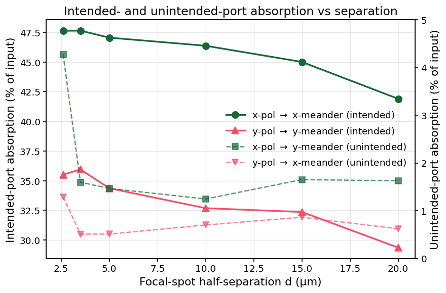
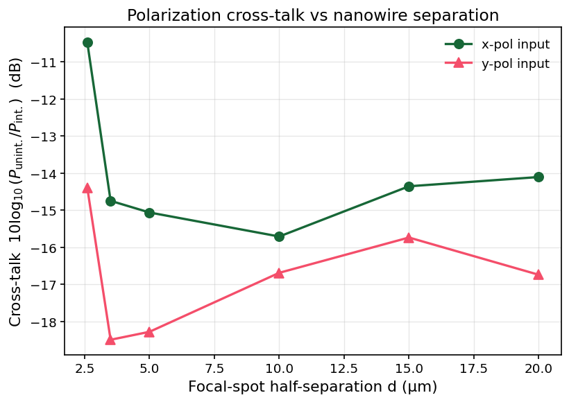
12. PBS Field-Distribution Heatmaps (d = 5 µm)¶
For one representative separation we plot $|E|^2$ in two orthogonal cuts — the xz cross-section (top row) and the focal plane (bottom row) — under x- and y-polarized excitation. This visually confirms that each polarization is steered to the correct meander.
D_HM = 5.0
XZ_MON = "field_xz"
FOCAL_MON = "focal_field"
VMIN, VMAX = 0, 100
AXIS_LIM = (-30, 30)
def E2_from(monitor):
Ex = monitor.Ex.abs.isel(f=0).squeeze(drop=True)
Ey = monitor.Ey.abs.isel(f=0).squeeze(drop=True)
Ez = monitor.Ez.abs.isel(f=0).squeeze(drop=True)
return Ex**2 + Ey**2 + Ez**2
def _add_cbar(im, ax):
div = make_axes_locatable(ax)
cax = div.append_axes("right", size="4%", pad=0.08)
cbar = ax.figure.colorbar(im, cax=cax)
cbar.set_label(r"$|E|^2$ (arb. units)")
cbar.outline.set_linewidth(0.6)
def plot_heatmap(ax, sd, mon_name, b_label, title):
E2 = E2_from(sd[mon_name])
coords = list(E2.coords)
a_name, b_name = coords[0], coords[1]
a = E2.coords[a_name].values
b = E2.coords[b_name].values
Z = E2.values
# Rotate 180° so the source side is at the bottom of the xz panels
Z_rot = Z[::-1, ::-1]
a_rot = -a[::-1]
b_rot = -b[::-1]
im = ax.pcolormesh(a_rot, b_rot, Z_rot.T,
shading="auto", cmap="magma",
vmin=VMIN, vmax=VMAX, rasterized=True)
ax.set_xlim(*AXIS_LIM); ax.set_ylim(*AXIS_LIM)
ax.set_aspect("equal", adjustable="box")
ax.set_xlabel("x (µm)"); ax.set_ylabel(f"{b_label} (µm)")
ax.set_title(title, loc="left", pad=8, fontweight="bold")
_add_cbar(im, ax)
def _load(pol):
path = os.path.join(DATA_DIR, f"pol_split_d{D_HM:.2f}_{pol}.hdf5")
if not os.path.exists(path):
print(f"[skip] {path}")
return None
return td.SimulationData.from_file(path)
sd_x = _load("x")
sd_y = _load("y")
if sd_x is None or sd_y is None:
raise SystemExit("Missing simulation files for d = 5 µm heatmaps.")
fig, axes = plt.subplots(2, 2, figsize=(13, 11))
plot_heatmap(axes[0, 0], sd_x, XZ_MON, "z", "a) xz plane, x-pol")
plot_heatmap(axes[0, 1], sd_y, XZ_MON, "z", "b) xz plane, y-pol")
plot_heatmap(axes[1, 0], sd_x, FOCAL_MON, "y", "c) focal plane, x-pol")
plot_heatmap(axes[1, 1], sd_y, FOCAL_MON, "y", "d) focal plane, y-pol")
plt.tight_layout()
plt.savefig(os.path.join(FIG_DIR, "pbs_4panel_heatmaps.png"))
plt.show()
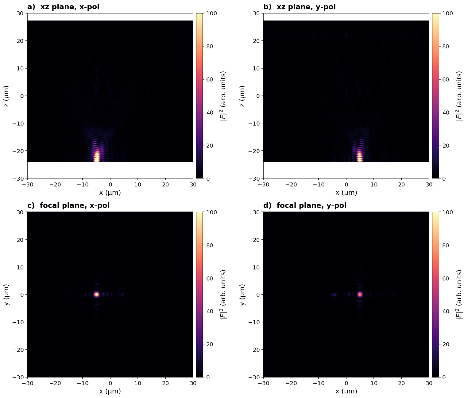
13. Conclusions¶
Two complementary cryogenic dielectric metasurfaces are designed, simulated, and characterized in Tidy3D:
- The focusing metalens (Sections 2–7) concentrates a 60 × 60 µm² collection aperture onto a 5 × 5 µm² nanowire footprint. The component efficiencies $\tilde\eta_c$ (coupling) and $\tilde\eta_a$ (absorption-given-arrival) trade off across NA, with the SDE enhancement factor $A_M/A_D \cdot \eta_\mathrm{abs}$ peaking around the moderate-NA regime.
- The PBS metasurface (Sections 8–12) uses anisotropic rectangular meta-atoms to focus orthogonal linear polarizations onto two separated meanders. Increasing the focal-spot half-separation
dreduces polarization cross-talk monotonically.
Both designs use the same Tidy3D building blocks — GeometryGroup, MeshOverrideStructure for sub-nm nanowire resolution, and a PECBoundary on the top z-face to model the back-reflector cavity. The post-processing routines extract absorbed power directly from the field monitors via the loss-tangent formula $P_\mathrm{abs} = \tfrac{1}{2}\sigma\int|E|^2 dV$.
For experimental validation and fabrication details, see arXiv:2512.17115.