





Author: Amgad A. Salama, ADC RC
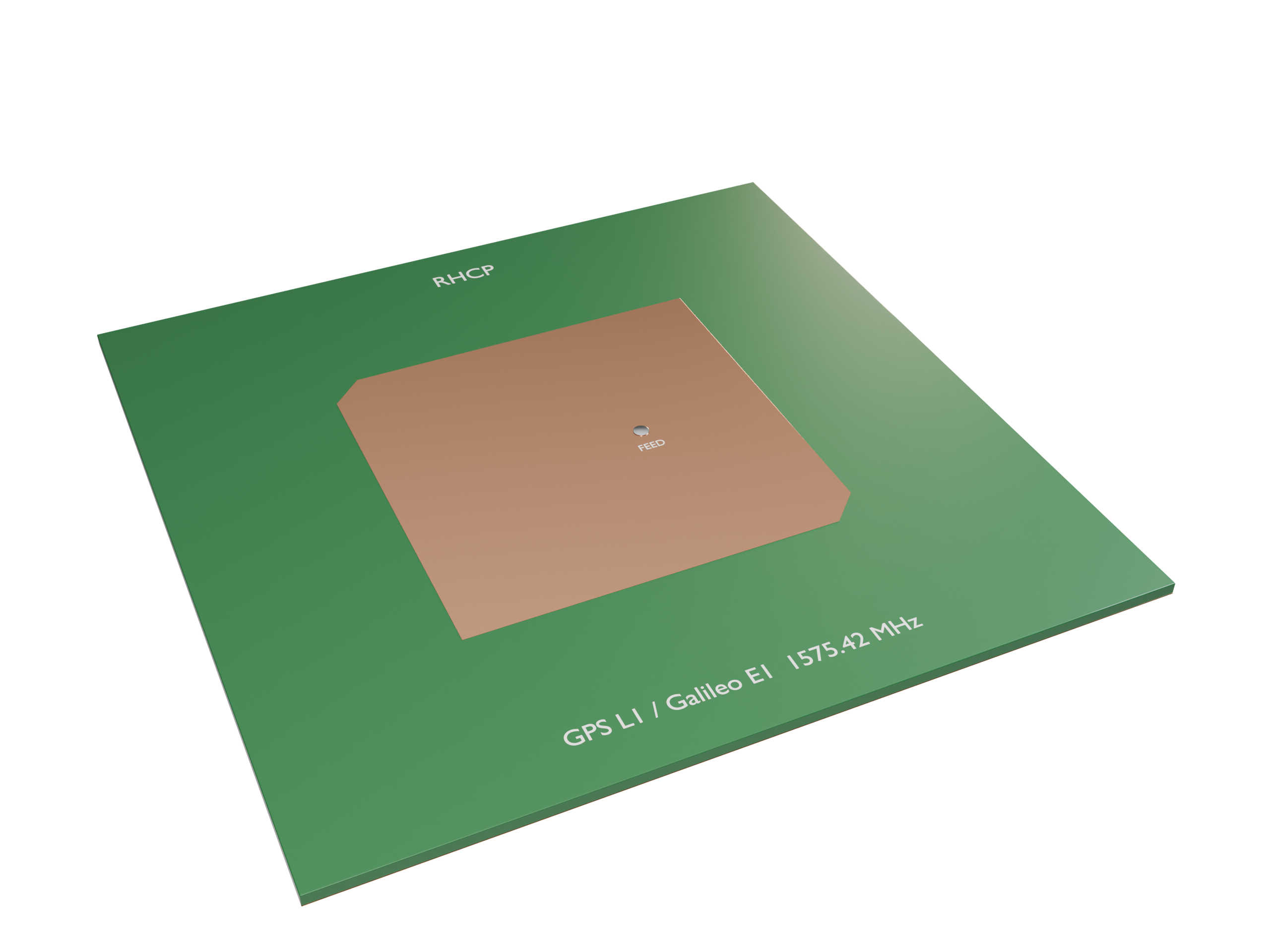
GNSS receivers (GPS, Galileo, BeiDou, GLONASS) need an antenna that receives right-hand circular polarization (RHCP) over almost the whole upper hemisphere. The most common low-cost choice is a single-feed, corner-truncated square microstrip patch, which you can find in many GPS modules, drones and vehicle trackers.
This notebook designs and simulates such an antenna for the GPS L1 / Galileo E1 band (1575.42 MHz) on a Rogers RO4003C substrate. It covers:
- Why GNSS uses RHCP, and what axial ratio means
- An analytical first-pass design: patch size, corner truncation, feed position
- Building the model in Tidy3D with a coaxial probe feed (
CoaxialLumpedPort) and theTerminalComponentModeler - Post-processing: $S_{11}$, input impedance, the rotating near field, RHCP/LHCP realized gain, and axial ratio vs. frequency and elevation
- A parametric sweep showing how corner truncation trades impedance match against circular polarization
Design targets
| Quantity | Target |
|---|---|
| Center frequency | 1575.42 MHz (GPS L1 C/A, Galileo E1) |
| Polarization | RHCP |
| $S_{11}$ at $f_0$ | < −10 dB |
| Axial ratio at boresight | < 3 dB |
| RHCP realized gain at boresight | ≳ 5 dBic |
1. Background: Why Circular Polarization?
GNSS satellites transmit RHCP signals. Circular polarization is used for two reasons:
- Faraday rotation. The ionosphere rotates a linear polarization by an unknown angle. A CP wave is unaffected by this rotation.
- Multipath rejection. When an RHCP wave reflects once off the ground or a building, its handedness flips to LHCP. An antenna that receives RHCP well and LHCP poorly suppresses these reflected signals, which are a major source of positioning error.
Axial ratio (AR). In general, the field vector traces an ellipse. AR is the ratio of its major axis to its minor axis: 0 dB is perfect circular polarization and ∞ is linear. The usual specification is AR < 3 dB. Equivalently, the cross-polarized (LHCP) gain is related to AR by
$$\frac{|E_{LHCP}|}{|E_{RHCP}|} = \frac{AR-1}{AR+1}, \qquad AR = 3\text{ dB} \;\Rightarrow\; \text{XPD} \approx 15\text{ dB}.$$
How a single feed makes CP. A square patch supports two orthogonal, degenerate modes ($TM_{010}$ and $TM_{001}$). Cutting off two opposite corners makes the patch slightly shorter along that diagonal. This splits the two diagonal modes into a higher frequency $f_a$ and a lower frequency $f_b$. A feed on the $x$-axis excites both diagonal modes equally. Between $f_b$ and $f_a$:
- the higher mode (below its resonance) is capacitive, so its phase leads by about 45°
- the lower mode (above its resonance) is inductive, so its phase lags by about 45°
The two modes are then 90° apart in phase with equal amplitude, which gives circular polarization. Which pair of corners is cut sets the handedness. With the feed on the $+x$ axis, cutting the $(+x,-y)$ and $(-x,+y)$ corners gives RHCP toward $+z$. Mirroring the cut gives LHCP. We check this in the simulation results.
import matplotlib.pyplot as plt
import numpy as np
import tidy3d as td
from tidy3d import (
    rf,  # RF components: CoaxialLumpedPort, TerminalComponentModeler
    web,
)

print("Tidy3D version:", td.__version__)  # written and validated against 2.12

# Tidy3D's length unit is the micrometer; work in mm for readability
mm = 1e3
c0 = td.C_0
Tidy3D version: 2.12.0
2. Analytical First-Pass Design
2.1 Substrate and Frequency Band
We use Rogers RO4003C, 1.524 mm (60 mil) thick, with $\varepsilon_r = 3.55$ (the design value) and $\tan\delta = 0.0027$. The simulation covers 1.45 to 1.70 GHz. Around $f_0$ we also sample a fine set of frequencies (2 MHz step) at which the far fields are recorded.
f0 = 1.57542e9  # GPS L1 / Galileo E1
fmin, fmax = 1.45e9, 1.70e9
lam0 = c0 / f0

# frequencies where the far field is recorded (must be a subset of the S-parameter freqs)
f_rad = f0 + np.arange(-20, 21) * 2e6
freqs = np.unique(np.concatenate([np.linspace(fmin, fmax, 126), f_rad]))

eps_r, tan_d = 3.55, 0.0027
h = 1.524 * mm  # substrate thickness
print(f"free-space wavelength at f0: {lam0 / mm:.1f} mm")
free-space wavelength at f0: 190.3 mm
2.2 Patch Size (Transmission-Line Model)
For a square patch ($W = L$), the fringing fields make the patch look electrically longer by $\Delta L$ at each radiating edge:
$$\varepsilon_{\text{eff}} = \frac{\varepsilon_r+1}{2} + \frac{\varepsilon_r-1}{2}\left(1+12\frac{h}{W}\right)^{-1/2},\qquad \frac{\Delta L}{h} = 0.412\,\frac{(\varepsilon_{\text{eff}}+0.3)(W/h+0.264)}{(\varepsilon_{\text{eff}}-0.258)(W/h+0.8)},$$
$$L = \frac{c_0}{2 f_0\sqrt{\varepsilon_{\text{eff}}}} - 2\Delta L .$$
$W = L$ here, so we iterate until the result stops changing.
L = c0 / (2 * f0 * np.sqrt(eps_r))  # initial guess
for _ in range(20):
    eps_eff = (eps_r + 1) / 2 + (eps_r - 1) / 2 / np.sqrt(1 + 12 * h / L)
    dL = (
        0.412
        * h
        * (eps_eff + 0.3)
        * (L / h + 0.264)
        / ((eps_eff - 0.258) * (L / h + 0.8))
    )
    L = c0 / (2 * f0 * np.sqrt(eps_eff)) - 2 * dL

print(
    f"eps_eff = {eps_eff:.3f},  dL = {dL / mm:.3f} mm,  patch side L = {L / mm:.2f} mm"
)
eps_eff = 3.367, dL = 0.729 mm, patch side L = 50.39 mm
2.3 Corner Truncation
The size of the two removed triangles controls how far apart the two modes are. The classic design rule (Sharma & Gupta, 1983) relates the removed area $\Delta S$ to the unloaded quality factor $Q_0$ of the patch:
$$\frac{\Delta S}{S} \approx \frac{1}{2Q_0}, \qquad \Delta S = 2\cdot\tfrac{1}{2}c^2 = c^2 \;\Rightarrow\; c = \frac{L}{\sqrt{2Q_0}}$$
where $c$ is the leg length of each triangle cut from a corner. We estimate $Q_0$ from the radiation Q (Jackson & Alexopoulos closed form) and the dielectric Q, $Q_d = 1/\tan\delta$. Conductor loss is much smaller than either and is neglected.
c1 = 1 - 1 / eps_r + 2 / (5 * eps_r**2)
Q_rad = 3 * eps_r / (16 * c1) * lam0 / h  # square patch, L/W = 1
Q_d = 1 / tan_d
Q0 = 1 / (1 / Q_rad + 1 / Q_d)
cut = L / np.sqrt(2 * Q0)
print(f"Q_rad ~ {Q_rad:.0f},  Q_d ~ {Q_d:.0f},  Q0 ~ {Q0:.0f}")
print(f"corner truncation leg c ~ {cut / mm:.2f} mm")
print(
    f"expected CP fractional bandwidth ~ 1/Q0 ~ {100 / Q0:.1f} %  (AR<3dB is typically much narrower)"
)
Q_rad ~ 111,  Q_d ~ 370,  Q0 ~ 85
corner truncation leg c ~ 3.86 mm
expected CP fractional bandwidth ~ 1/Q0 ~ 1.2 %  (AR<3dB is typically much narrower)
2.4 Feed Position and Coaxial Probe
The input resistance of a probe-fed patch falls from its maximum at the edge to zero at the center, roughly as $\cos^2(\pi x_e/L)$, where $x_e$ is the distance from the radiating edge. For a 60-mil substrate the edge resistance is a few hundred ohms, which puts 50 Ω at about $x_f \approx 0.15L$ from the center. The value is only a starting point: with two modes excited the impedance changes, so we tune $x_f$ later.
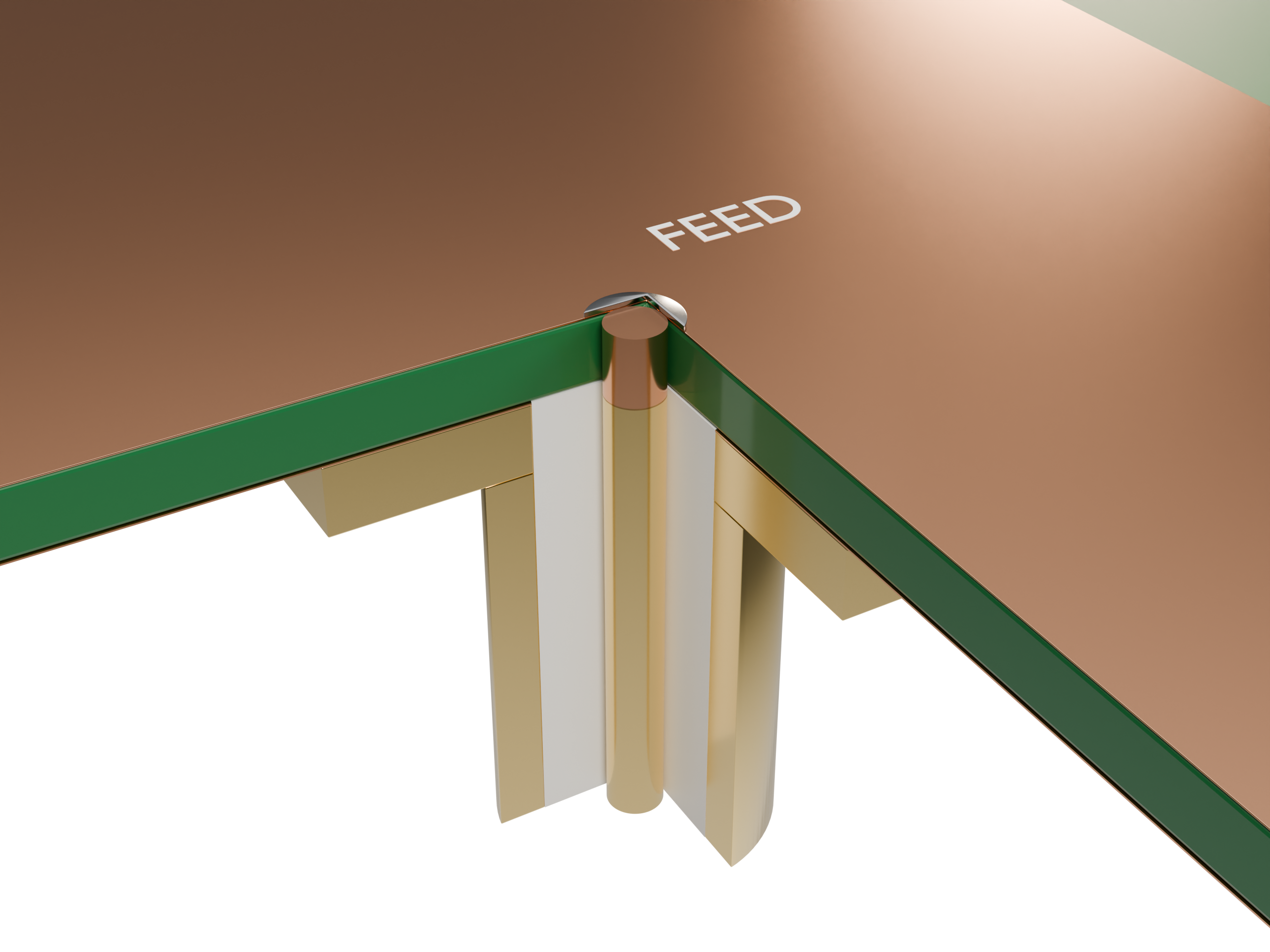
The probe is an SMA-style pin (1.27 mm diameter) inside a 4.1 mm clearance hole in the ground plane. This annulus is where the CoaxialLumpedPort sits.
xf = 0.15 * L  # feed offset from center, along +x
r_in = 0.635 * mm  # probe (inner conductor) radius
r_out = 2.05 * mm  # ground-plane clearance (outer conductor) radius
Lg = 100 * mm  # ground plane side (~0.53 lambda0)

# round analytical values to "manufacturable" numbers for the baseline design
L0, cut0, xf0 = round(L / mm, 1) * mm, round(cut / mm, 1) * mm, round(xf / mm, 1) * mm
print(f"baseline: L = {L0 / mm} mm, c = {cut0 / mm} mm, xf = {xf0 / mm} mm")
baseline: L = 50.4 mm, c = 3.9 mm, xf = 7.6 mm
3. Building the Tidy3D Model
The patch and ground plane are modeled as zero-thickness PEC sheets (td.PEC2D), and the probe as a PEC cylinder. This is the standard approach for printed antennas. Resolving a 35 µm copper layer would force a very small time step, while the conductor loss it adds is small compared to the dielectric loss here.
The function below builds the whole TerminalComponentModeler from three design parameters, so we can reuse it in the parameter sweep.
Meshing notes
-
LayerRefinementSpecputs several cells across the thin substrate and refines the patch corners. - A
MeshOverrideStructuresets about 0.8 mm resolution over the patch, so the mode frequencies converge. - The coaxial port automatically refines the mesh across the annulus (
num_grid_cells). - The PML is placed half a wavelength (at $f_{min}$) away from the ground plane.
Radiation monitor. A DirectivityMonitor surrounds the antenna. It records near fields and projects them to the far field on a $(\theta,\phi)$ grid. The modeler combines this with the port data to give realized gain, i.e. gain including mismatch loss.
substrate_med = td.Medium(
    permittivity=eps_r,
    conductivity=2 * np.pi * f0 * td.EPSILON_0 * eps_r * tan_d,  # loss tangent at f0
    name="RO4003C",
)


def truncated_patch(L, cut, z):
    # Square patch with the (+x,-y) and (-x,+y) corners truncated -> RHCP for a +x feed
    a = L / 2
    verts = [
        (-a, -a),
        (a - cut, -a),
        (a, -a + cut),
        (a, a),
        (-a + cut, a),
        (-a, a - cut),
    ]
    return td.PolySlab(vertices=verts, slab_bounds=(z, z), axis=2)


def make_modeler(L=L0, cut=cut0, xf=xf0, theta_pts=91, phi_pts=73):
    substrate = td.Structure(
        geometry=td.Box(center=(0, 0, h / 2), size=(Lg, Lg, h)),
        medium=substrate_med,
        name="substrate",
    )
    ground_geo = td.Box(center=(0, 0, 0), size=(Lg, Lg, 0)) - td.Cylinder(
        center=(xf, 0, 0), radius=r_out, length=0, axis=2
    )
    ground = td.Structure(geometry=ground_geo, medium=td.PEC2D, name="ground")
    patch = td.Structure(
        geometry=truncated_patch(L, cut, h), medium=td.PEC2D, name="patch"
    )
    probe = td.Structure(
        geometry=td.Cylinder(center=(xf, 0, h / 2), radius=r_in, length=h, axis=2),
        medium=td.PEC,
        name="probe",
    )

    port = rf.CoaxialLumpedPort(
        name="feed",
        center=(xf, 0, 0),
        normal_axis=2,
        direction="+",
        inner_diameter=2 * r_in,
        outer_diameter=2 * r_out,
        impedance=50,
    )

    pad = c0 / fmin / 2
    sim_center = (0, 0, h / 2)
    sim_size = (Lg + 2 * pad, Lg + 2 * pad, h + 2 * pad)

    layer_ref = td.LayerRefinementSpec(
        axis=2,
        center=(0, 0, h / 2),
        size=(Lg, Lg, h),
        min_steps_along_axis=4,
        corner_refinement=td.GridRefinement(dl=0.4 * mm, num_cells=2),
    )
    patch_override = td.MeshOverrideStructure(
        geometry=td.Box(center=(0, 0, h / 2), size=(L + 4 * mm, L + 4 * mm, h)),
        dl=(0.8 * mm, 0.8 * mm, None),
    )
    grid_spec = td.GridSpec.auto(
        min_steps_per_wvl=30,
        wavelength=c0 / fmax,
        layer_refinement_specs=[layer_ref],
        override_structures=[patch_override],
    )

    # near field of the dominant mode, recorded in the middle of the substrate
    field_mon = td.FieldMonitor(
        center=(0, 0, h / 2), size=(Lg, Lg, 0), freqs=[f0], fields=["Ez"], name="Ez_mid"
    )

    rad_mon = td.DirectivityMonitor(
        center=sim_center,
        size=(Lg + 20 * mm, Lg + 20 * mm, h + 20 * mm),
        freqs=f_rad,
        theta=np.linspace(0, np.pi, theta_pts),
        phi=np.linspace(0, 2 * np.pi, phi_pts),
        proj_distance=100 * lam0,
        name="radiation",
    )

    sim = td.Simulation(
        center=sim_center,
        size=sim_size,
        grid_spec=grid_spec,
        structures=[substrate, ground, patch, probe],
        monitors=[field_mon],
        boundary_spec=td.BoundarySpec.all_sides(td.PML()),
        run_time=150e-9,  # Q0 ~ 80 -> ring-down ~ Q/(pi f0) ~ 17 ns; field-decay shutoff stops earlier
    )
    return rf.TerminalComponentModeler(
        simulation=sim, ports=[port], freqs=freqs, radiation_monitors=[rad_mon]
    )


modeler = make_modeler()
20:05:32 KST WARNING: RF simulations and functionality will require new license
             requirements in an upcoming release. All RF-specific classes are
             now available within the sub-package 'tidy3d.rf'.
              - Contains monitors defined for RF wavelengths.
             WARNING: 'TerminalComponentModeler' was refactored (tidy3d
             'v2.10.0'). Existing functionality is available differently. Please
             consult the migration documentation:
             https://docs.flexcompute.com/projects/tidy3d/en/latest/api/microwav
             e/microwave_migration.html
3.1 Inspect the Geometry and the Grid
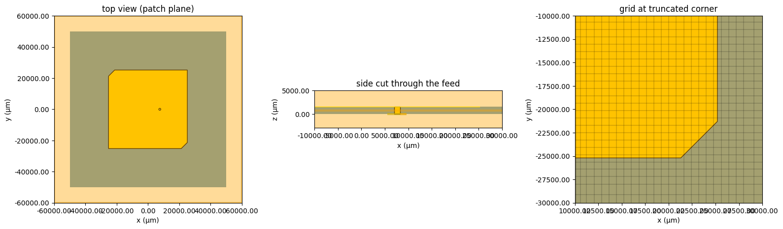
Always check the structure and the mesh before spending FlexCredits. Look for: the truncated corners, the probe passing through the clearance hole, and several grid cells across the substrate.
sim = modeler.base_sim
fig, ax = plt.subplots(1, 3, figsize=(16, 5))
modeler.plot_sim(z=h, ax=ax[0])
ax[0].set_xlim(-60 * mm, 60 * mm)
ax[0].set_ylim(-60 * mm, 60 * mm)
ax[0].set_title("top view (patch plane)")

modeler.plot_sim(y=0, ax=ax[1])
ax[1].set_xlim(-10 * mm, 30 * mm)
ax[1].set_ylim(-3 * mm, 5 * mm)
ax[1].set_title("side cut through the feed")

sim.plot_grid(z=h, ax=ax[2])
sim.plot(z=h, ax=ax[2])
ax[2].set_xlim(10 * mm, 30 * mm)
ax[2].set_ylim(-30 * mm, -10 * mm)
ax[2].set_title("grid at truncated corner")
plt.tight_layout()
plt.show()

print(f"grid: {sim.grid.num_cells}  ->  {sim.num_cells / 1e6:.2f} M cells")
             WARNING: RF simulations and functionality will require new license
             requirements in an upcoming release. All RF-specific classes are
             now available within the sub-package 'tidy3d.rf'.
              - Contains a 'LumpedElement'.
              - Contains monitors defined for RF wavelengths.
grid: [159, 160, 80] -> 2.04 M cells
3.2 Estimate the Cost
job = web.Job(simulation=modeler, task_name="gnss_cp_patch_baseline")
print(f"estimated cost: {job.estimate_cost():.2f} FlexCredits")
             Loading simulation from local cache. View cached task using web UI
             at
             'https://tidy3d.simulation.cloud/rf?taskId=sid-982d69ca-e7c8-4d5e-a
             7ad-e21cc2d1a6ac'.
estimated cost: 0.00 FlexCredits
4. Run the Baseline Design
data = job.run(path="data/gnss_cp_patch_baseline.hdf5")
             WARNING: RF simulations and functionality will require new license
             requirements in an upcoming release. All RF-specific classes are
             now available within the sub-package 'tidy3d.rf'.
              - Contains a 'LumpedElement'.
              - Contains sources defined for RF wavelengths.
              - Contains monitors defined for RF wavelengths.
5. Results
5.1 Reflection Coefficient and Input Impedance
A CP patch has a recognizable impedance signature. The two closely spaced modes produce a small loop (kink) on the Smith chart, and the best CP is usually found near that loop. If $S_{11}$ shows two separate dips, the truncation is too large.
smat = data.smatrix()
s11 = smat.data.isel(port_in=0, port_out=0).squeeze()
f_s = s11.f.values
s11_db = 20 * np.log10(np.abs(s11.values))
z_in = 50 * (1 + s11.values) / (1 - s11.values)

fig, ax = plt.subplots(1, 3, figsize=(17, 4.5))
ax[0].plot(f_s / 1e9, s11_db)
ax[0].axhline(-10, ls="--", c="gray")
ax[0].axvline(f0 / 1e9, ls=":", c="k")
ax[0].set_xlabel("frequency (GHz)")
ax[0].set_ylabel("|S11| (dB)")
ax[0].set_title("Return loss")

ax[1].plot(f_s / 1e9, z_in.real, label="R")
ax[1].plot(f_s / 1e9, z_in.imag, label="X")
ax[1].axhline(50, ls="--", c="gray")
ax[1].axvline(f0 / 1e9, ls=":", c="k")
ax[1].set_xlabel("frequency (GHz)")
ax[1].set_ylabel("Z_in (Ohm)")
ax[1].legend()
ax[1].set_title("Input impedance")

# minimal Smith chart: reflection coefficient in the complex plane
t = np.linspace(0, 2 * np.pi, 200)
ax[2].plot(np.cos(t), np.sin(t), c="gray", lw=0.8)
for r in [0.2, 1, 3]:  # constant-resistance circles
    ax[2].plot(
        r / (1 + r) + np.cos(t) / (1 + r), np.sin(t) / (1 + r), c="lightgray", lw=0.6
    )
ax[2].plot(s11.values.real, s11.values.imag)
i0 = np.argmin(np.abs(f_s - f0))
ax[2].plot(s11.values[i0].real, s11.values[i0].imag, "ro", label="f0")
ax[2].set_aspect("equal")
ax[2].set_xlim(-1.05, 1.05)
ax[2].set_ylim(-1.05, 1.05)
ax[2].legend()
ax[2].set_title("S11 on the Smith chart")
plt.tight_layout()
plt.show()

print(f"|S11| at f0 = {s11_db[i0]:.1f} dB,  Z_in(f0) = {z_in[i0]:.1f} Ohm")
print(f"S11 minimum at {f_s[np.argmin(s11_db)] / 1e9:.4f} GHz")
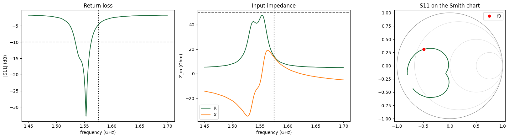
|S11| at f0 = -4.7 dB,  Z_in(f0) = 14.2+13.3j Ohm
S11 minimum at 1.5534 GHz
5.2 Watching the Field Rotate
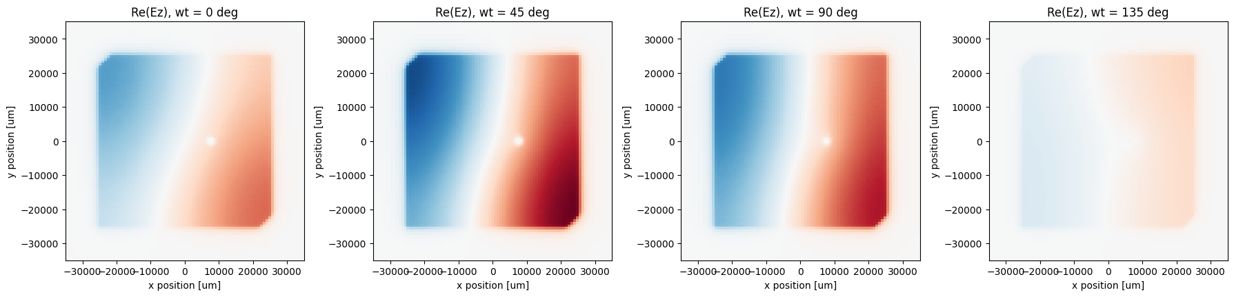
At $f_0$ the field under the patch is a combination of the two diagonal modes, 90° apart in phase. Plotting $\mathrm{Re}\{E_z e^{-i\omega t}\}$ at four instants over a quarter period shows the field pattern rotating around the patch. This is circular polarization visible directly in the near field. The rotation direction you see here matches the handedness of the radiated wave.
sim_data = data.data[modeler.get_task_name(port=modeler.ports[0])]
Ez = sim_data["Ez_mid"].Ez.sel(f=f0, method="nearest").squeeze()

fig, axs = plt.subplots(1, 4, figsize=(18, 4.3))
vmax = np.abs(Ez).max().item()
for ax, ph in zip(axs, [0, 45, 90, 135]):
    # Tidy3D uses the exp(-i w t) convention
    snap = (Ez * np.exp(-1j * np.deg2rad(ph))).real
    snap.plot(
        x="x", y="y", ax=ax, cmap="RdBu_r", vmin=-vmax, vmax=vmax, add_colorbar=False
    )
    ax.set_aspect("equal")
    ax.set_xlim(-35 * mm, 35 * mm)
    ax.set_ylim(-35 * mm, 35 * mm)
    ax.set_title(f"Re(Ez), wt = {ph} deg")
plt.tight_layout()
plt.show()
5.3 Far Field: RHCP/LHCP Gain and Axial Ratio
get_antenna_metrics_data() combines the radiation monitor with the port excitation. We use:
-
partial_realized_gain("circular"), which gives the RHCP (Gright) and LHCP (Gleft) realized gain in dBic. Realized gain includes mismatch loss. -
axial_ratio, the AR as a function of $(\theta, \phi, f)$.
First, AR and gain at boresight ($\theta = 0$) versus frequency. The AR < 3 dB bandwidth of a single-feed patch is narrow, so the AR minimum must sit on $f_0$.
am = data.get_antenna_metrics_data()
G_circ = am.partial_realized_gain("circular")
dB = lambda x: 10 * np.log10(np.maximum(np.asarray(x), 1e-12))
ARdB = lambda x: 20 * np.log10(np.asarray(x))

bs = {"theta": 0, "phi": 0, "method": "nearest"}
f_r = am.f
G_R_bs = dB(G_circ.Gright.sel(**bs).squeeze())
G_L_bs = dB(G_circ.Gleft.sel(**bs).squeeze())
AR_bs = ARdB(am.axial_ratio.sel(**bs).squeeze())

fig, ax = plt.subplots(1, 2, figsize=(13, 4.5))
ax[0].plot(f_r / 1e9, G_R_bs, label="RHCP")
ax[0].plot(f_r / 1e9, G_L_bs, label="LHCP")
ax[0].axvline(f0 / 1e9, ls=":", c="k")
ax[0].set_xlabel("frequency (GHz)")
ax[0].set_ylabel("realized gain (dBic)")
ax[0].legend()
ax[0].set_title("Boresight realized gain")
ax[1].plot(f_r / 1e9, AR_bs)
ax[1].axhline(3, ls="--", c="gray")
ax[1].axvline(f0 / 1e9, ls=":", c="k")
ax[1].set_ylim(0, 15)
ax[1].set_xlabel("frequency (GHz)")
ax[1].set_ylabel("AR (dB)")
ax[1].set_title("Boresight axial ratio")
plt.tight_layout()
plt.show()

i0 = np.argmin(np.abs(f_r - f0))
print(
    f"at f0: RHCP = {G_R_bs[i0]:.2f} dBic, LHCP = {G_L_bs[i0]:.2f} dBic, AR = {AR_bs[i0]:.2f} dB"
)
print(f"AR minimum {AR_bs.min():.2f} dB at {f_r[np.argmin(AR_bs)] / 1e9:.4f} GHz")
ok = AR_bs < 3
if ok.any():
    print(
        f"AR<3dB bandwidth ~ {(f_r[ok].max() - f_r[ok].min()) / 1e6:.0f} MHz (within the sampled +/-40 MHz)"
    )
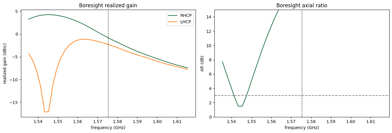
at f0: RHCP = -0.83 dBic, LHCP = -2.29 dBic, AR = 21.53 dB
AR minimum 1.49 dB at 1.5434 GHz
AR<3dB bandwidth ~ 6 MHz (within the sampled +/-40 MHz)
Handedness check: RHCP should exceed LHCP by more than 15 dB at boresight. If LHCP dominates, the cut is on the other diagonal: change the vertex list in
truncated_patchto cut the $(+x,+y)$ and $(-x,-y)$ corners instead. This is also a useful exercise, since mirroring the patch is all it takes to build an LHCP antenna.
5.4 Radiation Patterns at $f_0$
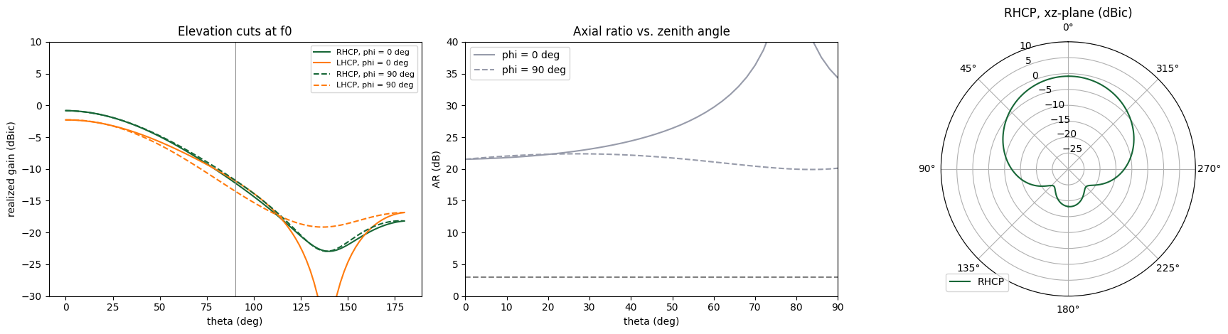
A GNSS antenna has to track satellites down to low elevation (typically a 5°–15° elevation mask, i.e. $\theta$ up to 75°–85°). We plot the pattern in the two principal planes and the AR vs. $\theta$.
theta_deg = np.rad2deg(am.theta)
fig, ax = plt.subplots(1, 3, figsize=(18, 4.8))
for phi_c, ls in [(0, "-"), (np.pi / 2, "--")]:
    sel = {"f": f0, "phi": phi_c, "method": "nearest"}
    lbl = f"phi = {np.rad2deg(phi_c):.0f} deg"
    ax[0].plot(
        theta_deg,
        dB(G_circ.Gright.sel(**sel).squeeze()),
        ls,
        c="C0",
        label=f"RHCP, {lbl}",
    )
    ax[0].plot(
        theta_deg,
        dB(G_circ.Gleft.sel(**sel).squeeze()),
        ls,
        c="C1",
        label=f"LHCP, {lbl}",
    )
    ax[1].plot(
        theta_deg, ARdB(am.axial_ratio.sel(**sel).squeeze()), ls, c="C2", label=lbl
    )
ax[0].set_ylim(-30, 10)
ax[0].set_xlabel("theta (deg)")
ax[0].set_ylabel("realized gain (dBic)")
ax[0].legend(fontsize=8)
ax[0].axvline(90, c="gray", lw=0.6)
ax[0].set_title("Elevation cuts at f0")
ax[1].axhline(3, ls="--", c="gray")
ax[1].set_ylim(0, 40)
ax[1].set_xlim(0, 90)
ax[1].set_xlabel("theta (deg)")
ax[1].set_ylabel("AR (dB)")
ax[1].legend()
ax[1].set_title("Axial ratio vs. zenith angle")

# polar plot (upper hemisphere = theta 0..90) for the phi = 0 cut
ax[2].remove()
axp = fig.add_subplot(1, 3, 3, projection="polar")
g = dB(G_circ.Gright.sel(f=f0, phi=0, method="nearest").squeeze())
g_m = dB(G_circ.Gright.sel(f=f0, phi=np.pi, method="nearest").squeeze())
th = am.theta
axp.plot(th, np.maximum(g, -30), c="C0", label="RHCP")
axp.plot(-th, np.maximum(g_m, -30), c="C0")
axp.set_theta_zero_location("N")
axp.set_rlim(-30, 10)
axp.set_title("RHCP, xz-plane (dBic)")
axp.legend(loc="lower left")
plt.tight_layout()
plt.show()
5.5 3D RHCP Pattern
G3 = (
    G_circ.Gright.sel(f=f0, method="nearest").squeeze().transpose("theta", "phi").values
)
TH, PH = np.meshgrid(am.theta, am.phi, indexing="ij")
Gdb = np.maximum(dB(G3), -20)
R = Gdb + 20  # radial length: gain above a -20 dBic floor
X, Y, Z = R * np.sin(TH) * np.cos(PH), R * np.sin(TH) * np.sin(PH), R * np.cos(TH)

fig = plt.figure(figsize=(7, 6))
ax = fig.add_subplot(projection="3d")
colors = plt.cm.viridis((Gdb - Gdb.min()) / (np.ptp(Gdb) + 1e-9))
ax.plot_surface(
    X, Y, Z, facecolors=colors, rstride=1, cstride=1, linewidth=0, antialiased=False
)
ax.set_box_aspect((1, 1, 1))
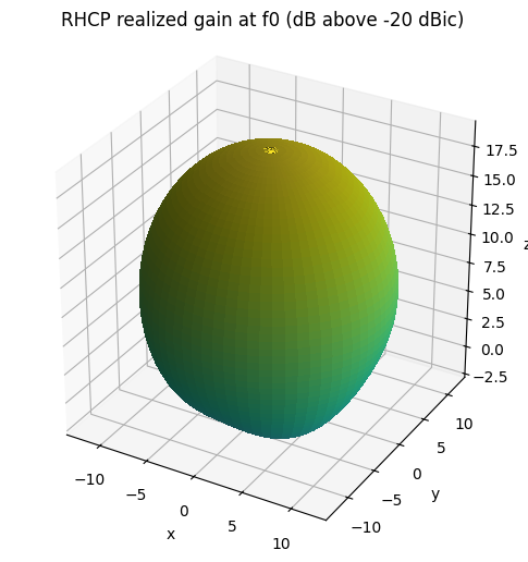
ax.set_title("RHCP realized gain at f0 (dB above -20 dBic)")
ax.set_xlabel("x")
ax.set_ylabel("y")
ax.set_zlabel("z")
plt.show()
6. Design Study: Tuning the Corner Truncation
The analytical rule only gives a starting value. The key tradeoff is:
- truncation too small: the two modes are too close together, the phase difference is below 90°, and the polarization is elliptical (high AR)
- truncation too large: the modes split too far apart, $S_{11}$ shows two dips, and the AR rises again
We sweep $c$ around the analytical value and submit all designs as a single batch. A coarser far-field grid is used to keep the data small. The goal is to find the $c$ that gives the deepest AR minimum, and then to look at the frequency offset between the AR minimum and $f_0$. That offset is corrected by scaling $L$ (a final step left as an exercise).
cuts = np.round(np.array([0.75, 0.875, 1.0, 1.125, 1.25]) * cut0 / mm, 1) * mm
sweep = {
    f"cut_{c / mm:.1f}mm": make_modeler(cut=c, theta_pts=37, phi_pts=37) for c in cuts
}
# cost check before submitting
for name, m in sweep.items():
    print(name, f"{web.Job(simulation=m, task_name=name).estimate_cost():.2f} FC")
20:05:34 KST Loading simulation from local cache. View cached task using web UI
             at
             'https://tidy3d.simulation.cloud/rf?taskId=sid-862c8840-2e9d-444f-b
             3a6-6b16d40ed037'.
cut_2.9mm 0.00 FC
             Loading simulation from local cache. View cached task using web UI
             at
             'https://tidy3d.simulation.cloud/rf?taskId=sid-f9684a5e-0d17-4200-b
             190-ed3d28c1a075'.
cut_3.4mm 0.00 FC
             Loading simulation from local cache. View cached task using web UI
             at
             'https://tidy3d.simulation.cloud/rf?taskId=sid-0764b215-47fc-4362-a
             692-1db127812003'.
cut_3.9mm 0.00 FC
             Loading simulation from local cache. View cached task using web UI
             at
             'https://tidy3d.simulation.cloud/rf?taskId=sid-c0eb3abe-f173-4978-9
             e3e-ac922992c879'.
cut_4.4mm 0.00 FC
             Loading simulation from local cache. View cached task using web UI
             at
             'https://tidy3d.simulation.cloud/rf?taskId=sid-095a931b-bbd4-4163-8
             57e-70e6ac91981a'.
cut_4.9mm 0.00 FC
sweep_data = web.run(sweep, task_name="gnss_cut_sweep", path="data/cut_sweep")
Found all simulations in cache.
fig, ax = plt.subplots(1, 2, figsize=(14, 4.5))
summary = []
for (name, d), c in zip(sweep_data.items(), cuts):
    s = d.smatrix().data.isel(port_in=0, port_out=0).squeeze()
    a = d.get_antenna_metrics_data()
    ar = ARdB(a.axial_ratio.sel(theta=0, phi=0, method="nearest").squeeze())
    ax[0].plot(s.f / 1e9, 20 * np.log10(np.abs(s)), label=f"c = {c / mm:.1f} mm")
    ax[1].plot(a.f / 1e9, ar, label=f"c = {c / mm:.1f} mm")
    summary.append(
        (
            c / mm,
            float(np.min(np.asarray(ar))),
            np.asarray(a.f)[np.argmin(np.asarray(ar))] / 1e9,
            np.asarray(s.f)[np.argmin(np.abs(np.asarray(s)))] / 1e9,
        )
    )
for a_ in ax:
    a_.axvline(f0 / 1e9, ls=":", c="k")
    a_.set_xlabel("frequency (GHz)")
    a_.legend()
ax[0].set_ylabel("|S11| (dB)")
ax[0].set_xlim(1.50, 1.65)
ax[1].set_ylabel("boresight AR (dB)")
ax[1].set_ylim(0, 15)
ax[1].axhline(3, ls="--", c="gray")
plt.tight_layout()
plt.show()

print(" c (mm) | min AR (dB) | f @ min AR (GHz) | f @ min S11 (GHz)")
for row in summary:
    print(
        f"  {row[0]:5.1f} |   {row[1]:6.2f}    |     {row[2]:.4f}       |     {row[3]:.4f}"
    )
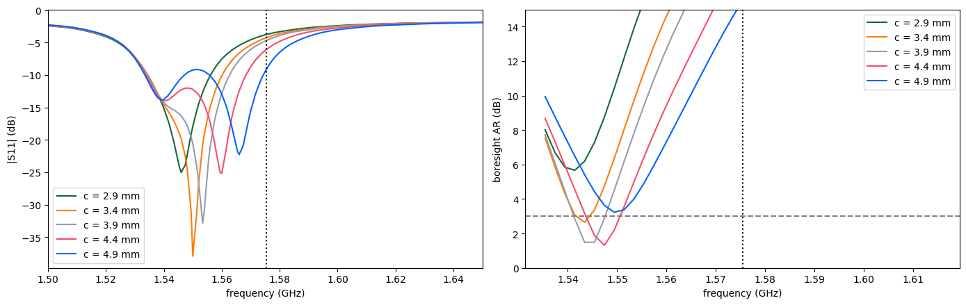
 c (mm) | min AR (dB) | f @ min AR (GHz) | f @ min S11 (GHz)
    2.9 |     5.67    |     1.5414       |     1.5460
    3.4 |     2.65    |     1.5434       |     1.5500
    3.9 |     1.49    |     1.5434       |     1.5534
    4.4 |     1.32    |     1.5474       |     1.5600
    4.9 |     3.23    |     1.5494       |     1.5660
Re-centering the design. Choose the $c$ with the lowest AR minimum and read off the frequency $f_{AR}$ where it occurs. Patch frequencies scale almost inversely with size, so
$$L_{\text{new}} \approx L_0\,\frac{f_{AR}}{f_0}, \qquad c_{\text{new}} \approx c\,\frac{L_{\text{new}}}{L_0}.$$
Rebuild with make_modeler(L=L_new, cut=c_new) and re-run. Then, if needed, adjust xf to bring $|S_{11}|$ at $f_0$ below −10 dB. One or two iterations are usually enough.
7. Takeaways
- A single feed plus a small geometric asymmetry (corner truncation) is enough to produce circular polarization. The price is a narrow AR bandwidth, of order $1/(2Q_0)$, of which the AR < 3 dB region is only a part. That is fine for GPS L1 C/A (±1 MHz) but tight for wider signals such as Galileo E1 (±2 MHz) or L1 P(Y) (±10 MHz).
- Impedance match and CP purity are separate requirements, and they do not peak at the same frequency automatically. Always plot both.
- Use realized gain, not directivity, when comparing designs, because it includes mismatch and dielectric losses.
References
- P. C. Sharma and K. C. Gupta, "Analysis and optimized design of single feed circularly polarized microstrip antennas," IEEE Trans. Antennas Propag., vol. 31, no. 6, 1983.
- D. R. Jackson and N. G. Alexopoulos, "Simple approximate formulas for input resistance, bandwidth, and efficiency of a resonant rectangular patch," IEEE Trans. Antennas Propag., vol. 39, no. 3, 1991.
- R. Garg et al., Microstrip Antenna Design Handbook, Artech House, 2001.


 TERMS & CONDITIONS


 How the process works:
 Try this real URL to see an example: