





Author: Amgad A. Salama, ADC RC
A Butler matrix is a passive, reciprocal $N \times N$ network that turns each of its $N$ input ports into a distinct, fixed beam when its $N$ outputs drive a uniform linear array. Exciting input i produces equal-amplitude outputs with a progressive phase step $\Delta\phi_i$, which steers the main lobe of the array to
$$\sin\theta_i = \frac{\Delta\phi_i}{k_0 d},$$
where $d$ is the element spacing and $k_0 = 2\pi/\lambda_0$. Because it needs no phase shifters, switches or active components in the RF path, the Butler matrix is a classic building block of switched-beam antennas for 5G/Wi-Fi access points, automotive radar and satellite terminals.
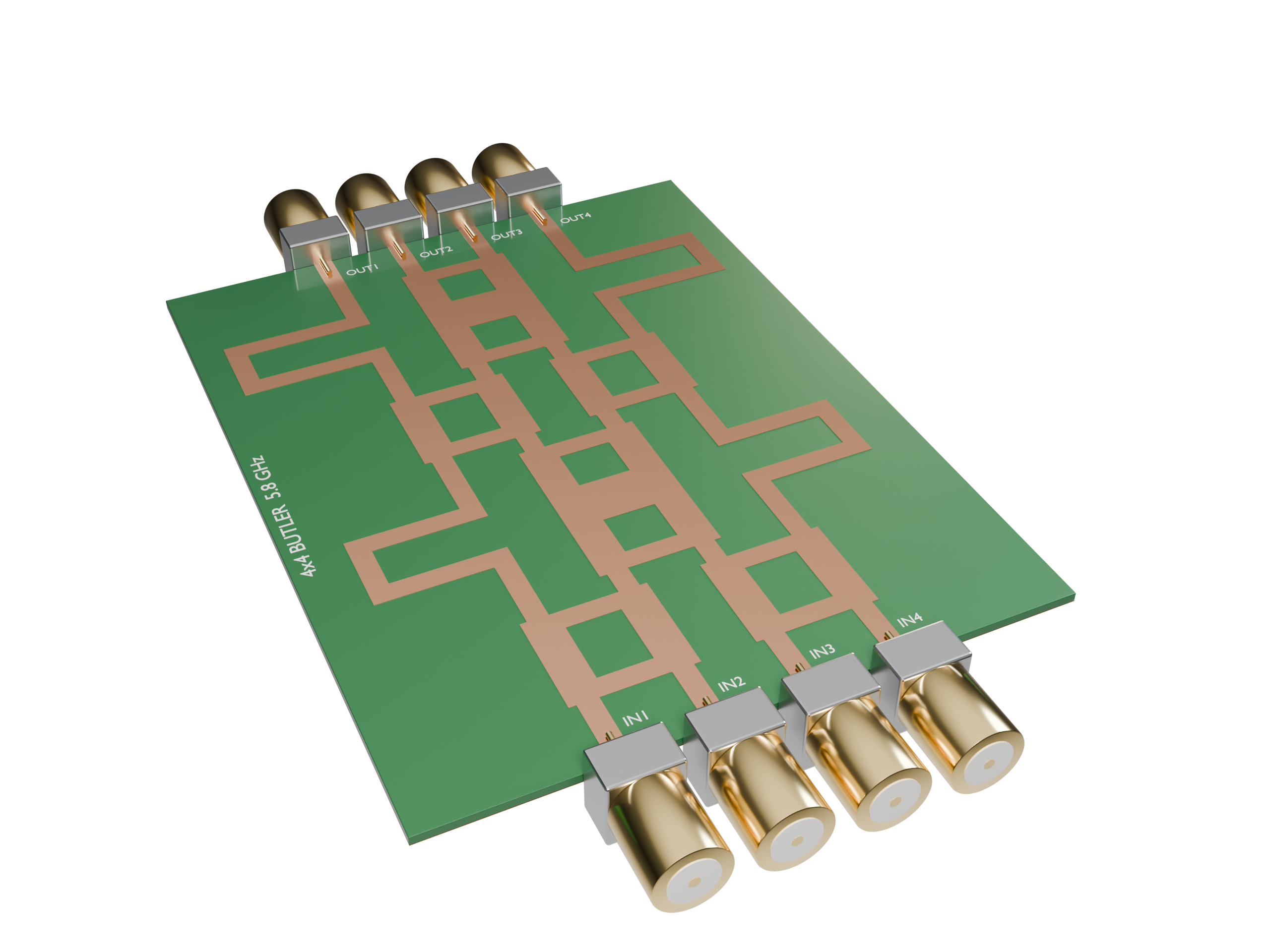
In this notebook we design, simulate and verify a complete 4×4 microstrip Butler matrix feeding a 1×4 patch array in the 5.8 GHz ISM band. The workflow is deliberately modular, which is how such networks are designed in practice:
- Design equations: synthesise 50 Ω, 35.4 Ω and 25 Ω microstrip lines on Rogers RO4003C.
- Layout-aware circuit model: an ideal transmission-line network generated from the same layout that we later simulate. It is used to size the phase-compensation lines in a fraction of a second.
- Full-wave verification of the building blocks with the TerminalComponentModeler: the 90° branch-line hybrid and the 0 dB crossover.
- Full-wave simulation of the complete 8-port Butler matrix and extraction of its amplitude/phase table.
- Beamforming: simulate a 1×4 inset-fed patch array, then combine its per-port radiation with the simulated Butler-matrix outputs to obtain the four switched beams, and compare with the array-factor prediction.
import os

import matplotlib.pyplot as plt
import numpy as np
import tidy3d as td
from scipy.optimize import brentq, minimize
from tidy3d import web

# The terminal component modeler is moving to the Flexcompute RF package.
# Try the new location first and fall back to the Tidy3D plugin.
try:
    from flexcompute.rf.tidy3d import (
        LumpedPort,
        TerminalComponentModeler,
        TerminalComponentModelerData,
    )
except ImportError:
    from tidy3d.plugins.smatrix import (
        LumpedPort,
        TerminalComponentModeler,
        TerminalComponentModelerData,
    )

td.config.logging.level = "ERROR"
os.makedirs("data", exist_ok=True)
os.makedirs("img", exist_ok=True)
Butler Matrix Theory
The 4×4 Butler matrix consists of four 90° (quadrature) hybrids, two 0 dB crossovers and two 45° phase shifters:
  in1 ─┐┌─ in2      in3 ─┐┌─ in4
     [Hybrid A]        [Hybrid B]
  │      └────╲ ╱────┘        │
 −45°          ╳  crossover  −45°
  │      ┌────╱ ╲────┐        │
     [Hybrid C]        [Hybrid D]
  │      └────╲ ╱────┘        │
  0°           ╳  crossover   0°
  │      ┌────╱ ╲────┐        │
 out1  out2        out3  out4
Each input splits into four outputs of equal amplitude ($|S|^2 = 1/4$, i.e. −6.02 dB), and the phase difference between neighbouring outputs is $\pm 45^\circ$ or $\pm 135^\circ$. With half-wavelength spacing ($k_0 d = \pi$) the four beams point at
| Progressive phase $\Delta\phi$ | $-135^\circ$ | $-45^\circ$ | $+45^\circ$ | $+135^\circ$ |
|---|---|---|---|---|
| Beam angle $\theta$ | $-48.6^\circ$ | $-14.5^\circ$ | $+14.5^\circ$ | $+48.6^\circ$ |
In a planar layout the lines that bypass the crossovers (lines 1 and 4) must have exactly the electrical length of the crossover's through path, plus a 45° offset in the first stage. Instead of computing those lengths by hand, we will let a circuit model of the actual layout choose them.
Substrate and Design Frequency
We use a 0.813 mm (32 mil) Rogers RO4003C laminate ($\varepsilon_r = 3.55$ design value, $\tan\delta = 0.0027$) with a solid ground plane. The metal layers are modelled as zero-thickness PEC sheets (td.PEC2D). Conductor loss could be included by replacing them with td.LossyMetalMedium.
Tidy3D uses micrometres as its length unit, so we define mm = 1e3.
mm = 1e3  # 1 mm in Tidy3D units (um)

f0 = 5.8e9  # design frequency (Hz)
f_min, f_max = 5.0e9, 6.6e9  # simulation band (Hz)
freqs = np.linspace(f_min, f_max, 81)  # includes f0 exactly
lambda0 = td.C_0 / f0  # free-space wavelength (um)

eps_r = 3.55  # RO4003C design Dk
tan_d = 0.0027  # RO4003C loss tangent
h_sub = 0.813 * mm  # substrate thickness

# conductivity reproducing tan(delta) at f0 (Tidy3D units: S/um)
sigma = 2 * np.pi * f0 * td.EPSILON_0 * eps_r * tan_d
substrate_medium = td.Medium(permittivity=eps_r, conductivity=sigma, name="RO4003C")
metal = td.PEC2D
air = td.Medium()

print(f"free-space wavelength at f0: {lambda0 / mm:.2f} mm")
free-space wavelength at f0: 51.69 mm
Microstrip Synthesis
The closed-form Hammerstad–Jensen equations give the characteristic impedance $Z_c$ and effective permittivity $\varepsilon_\mathrm{eff}$ of a microstrip line of width $W$. We invert them numerically to find the widths of the three line types we need:
- 50 Ω: port feeds, hybrid shunt arms, crossover outer arms and phase lines
- 35.4 Ω ($Z_0/\sqrt{2}$): hybrid and crossover series arms
- 25 Ω ($Z_0/2$): middle arm of the three-branch crossover
def eps_eff(W, h=h_sub, er=eps_r):
    """Hammerstad-Jensen effective permittivity of a microstrip line."""
    u = W / h
    a = (
        1
        + np.log((u**4 + (u / 52) ** 2) / (u**4 + 0.432)) / 49
        + np.log(1 + (u / 18.1) ** 3) / 18.7
    )
    b = 0.564 * ((er - 0.9) / (er + 3)) ** 0.053
    return (er + 1) / 2 + (er - 1) / 2 * (1 + 10 / u) ** (-a * b)


def z_char(W, h=h_sub):
    """Hammerstad-Jensen characteristic impedance (ohm) of a microstrip line."""
    u = W / h
    F = 6 + (2 * np.pi - 6) * np.exp(-((30.666 / u) ** 0.7528))
    return 60 / np.sqrt(eps_eff(W, h)) * np.log(F / u + np.sqrt(1 + (2 / u) ** 2))


def width_for(z0):
    """Line width (um) that gives a characteristic impedance z0."""
    return brentq(lambda w: z_char(w) - z0, 1.0, 20 * mm)


def quarter_wave(W, f=f0):
    """Quarter guided wavelength (um) of a line of width W."""
    return td.C_0 / f / np.sqrt(eps_eff(W)) / 4


W50, W35, W25 = width_for(50.0), width_for(50.0 / np.sqrt(2)), width_for(25.0)
q50, q35, q25 = quarter_wave(W50), quarter_wave(W35), quarter_wave(W25)

print(f"{'Z0 (ohm)':>9} {'W (mm)':>8} {'eps_eff':>8} {'lambda_g/4 (mm)':>16}")
for z, W, q in [(50, W50, q50), (35.36, W35, q35), (25, W25, q25)]:
    print(f"{z:9.2f} {W / mm:8.3f} {eps_eff(W):8.3f} {q / mm:16.3f}")
 Z0 (ohm)   W (mm)  eps_eff  lambda_g/4 (mm)
    50.00    1.821    2.787            7.741
    35.36    3.052    2.909            7.576
    25.00    4.841    3.025            7.430
Layout Generator and Layout-Aware Circuit Model
Every circuit in this notebook is described as a list of microstrip centre-line segments (node_a, node_b, width) on a Manhattan grid. One generator therefore serves two purposes:
- Circuit model: each segment becomes an ideal transmission line with $Z_c(W)$ and $\varepsilon_\mathrm{eff}(W)$. Its two-port admittance matrix $$Y = \frac{1}{Z_c}\begin{pmatrix} \coth\gamma\ell & -\operatorname{csch}\gamma\ell \\ -\operatorname{csch}\gamma\ell & \coth\gamma\ell \end{pmatrix}$$ is stamped into a nodal admittance matrix. The internal nodes are then eliminated (Kron reduction) and the result is converted to an S-matrix referenced to 50 Ω. Junction parasitics are ignored, so this model is only accurate to first order, but it is instantaneous.
- Full-wave model: each segment becomes a PEC rectangle, and every node gets a junction pad sized by the widths that meet there.
The circuit model uses the engineering $e^{+j\omega t}$ convention, while Tidy3D uses $e^{-i\omega t}$. We therefore complex-conjugate the circuit S-parameters whenever we compare them with the simulations.
All lines run along the $y$ direction from the inputs (bottom) to the outputs (top). The four signal lines sit at a pitch of $p = \lambda_{g,50}/4$, so the hybrids and crossovers fit exactly between neighbouring lines.
class Layout:
    """Manhattan microstrip layout made of centre-line segments."""

    def __init__(self):
        self.segments = []  # (node_a, node_b, width) with nodes as integer nm tuples
        self.ports = {}  # name -> node
        self.extra_points = []  # (x, y) points the board must also cover, e.g. patch corners

    @staticmethod
    def node(x, y):
        return (round(x * 1e3), round(y * 1e3))  # um -> integer nm key

    def line(self, x0, y0, x1, y1, W):
        assert x0 == x1 or y0 == y1, "only Manhattan segments are supported"
        self.segments.append((self.node(x0, y0), self.node(x1, y1), W))

    def port(self, name, x, y):
        self.ports[name] = self.node(x, y)

    # ---------- building blocks ----------
    def hybrid(self, xl, xr, y):
        """90-degree branch-line hybrid between x=xl and x=xr, starting at height y."""
        self.line(xl, y, xl, y + q35, W35)  # series arms (signal flows along +y)
        self.line(xr, y, xr, y + q35, W35)
        self.line(xl, y, xr, y, W50)  # shunt arms
        self.line(xl, y + q35, xr, y + q35, W50)
        return y + q35

    def crossover(self, xl, xr, y):
        """0 dB three-branch crossover (two cascaded hybrids)."""
        for x in (xl, xr):
            self.line(x, y, x, y + q35, W35)
            self.line(x, y + q35, x, y + 2 * q35, W35)
        self.line(xl, y, xr, y, W50)
        self.line(xl, y + q35, xr, y + q35, W25)
        self.line(xl, y + 2 * q35, xr, y + 2 * q35, W50)
        return y + 2 * q35

    def phase_line(self, x, y, length, detour, side, gap=6 * mm):
        """Straight 50-ohm line of height `length` with a rectangular detour of depth `detour`.

        The detour adds 2*detour of path length; side=-1 bulges towards -x, +1 towards +x.
        """
        ya, yb, xo = (
            y + length / 2 - gap / 2,
            y + length / 2 + gap / 2,
            x + side * detour,
        )
        self.line(x, y, x, ya, W50)
        self.line(x, ya, xo, ya, W50)
        self.line(xo, ya, xo, yb, W50)
        self.line(xo, yb, x, yb, W50)
        self.line(x, yb, x, y + length, W50)
        return y + length

    # ---------- geometry helpers ----------
    def bounds(self):
        pts = np.array([n for s in self.segments for n in s[:2]]) * 1e-3
        pad = max(s[2] for s in self.segments) / 2
        lo, hi = pts.min(axis=0) - pad, pts.max(axis=0) + pad
        if self.extra_points:
            ep = np.array(self.extra_points)
            lo, hi = np.minimum(lo, ep.min(axis=0)), np.maximum(hi, ep.max(axis=0))
        return lo, hi

    def rectangles(self):
        """Return metal rectangles (xmin, ymin, xmax, ymax) for segments and junction pads."""
        rects, pads = [], {}
        for a, b, W in self.segments:
            (xa, ya), (xb, yb) = np.array(a) * 1e-3, np.array(b) * 1e-3
            if ya == yb:  # horizontal
                rects.append((min(xa, xb), ya - W / 2, max(xa, xb), ya + W / 2))
            else:  # vertical
                rects.append((xa - W / 2, min(ya, yb), xa + W / 2, max(ya, yb)))
            for n in (a, b):
                wx, wy = pads.get(n, (0.0, 0.0))
                # vertical lines set the pad width in x, horizontal lines the pad height in y
                pads[n] = (max(wx, W), wy) if ya != yb else (wx, max(wy, W))
        for n, (wx, wy) in pads.items():
            wx, wy = wx or wy, wy or wx
            x, y = np.array(n) * 1e-3
            rects.append((x - wx / 2, y - wy / 2, x + wx / 2, y + wy / 2))
        return rects

    def plot(self, ax=None, **kw):
        ax = ax or plt.gca()
        for x0, y0, x1, y1 in self.rectangles():
            ax.add_patch(
                plt.Rectangle(
                    (x0 / mm, y0 / mm),
                    (x1 - x0) / mm,
                    (y1 - y0) / mm,
                    color="#b87333",
                    lw=0,
                )
            )
        for name, n in self.ports.items():
            x, y = np.array(n) * 1e-6
            ax.annotate(
                name,
                (x, y),
                ha="center",
                va="center",
                fontsize=8,
                color="k",
                bbox={"boxstyle": "round", "fc": "w", "alpha": 0.8},
            )
        ax.set_aspect("equal")
        ax.autoscale()
        ax.set_xlabel("x (mm)")
        ax.set_ylabel("y (mm)")
        return ax


def circuit_smatrix(layout, f, z_ref=50.0):
    """Ideal transmission-line S-matrix of a layout (engineering e^{+jwt} convention)."""
    nodes = sorted({n for s in layout.segments for n in s[:2]})
    idx = {n: i for i, n in enumerate(nodes)}
    Y = np.zeros((len(nodes), len(nodes)), dtype=complex)
    for a, b, W in layout.segments:
        length = np.hypot(a[0] - b[0], a[1] - b[1]) * 1e-3  # um
        gl = 2j * np.pi * f * np.sqrt(eps_eff(W)) / td.C_0 * length
        zc = z_char(W)
        y11, y12 = 1 / (zc * np.tanh(gl)), -1 / (zc * np.sinh(gl))
        i, j = idx[a], idx[b]
        Y[i, i] += y11
        Y[j, j] += y11
        Y[i, j] += y12
        Y[j, i] += y12
    names = list(layout.ports)
    P = [idx[layout.ports[k]] for k in names]
    I = [i for i in range(len(nodes)) if i not in P]
    Yp = Y[np.ix_(P, P)] - Y[np.ix_(P, I)] @ np.linalg.solve(
        Y[np.ix_(I, I)], Y[np.ix_(I, P)]
    )
    E = np.eye(len(P)) / z_ref
    return names, (E - Yp) @ np.linalg.inv(E + Yp)
Building Blocks
We now create stand-alone layouts of the branch-line hybrid and the crossover, each with 50 Ω feed lines of length L_feed on all four corners. These are exactly the layouts we will simulate later.
L_feed = 6 * mm  # feed-line length in front of every port
pitch = q50  # spacing between neighbouring signal lines


def make_hybrid():
    lay = Layout()
    xl, xr = -pitch / 2, pitch / 2
    for x, n in [(xl, "1"), (xr, "2")]:
        lay.line(x, 0, x, L_feed, W50)
        lay.port(n, x, 0)
    y = lay.hybrid(xl, xr, L_feed)
    for x, n in [(xl, "3"), (xr, "4")]:
        lay.line(x, y, x, y + L_feed, W50)
        lay.port(n, x, y + L_feed)
    return lay


def make_crossover():
    lay = Layout()
    xl, xr = -pitch / 2, pitch / 2
    for x, n in [(xl, "1"), (xr, "2")]:
        lay.line(x, 0, x, L_feed, W50)
        lay.port(n, x, 0)
    y = lay.crossover(xl, xr, L_feed)
    for x, n in [(xl, "3"), (xr, "4")]:
        lay.line(x, y, x, y + L_feed, W50)
        lay.port(n, x, y + L_feed)
    return lay


hybrid_layout, crossover_layout = make_hybrid(), make_crossover()


def print_column(layout, src="1"):
    names, S = circuit_smatrix(layout, f0)
    S = S.conj()  # Tidy3D phase convention
    j = names.index(src)
    for i, n in enumerate(names):
        print(
            f"  S{n}{src}: {20 * np.log10(abs(S[i, j]) + 1e-15):8.2f} dB  {np.angle(S[i, j], deg=True):8.1f} deg"
        )


print("Branch-line hybrid (circuit model, f0):")
print_column(hybrid_layout)
print("Crossover (circuit model, f0):")
print_column(crossover_layout)

fig, ax = plt.subplots(1, 2, figsize=(8, 5))
hybrid_layout.plot(ax[0]).set_title("branch-line hybrid")
crossover_layout.plot(ax[1]).set_title("0 dB crossover")
plt.tight_layout()
plt.show()
Branch-line hybrid (circuit model, f0):
  S11:  -143.00 dB      49.5 deg
  S21:  -143.00 dB     -40.5 deg
  S31:    -3.01 dB    -130.5 deg
  S41:    -3.01 dB     -40.5 deg
Crossover (circuit model, f0):
  S11:   -53.34 dB     147.0 deg
  S21:   -23.65 dB     143.3 deg
  S31:   -53.34 dB     147.1 deg
  S41:    -0.02 dB      53.3 deg
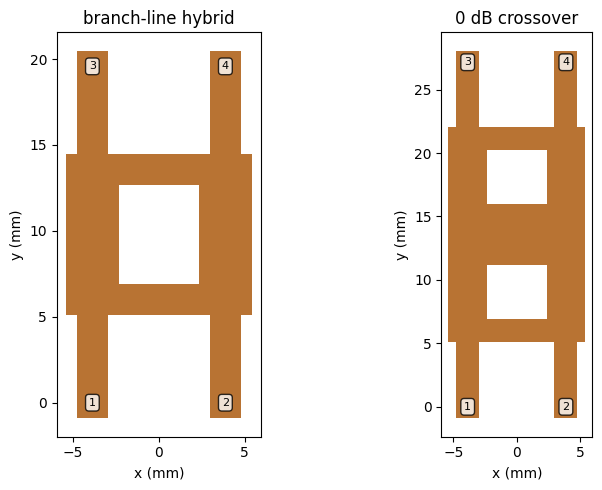
The ideal hybrid splits the power equally between ports 3 and 4 (−3.01 dB) with a 90° phase difference, and ports 1 and 2 are perfectly matched and isolated. The crossover sends all the power from port 1 to the diagonally opposite port 4.
Complete Butler Matrix
The full matrix stacks the blocks along $y$: hybrids A/B → crossover + phase lines → hybrids C/D → crossover + reference lines. Short 50 Ω connecting lines of length L_conn separate the stages. The bypass lines 1 and 4 bulge outwards, by detour1 in the first stage and detour2 in the second.
L_conn = 4 * mm  # connecting lines between stages
X_lines = [(k - 1.5) * pitch for k in range(4)]  # x position of signal lines 1..4


def make_butler(detour1, detour2):
    lay = Layout()
    for k, x in enumerate(X_lines):
        lay.line(x, 0, x, L_feed, W50)
        lay.port(f"in{k + 1}", x, 0)

    def connect(y):
        for x in X_lines:
            lay.line(x, y, x, y + L_conn, W50)
        return y + L_conn

    y = L_feed
    lay.hybrid(X_lines[0], X_lines[1], y)  # hybrid A
    y = lay.hybrid(X_lines[2], X_lines[3], y)  # hybrid B
    y = connect(y)
    lay.phase_line(X_lines[0], y, 2 * q35, detour1, side=-1)  # 45-degree phase lines
    lay.phase_line(X_lines[3], y, 2 * q35, detour1, side=+1)
    y = lay.crossover(X_lines[1], X_lines[2], y)
    y = connect(y)
    lay.hybrid(X_lines[0], X_lines[1], y)  # hybrid C
    y = lay.hybrid(X_lines[2], X_lines[3], y)  # hybrid D
    y = connect(y)
    lay.phase_line(X_lines[0], y, 2 * q35, detour2, side=-1)  # 0-degree reference lines
    lay.phase_line(X_lines[3], y, 2 * q35, detour2, side=+1)
    y = lay.crossover(X_lines[1], X_lines[2], y)
    for k, x in enumerate(X_lines):
        lay.line(x, y, x, y + L_feed, W50)
        lay.port(f"out{k + 1}", x, y + L_feed)
    return lay


IN = [f"in{k}" for k in range(1, 5)]
OUT = [f"out{k}" for k in range(1, 5)]


def butler_table(S, names):
    """Return |S_out,in| (4x4) and progressive phases (4x3, deg) for each input."""
    T = np.array([[S[names.index(o), names.index(i)] for i in IN] for o in OUT])
    dphi = np.angle(T[1:, :] / T[:-1, :], deg=True)
    return T, dphi


def phase_error(params):
    names, S = circuit_smatrix(make_butler(*(np.array(params) * mm)), f0)
    T, _ = butler_table(S, names)
    z = T[1:, :] / T[:-1, :]
    z /= abs(z)
    return np.sum(
        abs(z - z.mean(axis=0)) ** 2
    )  # zero for a perfectly uniform phase progression


# coarse grid search followed by a local refinement
grid = np.arange(1.0, 30.0, 0.5)
err = np.array([[phase_error((a, b)) for b in grid] for a in grid])
i, j = np.unravel_index(err.argmin(), err.shape)
res = minimize(
    phase_error, [grid[i], grid[j]], method="Nelder-Mead", options={"xatol": 1e-3}
)
detour1, detour2 = res.x * mm
print(f"detour1 = {detour1 / mm:.3f} mm, detour2 = {detour2 / mm:.3f} mm")

butler_layout = make_butler(detour1, detour2)
names_c, S_c = circuit_smatrix(butler_layout, f0)
T_c, dphi_c = butler_table(S_c.conj(), names_c)  # conj -> Tidy3D phase convention
for k, i_name in enumerate(IN):
    print(
        f"{i_name}: |S| = {np.round(20 * np.log10(abs(T_c[:, k])), 2)} dB, "
        f"progressive phase = {np.round(dphi_c[:, k], 1)} deg"
    )

fig, ax = plt.subplots(figsize=(6, 7))
butler_layout.plot(ax).set_title("4x4 Butler matrix layout")
plt.savefig("img/butler_matrix_layout.png", dpi=120, bbox_inches="tight")
plt.show()
detour1 = 10.003 mm, detour2 = 11.939 mm
in1: |S| = [-6.05 -6.05 -5.99 -6.02] dB, progressive phase = [134.8 134.9 135.2] deg
in2: |S| = [-6.03 -6.03 -6.05 -6.02] dB, progressive phase = [-44.8 -44.9 -45.2] deg
in3: |S| = [-6.02 -6.05 -6.03 -6.03] dB, progressive phase = [45.2 44.9 44.8] deg
in4: |S| = [-6.02 -5.99 -6.05 -6.05] dB, progressive phase = [-135.2 -134.9 -134.8] deg
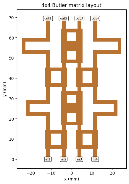
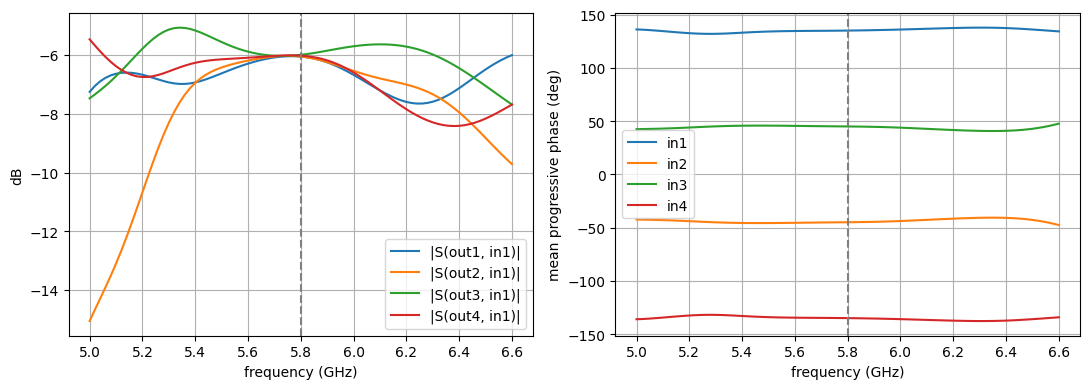
The circuit model confirms the textbook behaviour: every input divides equally into the four outputs (≈ −6.02 dB), and the four inputs produce progressive phases of about ±45° and ±135°. The bandwidth of the ideal network is shown below. The output amplitude and phase stay well balanced across the 5.6–6.0 GHz range.
tables = [
    butler_table(circuit_smatrix(butler_layout, f)[1].conj(), names_c) for f in freqs
]
mags = np.array([20 * np.log10(abs(T)) for T, _ in tables])  # (f, out, in)
phs = np.array([dphi for _, dphi in tables])  # (f, 3, in)

fig, ax = plt.subplots(1, 2, figsize=(11, 4))
for o in range(4):
    ax[0].plot(freqs / 1e9, mags[:, o, 0], label=f"|S(out{o + 1}, in1)|")
for k in range(4):
    ax[1].plot(freqs / 1e9, phs[:, :, k].mean(axis=1), label=f"in{k + 1}")
ax[0].set_ylabel("dB")
ax[1].set_ylabel("mean progressive phase (deg)")
for a in ax:
    a.set_xlabel("frequency (GHz)")
    a.axvline(f0 / 1e9, color="gray", ls="--")
    a.legend()
    a.grid(True)
plt.tight_layout()
plt.show()
Full-Wave Models
The helper below turns any Layout into a td.Simulation with:
- the RO4003C substrate and a PEC ground plane. For the circuits they extend through the PML, so surface waves are absorbed and no artificial board edges are introduced. For the antennas we use a finite board, which is cut at the port planes and extends 3 mm beyond the metal elsewhere,
- the metal rectangles as
td.PEC2Dsheets on top of the substrate, - an automatic non-uniform grid with a LayerRefinementSpec that resolves the substrate thickness and refines the metal corners, plus a mesh override that resolves the line widths,
- PML on all sides, $\lambda_0/4$ (circuits) or $\lambda_0/2$ (antennas) away from the board.
Each port is a 50 Ω LumpedPort that spans the substrate between the ground plane and the end of a feed line.
def make_simulation(
    layout,
    extra_structures=(),
    monitors=(),
    pad_xy=None,
    pad_top=None,
    pad_bottom=None,
    run_time=20e-9,
    dl_xy=0.4 * mm,
    infinite_board=True,
):
    pad_xy = lambda0 / 4 if pad_xy is None else pad_xy
    pad_top = lambda0 / 4 if pad_top is None else pad_top
    pad_bottom = lambda0 / 8 if pad_bottom is None else pad_bottom
    (xmin, ymin), (xmax, ymax) = layout.bounds()
    port_y = [np.array(n)[1] * 1e-3 for n in layout.ports.values()]
    margin = 3 * mm
    # the board ends at the port planes (ports sit at the board edge); elsewhere it has a margin
    y_lo = ymin if np.isclose(min(port_y), ymin, atol=W50) else ymin - margin
    y_hi = ymax if np.isclose(max(port_y), ymax, atol=W50) else ymax + margin
    y_lo, y_hi = min(y_lo, min(port_y)), max(y_hi, max(port_y))
    sub_min = np.array([xmin - margin, y_lo, 0])
    sub_max = np.array([xmax + margin, y_hi, h_sub])
    if infinite_board:
        # circuits: substrate and ground run through the PML, which absorbs surface waves cleanly
        board_min, board_max = (-td.inf, -td.inf, 0), (td.inf, td.inf, h_sub)
    else:
        # antennas: finite board so that edge diffraction and the back lobe are captured
        board_min, board_max = sub_min, sub_max
    substrate = td.Structure(
        geometry=td.Box.from_bounds(board_min, board_max), medium=substrate_medium
    )
    ground = td.Structure(
        geometry=td.Box.from_bounds(
            (board_min[0], board_min[1], 0), (board_max[0], board_max[1], 0)
        ),
        medium=metal,
    )
    traces = [
        td.Structure(
            geometry=td.Box.from_bounds((x0, y0, h_sub), (x1, y1, h_sub)), medium=metal
        )
        for (x0, y0, x1, y1) in layout.rectangles()
    ]

    sim_min = sub_min - np.array([pad_xy, pad_xy, pad_bottom])
    sim_max = sub_max + np.array([pad_xy, pad_xy, pad_top])
    center, size = (sim_min + sim_max) / 2, sim_max - sim_min

    metal_refinement = td.LayerRefinementSpec(
        center=(center[0], center[1], h_sub),
        size=(td.inf, td.inf, 0),
        axis=2,
        min_steps_along_axis=1,
        corner_refinement=td.GridRefinement(dl=dl_xy / 4, num_cells=2),
    )
    substrate_refinement = td.LayerRefinementSpec(
        center=(center[0], center[1], h_sub / 2),
        size=(td.inf, td.inf, h_sub),
        axis=2,
        min_steps_along_axis=4,
        corner_refinement=None,
    )
    trace_override = td.MeshOverrideStructure(
        geometry=td.Box.from_bounds(sub_min, sub_max), dl=(dl_xy, dl_xy, None)
    )

    return td.Simulation(
        center=tuple(center),
        size=tuple(size),
        structures=[substrate, ground, *traces, *extra_structures],
        monitors=list(monitors),
        grid_spec=td.GridSpec.auto(
            min_steps_per_wvl=20,
            wavelength=td.C_0 / f_max,
            layer_refinement_specs=[substrate_refinement, metal_refinement],
            override_structures=[trace_override],
        ),
        boundary_spec=td.BoundarySpec.all_sides(td.PML()),
        run_time=run_time,
        plot_length_units="mm",
    )


def make_ports(layout, names=None):
    names = names or list(layout.ports)
    return [
        LumpedPort(
            center=(
                np.array(layout.ports[n])[0] * 1e-3,
                np.array(layout.ports[n])[1] * 1e-3,
                h_sub / 2,
            ),
            size=(W50, 0, h_sub),
            voltage_axis=2,
            impedance=50,
            name=n,
        )
        for n in names
    ]


def run_modeler(modeler, task_name):
    """Run a component modeler, re-using results that are already on disk."""
    path = f"data/{task_name}.hdf5"
    if (
        os.path.exists(path)
        and TerminalComponentModelerData.from_file(path).modeler == modeler
    ):
        return TerminalComponentModelerData.from_file(path)
    job = web.Job(simulation=modeler, task_name=task_name, verbose=True)
    print(f"{task_name}: estimated cost = {job.estimate_cost():.3f} FlexCredits")
    return job.run(path=path)


def sparams(modeler_data):
    """S-matrix as an xarray DataArray with dims (f, port_out, port_in)."""
    return modeler_data.smatrix().data
Step 1: Branch-Line Hybrid
The hybrid is symmetric, so one excitation (port 1) gives the complete scattering behaviour. We use run_only to launch just that simulation.
hybrid_sim = make_simulation(hybrid_layout)
hybrid_modeler = TerminalComponentModeler(
    simulation=hybrid_sim,
    ports=make_ports(hybrid_layout),
    freqs=freqs,
    run_only=("1",),
)

fig, ax = plt.subplots(1, 2, figsize=(11, 5))
hybrid_modeler.plot_sim(z=h_sub, ax=ax[0])
hybrid_sim.plot_grid(z=h_sub, ax=ax[0], linewidth=0.2)
hybrid_modeler.plot_sim(x=-pitch / 2, ax=ax[1])
ax[1].set_aspect("auto")
plt.tight_layout()
plt.show()
print(f"grid cells: {hybrid_sim.num_cells / 1e6:.2f} M")
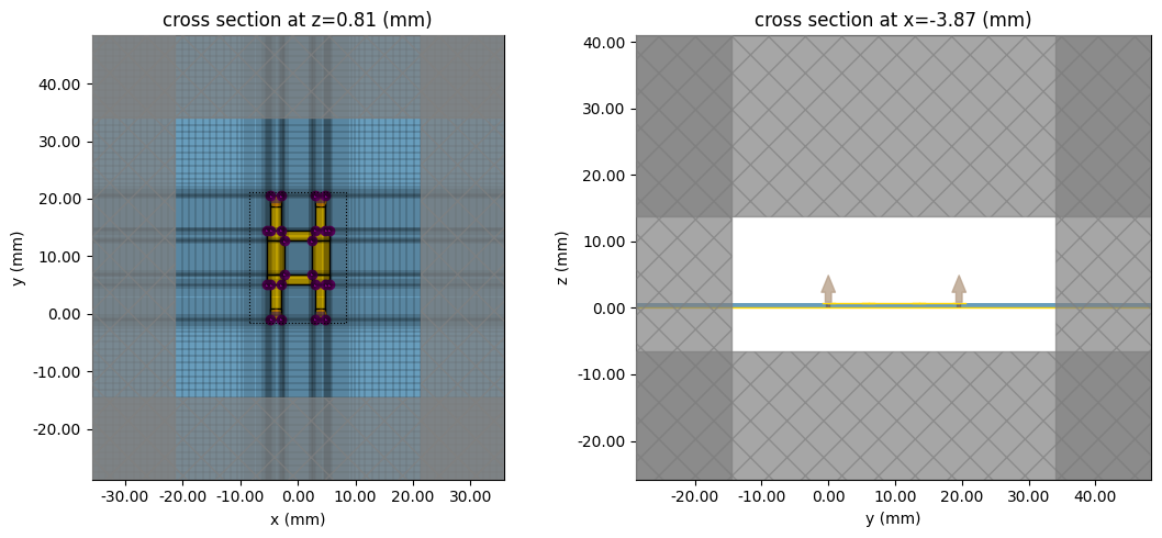
grid cells: 0.99 M
hybrid_data = run_modeler(hybrid_modeler, "butler_hybrid")
S_h = sparams(hybrid_data)
def compare_plot(S_fdtd, layout, src, title):
    names, _ = circuit_smatrix(layout, f0)
    S_circ = np.array([circuit_smatrix(layout, f)[1].conj() for f in freqs])
    j = names.index(src)
    fig, ax = plt.subplots(1, 2, figsize=(11, 4))
    for i, n in enumerate(names):
        s = S_fdtd.sel(port_in=src, port_out=n)
        (l,) = ax[0].plot(freqs / 1e9, 20 * np.log10(abs(s)), label=f"S{n}{src}")
        ax[0].plot(
            freqs / 1e9,
            20 * np.log10(abs(S_circ[:, i, j]) + 1e-6),
            "--",
            color=l.get_color(),
        )
    ax[0].set_ylim(-40, 1)
    ax[0].set_ylabel("|S| (dB)")
    ax[0].set_title(f"{title}: FDTD (solid) vs circuit (dashed)")
    return fig, ax, names, S_circ


fig, ax, names_h, S_hc = compare_plot(S_h, hybrid_layout, "1", "hybrid")
dphi_fdtd = np.angle(
    S_h.sel(port_in="1", port_out="3") / S_h.sel(port_in="1", port_out="4"), deg=True
)
dphi_circ = np.angle(
    S_hc[:, names_h.index("3"), 0] / S_hc[:, names_h.index("4"), 0], deg=True
)
ax[1].plot(freqs / 1e9, dphi_fdtd, label="FDTD")
ax[1].plot(freqs / 1e9, dphi_circ, "--", label="circuit")
ax[1].set_ylabel("phase(S31) - phase(S41) (deg)")
for a in ax:
    a.set_xlabel("frequency (GHz)")
    a.axvline(f0 / 1e9, color="gray", ls=":")
    a.grid(True)
    a.legend()
plt.tight_layout()
plt.show()
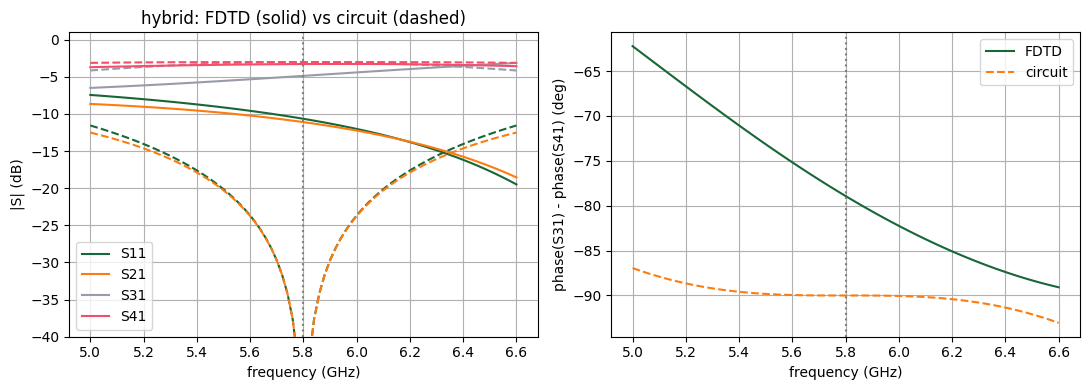
The full-wave hybrid closely follows the circuit model. Any small downward shift of the centre frequency comes from the T-junction parasitics, which the ideal line model neglects. If you need a better centre frequency, shorten q35 and pitch by a few percent and rerun this cell. The building block is cheap, so tuning it here first is much faster than tuning the full matrix.
Step 2: 0 dB Crossover
crossover_sim = make_simulation(crossover_layout)
crossover_modeler = TerminalComponentModeler(
    simulation=crossover_sim,
    ports=make_ports(crossover_layout),
    freqs=freqs,
    run_only=("1",),
)
crossover_modeler.plot_sim(z=h_sub)
plt.show()
print(f"grid cells: {crossover_sim.num_cells / 1e6:.2f} M")
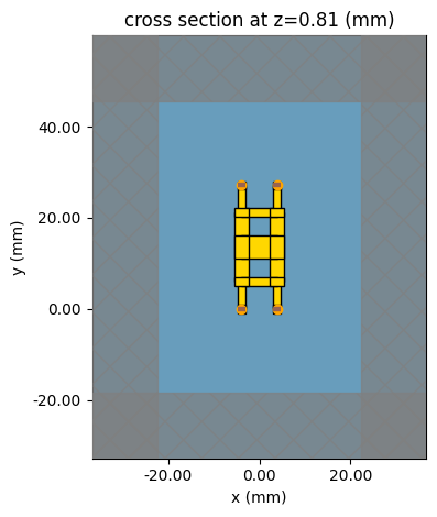
grid cells: 1.35 M
crossover_data = run_modeler(crossover_modeler, "butler_crossover")
S_x = sparams(crossover_data)

fig, ax, names_x, S_xc = compare_plot(S_x, crossover_layout, "1", "crossover")
ax[1].plot(
    freqs / 1e9, np.angle(S_x.sel(port_in="1", port_out="4"), deg=True), label="FDTD"
)
ax[1].plot(
    freqs / 1e9,
    np.angle(S_xc[:, names_x.index("4"), 0], deg=True),
    "--",
    label="circuit",
)
ax[1].set_ylabel("phase(S41) (deg)")
for a in ax:
    a.set_xlabel("frequency (GHz)")
    a.axvline(f0 / 1e9, color="gray", ls=":")
    a.grid(True)
    a.legend()
plt.tight_layout()
plt.show()
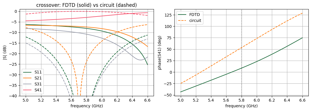
Step 3: Complete 4×4 Butler Matrix
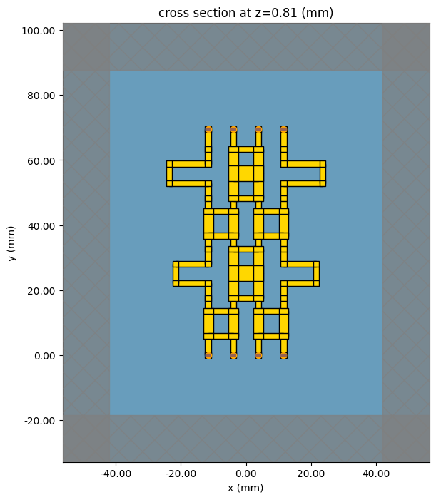
We now simulate the whole 8-port network. Only the four inputs need to be excited, because the four S-matrix columns S(:, in_i) contain everything we need for beamforming. run_only=IN therefore halves the cost compared with a full 8×8 characterisation.
butler_sim = make_simulation(butler_layout, run_time=30e-9)
butler_modeler = TerminalComponentModeler(
    simulation=butler_sim,
    ports=make_ports(butler_layout),
    freqs=freqs,
    run_only=tuple(IN),
)
fig, ax = plt.subplots(figsize=(7, 8))
butler_modeler.plot_sim(z=h_sub, ax=ax)
plt.show()
print(f"grid cells: {butler_sim.num_cells / 1e6:.2f} M")
grid cells: 6.93 M
butler_data = run_modeler(butler_modeler, "butler_matrix_4x4")
S_b = sparams(butler_data)
Amplitude and Phase Table at 5.8 GHz
T_fdtd = np.array(
    [
        [
            complex(S_b.sel(f=f0, method="nearest").sel(port_out=o, port_in=i))
            for i in IN
        ]
        for o in OUT
    ]
)
dphi_fdtd = np.angle(T_fdtd[1:, :] / T_fdtd[:-1, :], deg=True)

print(f"{'':6}" + "".join(f"{i:>12}" for i in IN))
for r, o in enumerate(OUT):
    print(
        f"{o:6}"
        + "".join(f"{20 * np.log10(abs(T_fdtd[r, c])):9.2f} dB" for c in range(4))
    )
print("\nprogressive phase (deg)   FDTD          circuit")
for c, i in enumerate(IN):
    print(f"  {i}: {np.round(dphi_fdtd[:, c], 1)}   {np.round(dphi_c[:, c], 1)}")
print(
    "\ninput reflection |S_ii| at f0 (dB):",
    [
        round(
            float(
                20
                * np.log10(
                    abs(S_b.sel(f=f0, method="nearest").sel(port_out=i, port_in=i))
                )
            ),
            1,
        )
        for i in IN
    ],
)
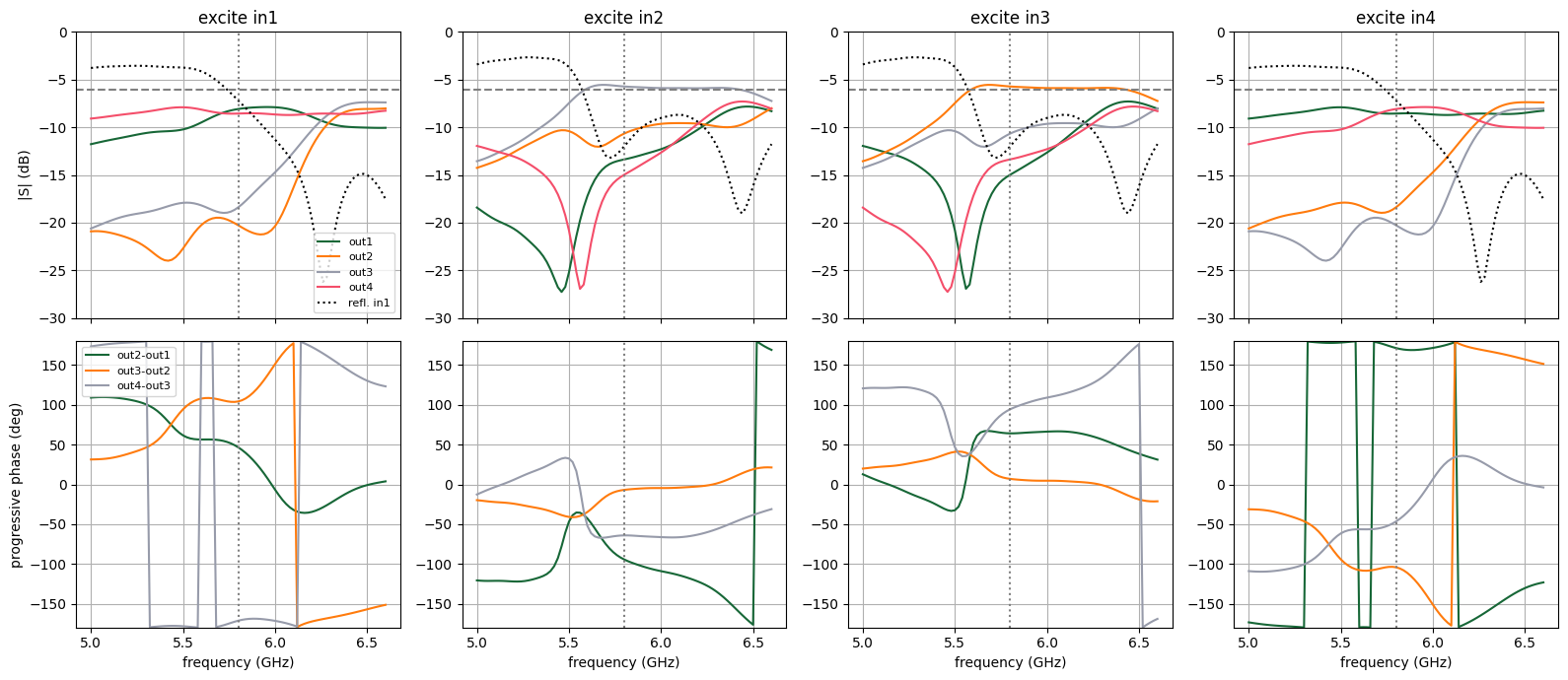
               in1         in2         in3         in4
out1      -8.08 dB   -13.37 dB   -14.98 dB    -8.56 dB
out2     -20.27 dB   -10.66 dB    -5.72 dB   -18.38 dB
out3     -18.39 dB    -5.72 dB   -10.66 dB   -20.28 dB
out4      -8.56 dB   -14.98 dB   -13.37 dB    -8.08 dB

progressive phase (deg)   FDTD          circuit
  in1: [  46.6  104.3 -171.4]   [134.8 134.9 135.2]
  in2: [-94.5  -6.9 -64.2]   [-44.8 -44.9 -45.2]
  in3: [64.2  6.9 94.5]   [45.2 44.9 44.8]
  in4: [ 171.4 -104.3  -46.6]   [-135.2 -134.9 -134.8]

input reflection |S_ii| at f0 (dB): [-7.2, -12.0, -12.0, -7.2]
fig, ax = plt.subplots(2, 4, figsize=(16, 7), sharex=True)
for c, i in enumerate(IN):
    for o in OUT:
        ax[0, c].plot(
            freqs / 1e9, 20 * np.log10(abs(S_b.sel(port_in=i, port_out=o))), label=o
        )
    ax[0, c].plot(
        freqs / 1e9,
        20 * np.log10(abs(S_b.sel(port_in=i, port_out=i))),
        "k:",
        label=f"refl. {i}",
    )
    ax[0, c].axhline(-6.02, color="gray", ls="--")
    ax[0, c].set_ylim(-30, 0)
    ax[0, c].set_title(f"excite {i}")
    s = np.array([S_b.sel(port_in=i, port_out=o).values for o in OUT])
    for k in range(3):
        ax[1, c].plot(
            freqs / 1e9,
            np.angle(s[k + 1] / s[k], deg=True),
            label=f"out{k + 2}-out{k + 1}",
        )
    ax[1, c].set_ylim(-180, 180)
    ax[1, c].set_xlabel("frequency (GHz)")
for a in ax.ravel():
    a.axvline(f0 / 1e9, color="gray", ls=":")
    a.grid(True)
ax[0, 0].set_ylabel("|S| (dB)")
ax[1, 0].set_ylabel("progressive phase (deg)")
ax[0, 0].legend(fontsize=8)
ax[1, 0].legend(fontsize=8)
plt.tight_layout()
plt.show()
Step 4: 1×4 Inset-Fed Patch Array
The array elements are rectangular patches on the same substrate, spaced by $d = \lambda_0/2$ along $x$, so the beams scan in the $xz$ plane. The patch dimensions come from the transmission-line model. An inset feed of depth $y_0$ matches the edge resistance to 50 Ω:
$$W = \frac{c}{2f_0}\sqrt{\frac{2}{\varepsilon_r+1}},\qquad L = \frac{c}{2f_0\sqrt{\varepsilon_\mathrm{eff}}} - 2\Delta L,\qquad R_\mathrm{in}(y_0) = R_\mathrm{edge}\cos^2\!\left(\frac{\pi y_0}{L}\right).$$
from scipy.integrate import quad
from scipy.special import j0

W_patch = td.C_0 / (2 * f0) * np.sqrt(2 / (eps_r + 1))
ee_p = (eps_r + 1) / 2 + (eps_r - 1) / 2 / np.sqrt(1 + 12 * h_sub / W_patch)
dL = (
    0.412
    * h_sub
    * (ee_p + 0.3)
    * (W_patch / h_sub + 0.264)
    / ((ee_p - 0.258) * (W_patch / h_sub + 0.8))
)
L_patch = td.C_0 / (2 * f0 * np.sqrt(ee_p)) - 2 * dL

k0 = 2 * np.pi / lambda0
G1 = W_patch / (120 * lambda0) * (1 - (k0 * h_sub) ** 2 / 24)
G12 = quad(
    lambda t: (
        (np.sin(k0 * W_patch / 2 * np.cos(t)) / np.cos(t)) ** 2
        * np.sin(t) ** 3
        * j0(k0 * L_patch * np.sin(t))
    ),
    0,
    np.pi,
)[0] / (120 * np.pi**2)
R_edge = 1 / (2 * (G1 + G12))
y0_inset = L_patch / np.pi * np.arccos(np.sqrt(50 / R_edge))
gap_inset = 1.0 * mm  # notch gap on each side of the feed
L_feed_patch = 10 * mm
d_elem = lambda0 / 2

print(
    f"W = {W_patch / mm:.2f} mm, L = {L_patch / mm:.2f} mm, R_edge = {R_edge:.0f} ohm, "
    f"inset y0 = {y0_inset / mm:.2f} mm, spacing d = {d_elem / mm:.2f} mm"
)
W = 17.13 mm, L = 13.47 mm, R_edge = 149 ohm, inset y0 = 4.08 mm, spacing d = 25.84 mm
def make_patch_array(n_elem=4, L_p=L_patch):
    """Feed lines as a Layout (for ports/substrate) plus patch structures (inset patch = 3 boxes)."""
    lay = Layout()
    patches = []
    y_edge = L_feed_patch  # lower radiating edge of the patches
    for k in range(n_elem):
        xc = (k - (n_elem - 1) / 2) * d_elem
        lay.line(xc, 0, xc, y_edge + y0_inset, W50)  # feed runs into the inset notch
        lay.port(f"ant{k + 1}", xc, 0)
        xn = W50 / 2 + gap_inset  # half width of the notch
        boxes = [
            (
                (xc - W_patch / 2, y_edge + y0_inset),
                (xc + W_patch / 2, y_edge + L_p),
            ),  # upper part
            ((xc - W_patch / 2, y_edge), (xc - xn, y_edge + y0_inset)),  # left of notch
            (
                (xc + xn, y_edge),
                (xc + W_patch / 2, y_edge + y0_inset),
            ),  # right of notch
        ]
        patches += [
            td.Structure(
                geometry=td.Box.from_bounds((a[0], a[1], h_sub), (b[0], b[1], h_sub)),
                medium=metal,
            )
            for a, b in boxes
        ]
    x_span = W_patch / 2 + (n_elem - 1) / 2 * d_elem
    lay.extra_points += [
        (-x_span, y_edge + L_p),
        (x_span, y_edge + L_p),
    ]  # board covers the patches
    return lay, patches


def make_antenna_modeler(n_elem, L_p=L_patch, directivity=True):
    lay, patches = make_patch_array(n_elem, L_p)
    monitors = []
    if directivity:
        (xmin, ymin), (xmax, ymax) = lay.bounds()
        monitors.append(
            td.DirectivityMonitor(
                center=((xmin + xmax) / 2, (ymin + ymax) / 2, h_sub / 2),
                size=(xmax - xmin + 12 * mm, ymax - ymin + 12 * mm, h_sub + 8 * mm),
                freqs=[f0],
                theta=np.linspace(0, np.pi, 181),
                phi=np.linspace(0, 2 * np.pi, 73),
                far_field_approx=True,
                proj_distance=100 * lambda0,
                name="directivity",
            )
        )
    sim = make_simulation(
        lay,
        extra_structures=patches,
        pad_xy=lambda0 / 2,
        pad_top=lambda0 / 2,
        pad_bottom=lambda0 / 2,
        run_time=15e-9,
        infinite_board=False,
    )
    return lay, TerminalComponentModeler(
        simulation=sim, ports=make_ports(lay), freqs=freqs, radiation_monitors=monitors
    )
Single-Element Check
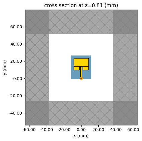
First, a cheap single-patch simulation checks the resonance and match. Closed-form patch formulas are typically accurate to 1–2 %. If the $S_{11}$ minimum misses 5.8 GHz, scale L_patch by $f_\mathrm{sim}/f_0$ and rerun this cell before simulating the array.
patch_layout, patch_modeler = make_antenna_modeler(1, directivity=False)
patch_modeler.plot_sim(z=h_sub)
plt.show()

patch_data = run_modeler(patch_modeler, "butler_single_patch")
S11_patch = sparams(patch_data).sel(port_in="ant1", port_out="ant1")
plt.plot(freqs / 1e9, 20 * np.log10(abs(S11_patch)))
plt.axvline(f0 / 1e9, color="gray", ls=":")
plt.xlabel("frequency (GHz)")
plt.ylabel("|S11| (dB)")
plt.grid(True)
plt.show()
f_res = float(freqs[np.argmin(abs(S11_patch.values))])
print(f"patch resonance: {f_res / 1e9:.3f} GHz")
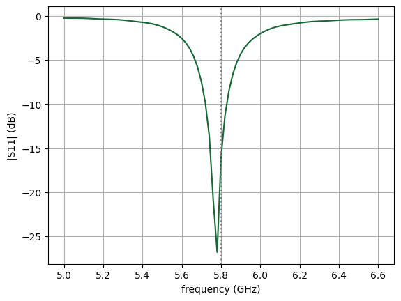
patch resonance: 5.780 GHz
Array Simulation
The TerminalComponentModeler excites each of the four array ports in turn while the other ports are terminated in 50 Ω, and records the radiated field of each excitation with the DirectivityMonitor. Mutual coupling between the elements is therefore fully included.
array_layout, array_modeler = make_antenna_modeler(4)
fig, ax = plt.subplots(figsize=(10, 5))
array_modeler.plot_sim(z=h_sub, ax=ax)
plt.show()
print(f"grid cells: {array_modeler.simulation.num_cells / 1e6:.2f} M")
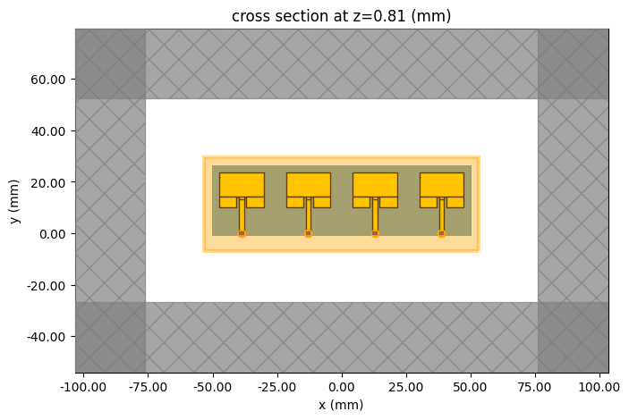
grid cells: 4.31 M
array_data = run_modeler(array_modeler, "butler_patch_array_1x4")
Step 5: Switched Beams
Because the system is linear, the field radiated when the Butler matrix is driven at input i is a superposition of the four per-port array patterns. Each pattern is weighted by the incident wave that the matrix delivers to that element, $a_k = S_{\mathrm{out}_k,\mathrm{in}_i}$. The modeler data does this combination for us through the port_amplitudes argument of get_antenna_metrics_data.
This cascade assumes that the matrix outputs and the array inputs are both well matched to 50 Ω. Multiple reflections between the two networks are neglected, which is accurate when both return losses are better than about 15 dB. For comparison, we also show the ideal array factor $AF(\theta) = \left|\sum_k a_k e^{-ik_0 x_k\sin\theta}\right|^2$ computed from the circuit-model amplitudes and scaled to the simulated peak gain.
x_elem = (np.arange(4) - 1.5) * d_elem
theta_plot = np.linspace(-90, 90, 361)


def pattern_xz(metrics, quantity="realized_gain"):
    """Extract a pattern in the xz-plane (phi=0 for theta>0, phi=pi for theta<0) in dB."""
    g = getattr(metrics, quantity).sel(f=f0, method="nearest").squeeze(drop=True)
    th = np.rad2deg(g.theta.values)
    right = g.sel(phi=0.0, method="nearest").values
    left = g.sel(phi=np.pi, method="nearest").values
    ang = np.concatenate([-th[::-1], th])
    val = np.concatenate([left[::-1], right])
    keep = abs(ang) <= 90
    return ang[keep], 10 * np.log10(np.maximum(val[keep], 1e-6))


fig, ax = plt.subplots(figsize=(9, 5))
summary = []
for c, i_name in enumerate(IN):
    amps = {f"ant{k + 1}": complex(T_fdtd[k, c]) for k in range(4)}
    metrics = array_data.get_antenna_metrics_data(
        port_amplitudes=amps, monitor_name="directivity"
    )
    ang, gain_db = pattern_xz(metrics)
    (l,) = ax.plot(ang, gain_db, label=f"{i_name} (FDTD)")
    # ideal array factor from the circuit model, normalised to the simulated peak
    af = (
        abs(
            np.exp(-1j * k0 * np.outer(np.sin(np.deg2rad(theta_plot)), x_elem))
            @ T_c[:, c]
        )
        ** 2
    )
    ax.plot(
        theta_plot,
        10 * np.log10(af / af.max()) + gain_db.max(),
        "--",
        color=l.get_color(),
        lw=1,
    )
    summary.append((i_name, ang[np.argmax(gain_db)], gain_db.max()))

ax.set_ylim(gain_db.max() - 25, gain_db.max() + 3)
ax.set_xlabel("theta in xz-plane (deg)")
ax.set_ylabel("realized gain (dBi)")
ax.set_title("Switched beams at 5.8 GHz: FDTD (solid) vs array factor (dashed)")
ax.grid(True)
ax.legend()
plt.show()

print(f"{'input':>6} {'beam (deg)':>11} {'theory (deg)':>13} {'peak gain (dBi)':>16}")
for (i_name, th_pk, g_pk), c in zip(summary, range(4)):
    th_theory = np.rad2deg(np.arcsin(np.deg2rad(dphi_c[:, c].mean()) / (k0 * d_elem)))
    print(f"{i_name:>6} {th_pk:11.1f} {th_theory:13.1f} {g_pk:16.2f}")
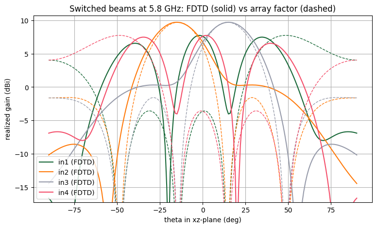
 input  beam (deg)  theory (deg)  peak gain (dBi)
   in1        -2.0          48.6             7.75
   in2       -15.0         -14.5             9.71
   in3        15.0          14.5             9.71
   in4         2.0         -48.6             7.74
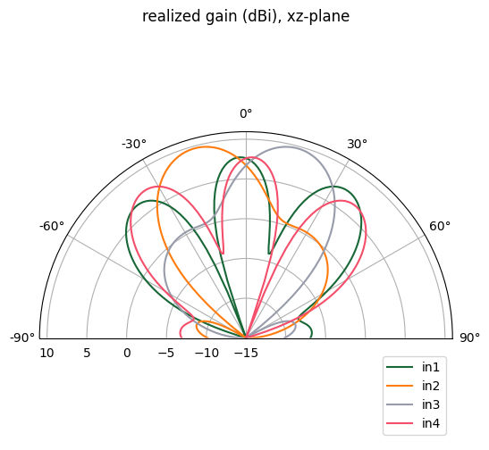
Polar View of the Four Beams
fig = plt.figure(figsize=(6, 6))
axp = fig.add_subplot(projection="polar")
for c, i_name in enumerate(IN):
    amps = {f"ant{k + 1}": complex(T_fdtd[k, c]) for k in range(4)}
    metrics = array_data.get_antenna_metrics_data(
        port_amplitudes=amps, monitor_name="directivity"
    )
    ang, gain_db = pattern_xz(metrics)
    axp.plot(np.deg2rad(ang), np.maximum(gain_db, -15), label=i_name)
axp.set_theta_zero_location("N")
axp.set_theta_direction(-1)
axp.set_thetamin(-90)
axp.set_thetamax(90)
axp.set_rlim(-15, None)
axp.legend(loc="lower right")
axp.set_title("realized gain (dBi), xz-plane")
plt.show()
Summary
We designed a complete 5.8 GHz switched-beam antenna system:
- The layout-aware circuit model sized the 45° and 0° compensation lines from the same geometry description used for the full-wave models, with no hand calculation of electrical lengths.
- The
TerminalComponentModelerwithLumpedPorts verified the branch-line hybrid, the 0 dB crossover and the complete 8-port Butler matrix.run_onlylimited the number of simulations to the excitations that are actually needed. - Combining the simulated 1×4 patch array with the simulated Butler-matrix outputs through
port_amplitudesproduced the four switched beams near ±14.5° and ±48.6°, in good agreement with array theory.
Natural extensions of this notebook:
- Include conductor loss and surface roughness with
td.LossyMetalMedium, and compare the insertion loss with the lossless case. - Simulate the matrix and the array together on one board. This captures the interaction between the two networks directly and removes the need for the cascade approximation.
- Use the autograd plugin to optimise the hybrid arm widths and lengths for wider bandwidth.
- Scale the same
Layoutgenerator to an 8×8 Butler matrix (12 hybrids, 16 crossovers).


 TERMS & CONDITIONS


 How the process works:
 Try this real URL to see an example: