Author: Conganige Anthony, Queen's University
As silicon photonic technologies mature, many platforms direct their attention towards minimizing loss throughout their circuit. A major proponent of this is the loss introduced from bends. In this notebook, we recreate the work of Deng et al., entitled "Low-loss Waveguide Bend Supporting a Whispering Gallery Mode," Silicon Photonics Conference (SiPhotonics), 2023. DOI: https://10.1109/SiPhotonics55903.2023.10141913 where they demonstrate the loss of their proposed bends relative to other conventional bending shapes.
Overview
To do this, we set up simulations for a circular and Poly3 (this work) curve. Then, we run full 3D FDTD simulations of each with an effective radius of 15um and compare the loss across each device. The circular bend is taken from this example notebook on the Tidy3D website.
Set up Simulation
# Import relevant libraries
import numpy as np
import tidy3d as td
import tidy3d.web as web
from shapely.geometry import Polygon as ShapelyPolygon
import gdstk
import matplotlib.pyplot as plt
import scipy.integrate as integrate
from scipy.optimize import fsolve
from scipy.optimize import brentq
# Define simulation parameters
wl0 = 0.638
freq0 = td.C_0 / wl0
fwidth = 0.2 * freq0
npoints = 100
freqs = np.linspace(freq0 - fwidth / 2, freq0 + fwidth / 2, npoints)
run_time = 1e-12

# Define material properties
n_SiN = 2.038
n_SiO2 = 1.4569
SiN = td.Medium(permittivity=n_SiN**2)
SiO2 = td.Medium(permittivity=n_SiO2**2)

# Define geometric parameters
h_SiN = 0.15
W_wg = 0.5
R = 15 # effective bend radius
theta_t = np.pi / 2 # total bend angle
L_str = 3.0 # straight input/output section length
inf = 100
A = 2.4
buffer = 1
Necessary helper functions for generating the different curve types, and for eventual post-processing
# Poly3 Functions
def poly3_theta(s, Rc, tt, tc):
    """Tangential angle along Poly3 (Eq. 1)."""
    return (2 * Rc * (tt - tc) * s**3 - s**4) / (2 * Rc**4 * (tt - tc)**3)


def _poly3_endpoint(Rc, tt, tc, n=3000):
    """Integrate (cos, sin) to find the Poly3 endpoint."""
    s = np.linspace(0, Rc * (tt - tc), n)
    th = poly3_theta(s, Rc, tt, tc)
    return np.trapezoid(np.cos(th), s), np.trapezoid(np.sin(th), s)


def _constraint(Rc, R, tt, tc):
    """Bisector symmetry constraint (Eq. 2)."""
    px, py = _poly3_endpoint(Rc, tt, tc)
    ang = (tt - tc) / 2
    xo = px - Rc * np.sin(ang)
    yo = py + Rc * np.cos(ang)
    return xo * np.cos(tt / 2) + (yo - R) * np.sin(tt / 2)


def find_Rc(R, tt, tc):
    """Solve for the Circ arc radius Rc given (R, theta_t, theta_c)."""
    return brentq(_constraint, 1e-4 * R, 10 * R, args=(R, tt, tc))


def generate_baseline(R, tt, tc, n=1200):
    """
    Build the Poly3 + Circ + Poly3' centreline.
    Starts at (0, 0) heading in +x; ends at (R, R) heading in +y (for theta_t = pi/2).
    """
    Rc  = find_Rc(R, tt, tc)
    L_p = Rc * (tt - tc)

    # Poly3
    n_p  = n // 3
    s_p  = np.linspace(0, L_p, n_p)
    th_p = poly3_theta(s_p, Rc, tt, tc)
    xp   = np.concatenate([[0.0], np.cumsum(np.cos(th_p[:-1]) * np.diff(s_p))])
    yp   = np.concatenate([[0.0], np.cumsum(np.sin(th_p[:-1]) * np.diff(s_p))])

    # Circ arc
    ang     = (tt - tc) / 2
    xo      = xp[-1] - Rc * np.sin(ang)
    yo      = yp[-1] + Rc * np.cos(ang)
    n_c     = n // 3
    a_start = np.arctan2(yp[-1] - yo, xp[-1] - xo)
    alphas  = np.linspace(a_start, a_start + tc, n_c)
    xc      = xo + Rc * np.cos(alphas)
    yc      = yo + Rc * np.sin(alphas)

    # Poly3' (mirror of Poly3)
    n_pp  = n - n_p - n_c + 2
    s_pp  = np.linspace(0, L_p, n_pp)
    th_pp = tt - poly3_theta(L_p - s_pp, Rc, tt, tc)
    xpp   = np.concatenate([[xc[-1]], xc[-1] + np.cumsum(np.cos(th_pp[:-1]) * np.diff(s_pp))])
    ypp   = np.concatenate([[yc[-1]], yc[-1] + np.cumsum(np.sin(th_pp[:-1]) * np.diff(s_pp))])

    return (np.concatenate([xp, xc[1:], xpp[1:]]),
            np.concatenate([yp, yc[1:], ypp[1:]]))


def offset_curve(x, y, d):
    """
    Offset a curve by signed distance d along its left-pointing normal.
    d > 0 -> inward (toward centre of curvature)
    d < 0 -> outward
    """
    dx, dy = np.gradient(x), np.gradient(y)
    mag    = np.hypot(dx, dy) + 1e-30
    return x + d * (-dy / mag), y + d * (dx / mag)

# Euler Functions
def euler_curve(L_max, A, num_points=50):
    Ls = np.linspace(0, L_max, num_points)

    y1 = np.array([integrate.quad(lambda theta: A * np.sin(theta**2 / 2), 0, L / A)[0] for L in Ls])
    x1 = np.array([integrate.quad(lambda theta: A * np.cos(theta**2 / 2), 0, L / A)[0] for L in Ls])

    return x1, y1

def calculate_L_max(R_eff, A, num_points=50, tolerance=1e-12):
    def func(L_max):
        L_max = float(L_max.item())
        x1, y1 = euler_curve(L_max, A, num_points)

        # compute the derivative at L_max
        k = -(x1[-1] - x1[-2]) / (y1[-1] - y1[-2])
        xp = x1[-1]
        yp = y1[-1]

        # check if the derivative is continuous at L_max
        R = np.sqrt(
            ((R_eff + k * xp - yp) / (k + 1) - xp) ** 2
            + (-(R_eff + k * xp - yp) / (k + 1) + R_eff - yp) ** 2
        )
        return np.abs(R - A**2 / L_max)

    res = fsolve(func, x0=(1,), full_output=True)

    error = res[1]["fvec"]

    if error > tolerance:
        raise ValueError(f"No solutions for given A: {A}.")
    L_max = res[0][0]

    return L_max

L_max = calculate_L_max(R, A)

x1, y1 = euler_curve(L_max, A)

xp = x1[-1]
yp = y1[-1]

R_min = A**2 / L_max

# Circular Functions
def circle(var):
    a = var[0]
    b = var[1]
    Func = np.empty(2)
    Func[0] = (xp - a) ** 2 + (yp - b) ** 2 - R_min**2
    Func[1] = (R - yp - a) ** 2 + (R - xp - b) ** 2 - R_min**2
    return Func

def mirror_path(x_points, y_points, mirror_y=0):
    y_mirrored = 2 * mirror_y - y_points
    return x_points, y_mirrored

def line_to_structure(x, y, w, t):
    cell = gdstk.Cell("bend")  # define a gds cell

    # add points to include the input and output straight waveguides

    cell.add(gdstk.FlexPath(x + 1j * y, w, layer=1, datatype=0))  # add path to cell

    # define structure from cell
    bend = td.Structure(
        geometry=td.PolySlab.from_gds(
            cell,
            gds_layer=1,
            axis=2,
            slab_bounds=(-t/2, t/2),
        )[0],
        medium=SiN,
    )

    return bend

def poly_slab(verts, med):
    return td.Structure(
        geometry=td.PolySlab(vertices=verts, slab_bounds=(-h_SiN/2, h_SiN/2), axis=2, sidewall_angle=np.radians(0)),
        medium=med,
    )

# Visualization Functions
def plot_conversion_efficiency(sim_data, mon_name=["mode"], labels=[], title="", show=True):
    # extract the conversion efficiency from the mode monitor
    for mon in mon_name:
        amp = sim_data[mon].amps.sel(mode_index=0, direction="-")
        freq = sim_data[mon].amps.f
        wl = td.C_0 / freq
        T = np.abs(amp) ** 2
        plt.plot(wl, -10*np.log10(np.abs(T)**2), label=labels[mon_name.index(mon)])

    plt.xlim(0.613, 0.663)
    plt.xlabel(r"Wavelength ($\mu m$)")
    plt.ylabel("Bending Loss (dB)")
    plt.legend()
    plt.title(title)
    if show:
        plt.show()

def plot_field(sim_data):

    ax = sim_data.plot_field(
        field_monitor_name="field", field_name="E", val="abs", f= freq0, vmin=0, vmax=100,
    )
    plt.show()
Define the simulation object
# input/output waveguides
input_waveguide = td.Structure(
geometry=td.Box(
center=(-1, 0, 0),
size=(L_str, W_wg, h_SiN),
),
medium=SiN,
)
output_waveguide = td.Structure(
geometry=td.Box(
center=(-1, 2*R, 0),
size=(L_str, W_wg, h_SiN),
),
medium=SiN,
)
# add a mode source that launches the fundamental te mode
mode_spec = td.ModeSpec(num_modes=1, target_neff=n_SiN)
mode_source = td.ModeSource(
center=(-buffer, 0, 0),
size=(0, 4 * W_wg, 6 * h_SiN),
source_time=td.GaussianPulse(freq0=freq0, fwidth=fwidth),
direction="+",
mode_spec=mode_spec,
mode_index=0,
)
# add a mode monitor to measure transmission
mode_monitor = td.ModeMonitor(
center=(0, 2*R, 0),
size=(0, 4 * W_wg, 6 * h_SiN),
freqs=freqs,
mode_spec=mode_spec,
name="mode",
)
# add a field monitor to visualize field propagation and leakage in the bend
field_monitor = td.FieldMonitor(
center=(R, R + buffer, 0),
size=(td.inf, td.inf, 0),
freqs=[freq0],
colocate=True,
name="field",
)
# define simulation
sim = td.Simulation(
center=(R/2, R, 0),
size=(2*R-12, 2*R + 2 * W_wg + wl0+1, 10 * h_SiN),
grid_spec=td.GridSpec.auto(min_steps_per_wvl=20, wavelength=wl0),
structures=[input_waveguide, output_waveguide],
sources=[mode_source],
monitors=[mode_monitor, field_monitor],
run_time=run_time,
boundary_spec=td.BoundarySpec.all_sides(boundary=td.PML()), # pml is applied in all boundaries
medium=SiO2,
symmetry = (0, 0, 1) # apply mirror symmetry in z direction to reduce simulation cost
) # background medium is set to sio2 because of the substrate and upper cladding
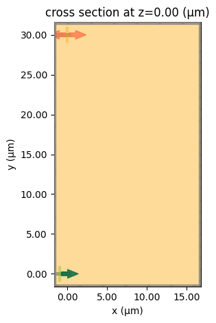
sim.plot(z=0)
plt.show()
Loss of a Circular Bend
We begin with a circular bend, setting up the simulation object using our pre-defined helper functions.
a, b = fsolve(circle, (0, R))

# calculate the coordinates of the circular curve
x2 = np.linspace(xp + 0.01, R - yp - 0.01, 50)
y2 = -np.sqrt(R_min**2 - (x2 - a) ** 2) + b

x_circle = np.linspace(0, R, 100)
y_circle = -np.sqrt(R**2 - (x_circle) ** 2) + R
x4, y4 = mirror_path(x_circle, y_circle, mirror_y=R)

x = np.concatenate([x_circle, x4[::-1]])
y = np.concatenate([y_circle, y4[::-1]])

# # create the circular bend geometry
circular_bend = line_to_structure(x, y, W_wg, h_SiN)
# add the circular bend to the simulation
sim_circular = sim.updated_copy(structures=[input_waveguide, output_waveguide, circular_bend])

# visualize the circular bend structure
sim_circular.plot(z=0)
<Axes: title={'center': 'cross section at z=0.00 (μm)'}, xlabel='x (μm)', ylabel='y (μm)'>
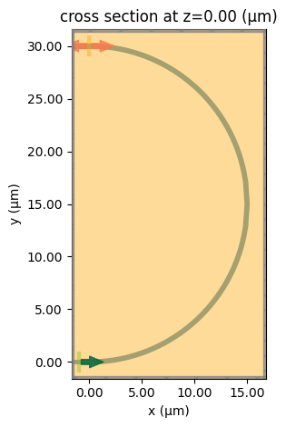
Now that we have confirmed that our simulation is properly set up, we can calculate the loss of the curve by running the FDTD simulation.
sim_data_circular = web.run(sim_circular, "circular_bend", verbose=True)
10:53:48 EDT Created task 'circular_bend' with resource_id
             'fdve-54560c3e-c982-4f45-8527-1767825ad30b' and task_type 'FDTD'.
             View task using web UI at
             'https://tidy3d.simulation.cloud/workbench?taskId=fdve-54560c3e-c98
             2-4f45-8527-1767825ad30b'.
Task folder: 'default'.
Output()
10:53:50 EDT Estimated FlexCredit cost: 1.272. Minimum cost depends on task
             execution details. Use 'web.real_cost(task_id)' to get the billed
             FlexCredit cost after a simulation run.
10:53:51 EDT status = success
Output()
10:53:57 EDT Loading results from simulation_data.hdf5
Now to visualize the results
plot_conversion_efficiency(sim_data_circular, mon_name=["mode"], labels=["circular bend"], title="Bending Loss of Circular Bend")
plot_field(sim_data_circular)
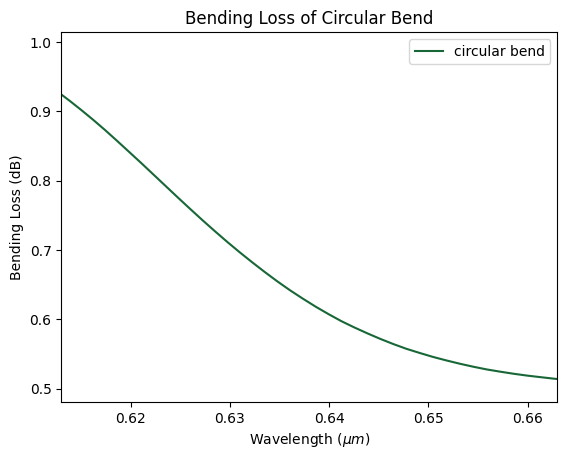
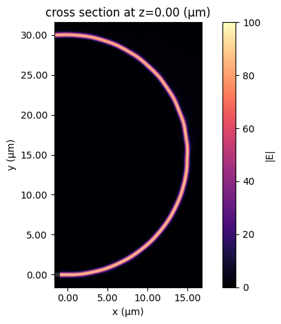
While not terrible, the bending losses of the circular curve leaves much to be desired, which is why we turn our attention next to the Poly3 bend.
Loss of a Poly3 Bend
In their paper, Deng et al. give us the following:
A Poly3 bend is defined by a Poly3 segment, a circular segment, and then a Poly3' segment. To calculate the coordinates for a Poly3 segment, we follow the equation $$(x(l),y(l))=\int_{0}^{l}(\cos\theta,\sin\theta)ds,\quad\text{for }0\leq l\leq R_{c}(\theta_{t}-\theta_{c}),$$ where $R_{c}$ is the circular bend radius, with angle $\theta_{c}$, $\theta_{t}$ is the angle of the equivalent circular arc, and $$\theta(s)=\frac{2R_{c}(\theta_{t}-\theta_{c}s^{3}-s^{4})}{2R_{c}^{4}(\theta_{t}-\theta_{c})^{3}}.$$ The circular segment is generated as a circular bend with center ($x_{0}, y_{0}$), radius $R_{c}$, and angle $\theta_{c}$ with the constraints: $$\begin{cases}x_{0}\cos\frac{\theta_{t}}{2}+(y_{0}-R)\sin\frac{\theta_{t}}{2}=0\\ x_{0}=\int_{0}^{R_{c}(\theta_{t}-\theta_{c})}\cos\theta ds-R_{c}\sin\frac{\theta_{t}-\theta_{c}}{2}\\ y_{0}=\int_{0}^{R_{c}(\theta_{t}-\theta_{c})}\sin\theta ds+R_{c}\cos\frac{\theta_{t}-\theta_{c}}{2}\end{cases}.$$ Finally, the Poly3' segment is formed by mirroring the Poly3 segment about the bisector of $\theta_{t}.$
All of these have been implemented in the helper functions defined previously, so now we generate our geometry and simulate it.
theta_t = np.pi
theta_c_outer = 2 * np.pi / 3
theta_c_inner = 2 * np.pi / 3
x_outer, y_outer = generate_baseline(R, theta_t, theta_c_outer)
x_inner, y_inner = generate_baseline(R, theta_t, theta_c_inner)
# Outer wall: outer baseline shifted outward by W_wg/2
x_wall_out, y_wall_out = offset_curve(x_outer, y_outer, -W_wg / 2)
# Inner wall: inner baseline shifted inward by W_wg/2
x_wall_inn, y_wall_inn = offset_curve(x_inner, y_inner, +W_wg / 2)
# Close polygon: outer boundary forward, inner boundary backward
bend_verts = list(zip(
np.concatenate([x_wall_out, x_wall_inn[::-1]]).tolist(),
np.concatenate([y_wall_out, y_wall_inn[::-1]]).tolist(),
))
bend_verts = list(ShapelyPolygon(bend_verts).simplify(1e-3).exterior.coords[:-1])
bend = poly_slab(bend_verts, SiN)
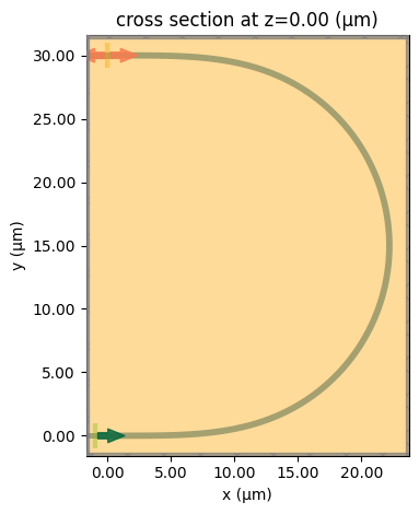
sim_poly = sim.updated_copy(structures=[input_waveguide, output_waveguide, bend], size=(2*R-5, 2*R + 2 * W_wg + wl0+1, 10 * h_SiN), center=(R-4, R, 0))
sim_poly.plot(z=0)
<Axes: title={'center': 'cross section at z=0.00 (μm)'}, xlabel='x (μm)', ylabel='y (μm)'>
sim_data_poly = web.run(sim_poly, "poly_bend", verbose=False)
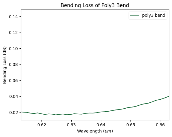
plot_conversion_efficiency(sim_data_poly, mon_name=["mode"], labels=["poly3 bend"], title="Bending Loss of Poly3 Bend")
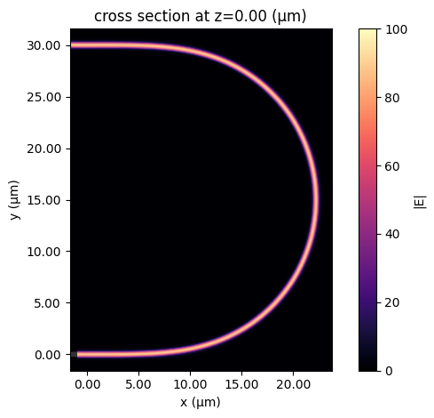
plot_field(sim_data_poly)
Comparison
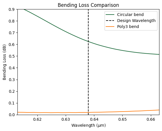
Now we overlap the two bending loss plots to confirm the performance of the low-loss bend
plot_conversion_efficiency(sim_data_circular, mon_name=["mode"], labels=["Circular bend"], title="Bending Loss of Circular Bend", show=False)
plt.vlines(x=wl0, ymin=0, ymax=0.9, color='k', linestyle='--', label='Design Wavelength')
plt.ylim(0,0.9)
plot_conversion_efficiency(sim_data_poly, mon_name=["mode"], labels=["Poly3 bend"], title="Bending Loss Comparison", show=True)
Conclusion
Here, we demonstrated a new type of bend proposed by Deng et al. which has significantly lower bending loss compared to a traditional circular bend. While being slightly larger than a circular bend, the loss advantage gives promise for applications across the field of integrated photonics.