Author: Helaman Flores, MIT
Four-wave mixing (FWM) is a third-order ($\chi^{(3)}$) nonlinear optical process in which two pump photons are converted into a signal and an idler photon, satisfying both energy and momentum conservation:
$$\omega_\text{signal} + \omega_\text{idler} = \omega_{\text{pump}_A} + \omega_{\text{pump}_B}$$
In a ring resonator, momentum conservation reduces to an integer condition on the azimuthal mode numbers $m$:
$$m_\text{signal} + m_\text{idler} = m_{\text{pump}_A} + m_{\text{pump}_B}$$
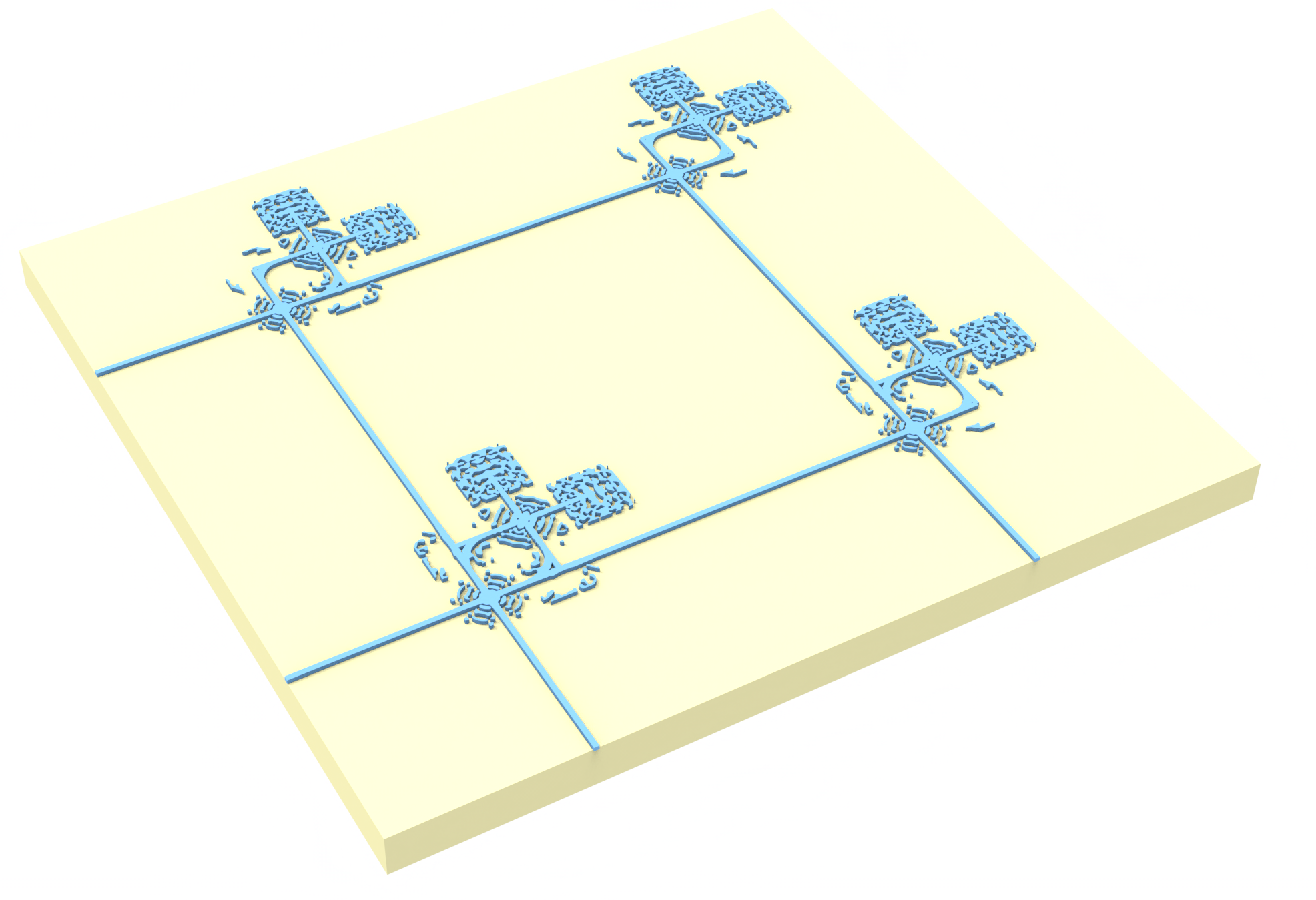
This notebook models a diamond ring resonator on a Si₃N₄/SiO₂ substrate. Diamond combines a large $\chi^{(3)}$ coefficient, wide transparency window (UV to mid-IR), and negligible two-photon absorption at telecom wavelengths.
The workflow proceeds in four stages:
- Effective index sweep — compute waveguide dispersion across widths and frequencies using the ModeSolver.
- Phase-matching selection — identify azimuthal mode-number quartets that simultaneously satisfy energy and momentum conservation.
- Resonance locking — run FDTD simulations with a ResonanceFinder monitor to precisely locate each resonance.
- Efficiency estimation — compute the $\chi^{(3)}$ polarization overlap and extract the idler quality factor $Q$ and mode volume $V$.
For a simpler introduction to $\chi^{(3)}$ FWM in Tidy3D, see Generation of Kerr sideband.
FDTD simulations can diverge due to various reasons. If you encounter any simulation divergence issues, follow the steps in our troubleshooting guide.
Imports
import xarray as xr
import numpy as np
from numpy.polynomial import Polynomial

import tidy3d as td
from tidy3d.plugins.dispersion import AdvancedFastFitterParam, FastDispersionFitter
from tidy3d.plugins.resonance import ResonanceFinder
from tidy3d.plugins.mode import ModeSolver
from tidy3d.components.simulation import AbstractYeeGridSimulation
from tidy3d.components.structure import Structure
from tidy3d.components.grid.grid import Grid, Coords
import matplotlib.cm as cm
import matplotlib.pyplot as plt
from scipy.constants import c

from tqdm import tqdm

td.config.logging_level = "ERROR"
Utilities
Helper functions and classes for running generic ring resonator simulations and computing the effective mode index.
def get_fdtd_sim(
    simulation,
    ports,
    freqs,
    layer_z_centers,
    inputs,
    outputs,
    mode_volume=None,
    farfield=None,
    flux=None,
    output_freqs=None,
    custom_sources=None,
    sim_kwargs=None,
):
    """Returns the FDTD simulation object for a given set of inputs and outputs.

    Args:
        simulation: base td.Simulation (structures + domain, no sources/monitors)
        ports: dict of port info, e.g.
            {'o1': {'center': (x,y,z), 'size': (sx,sy,sz),
                    'direction': '+'/'-', 'mode_spec': td.ModeSpec}}
        freqs: array of frequencies used to compute default bandwidth
        layer_z_centers: dict {'diamond': z_value, ...} for field monitor positioning
        inputs: dict{port_name: {modes, amps, phases, freqs, fwidths}}
        outputs: dict{port_name: {types: list[str]}}
        mode_volume: dict with keys 'layer', 'thickness', 'downsample', etc.
        farfield: dict with keys 'downsample', 'surface', 'res', etc.
        flux: dict with keys 'downsample', 'apodization', etc.
        output_freqs: list of floats
        custom_sources: list of custom td sources
        sim_kwargs: dict of kwargs passed to simulation update
    """
    sources = []
    if custom_sources is not None:
        if not isinstance(custom_sources, list):
            custom_sources = [custom_sources]
        sources.extend(custom_sources)
    monitors = []
    if sim_kwargs is None:
        sim_kwargs = {}

    # Validate port names
    port_names = set(list(inputs.keys()) + list(outputs.keys()))
    missing_ports = port_names - set(ports.keys())
    if missing_ports:
        raise ValueError(f"Ports {missing_ports} not found in ports dict")
    if output_freqs is None:
        output_freqs = np.mean(freqs)

    for port_name, port_info in ports.items():
        p_center = port_info["center"]
        p_size = port_info["size"]
        p_direction = port_info["direction"]
        p_mode_spec = port_info["mode_spec"]

        if port_name in inputs:
            inp = inputs[port_name]
            if "freqs" not in inp:
                inp["freqs"] = [None] * len(inp["modes"])
            if "fwidths" not in inp:
                inp["fwidths"] = [None] * len(inp["modes"])
            if "port_offset" not in inp:
                inp["port_offset"] = [(0, 0, 0)] * len(inp["modes"])
            for (
                input_mode,
                input_amp,
                input_phase,
                input_freq,
                input_fwidth,
                input_port_offset,
            ) in zip(
                inp["modes"],
                inp["amps"],
                inp["phases"],
                inp["freqs"],
                inp["fwidths"],
                inp["port_offset"],
            ):
                if isinstance(input_mode, str) and ("dipole" in input_mode):
                    freq0 = input_freq if input_freq is not None else np.mean(freqs)
                    if input_fwidth is None:
                        fdiff = max(freqs) - min(freqs)
                        fwidth = max(fdiff, max(output_freqs) / 10)
                    else:
                        fwidth = input_fwidth
                    dipole_source = td.PointDipole(
                        center=(
                            p_center[0] + input_port_offset[0],
                            p_center[1] + input_port_offset[1],
                            p_center[2] + input_port_offset[2],
                        ),
                        source_time=td.GaussianPulse(
                            freq0=freq0,
                            fwidth=fwidth,
                            phase=input_phase,
                            amplitude=input_amp,
                        ),
                        name=port_name
                        + f"@{input_mode}"
                        + (f"@{input_freq}" if input_freq is not None else ""),
                        polarization=input_mode.split("_")[1],
                    )
                    sources.append(dipole_source)
                else:
                    freq0 = input_freq if input_freq is not None else np.mean(freqs)
                    if input_fwidth is None:
                        fdiff = max(freqs) - min(freqs)
                        fwidth = max(fdiff, freq0 * 0.1)
                    else:
                        fwidth = input_fwidth
                    source_time = td.GaussianPulse(
                        freq0=freq0,
                        fwidth=fwidth,
                        amplitude=input_amp,
                        phase=input_phase,
                    )
                    mode_source = td.ModeSource(
                        center=p_center,
                        size=p_size,
                        source_time=source_time,
                        mode_spec=p_mode_spec,
                        mode_index=input_mode,
                        direction=p_direction,
                        name=port_name,
                    )
                    sources.append(mode_source)

        if port_name in outputs:
            if len(outputs[port_name]["types"]) == 0:
                outputs[port_name]["types"] = ["mode"]
            for output_type in outputs[port_name]["types"]:
                if output_type == "mode":
                    output_monitor = td.ModeMonitor(
                        center=p_center,
                        size=p_size,
                        freqs=output_freqs
                        if isinstance(output_freqs, (list, np.ndarray))
                        else [output_freqs],
                        mode_spec=p_mode_spec,
                        name=port_name,
                    )
                elif "time" in output_type:
                    fdiff = max(freqs) - min(freqs)
                    fwidth = max(fdiff, max(output_freqs) / 10)
                    t_start = 2 / fwidth
                    output_monitor = td.FieldTimeMonitor(
                        fields=[output_type.split("_")[1]],
                        center=p_center,
                        size=(0, 0, 0),
                        start=t_start,
                        name=port_name + "_" + output_type,
                    )
                monitors.append(output_monitor)

    sim_center = simulation.center
    sim_size = sim_kwargs.get("size", simulation.size)
    if mode_volume is not None:
        if "downsample" not in mode_volume or mode_volume["downsample"] is None:
            mode_volume["downsample"] = (4, 4, 2)
        if "apodization" in mode_volume:
            apod_spec = td.ApodizationSpec(
                start=mode_volume["apodization"]["start"],
                width=mode_volume["apodization"]["width"],
            )
        else:
            apod_spec = td.ApodizationSpec()
        if "colocate" in mode_volume:
            colocate = mode_volume["colocate"]
        else:
            colocate = True
        monitors.append(
            td.FieldMonitor(
                name="field",
                center=[0, 0, layer_z_centers[mode_volume["layer"]]],
                size=[td.inf, td.inf, mode_volume["thickness"]],
                interval_space=mode_volume["downsample"],
                freqs=output_freqs
                if isinstance(output_freqs, (list, np.ndarray))
                else [output_freqs],
                apodization=apod_spec,
                colocate=colocate,
            )
        )
    if farfield is not None:
        if "downsample" not in farfield or farfield["downsample"] is None:
            farfield["downsample"] = (4, 4, 4)
        if "apodization" in farfield:
            apod_spec = td.ApodizationSpec(
                start=farfield["apodization"]["start"],
                width=farfield["apodization"]["width"],
            )
        else:
            apod_spec = td.ApodizationSpec()
        distance_from_pml = 0.1
        if "surface" not in farfield or farfield["surface"] == "spherical":
            thetas = farfield.get("thetas", np.linspace(0, np.pi, farfield["res"]))
            phis = farfield.get("phis", np.linspace(0, 2 * np.pi, 2 * farfield["res"]))
            exclude_surfaces = farfield.get("exclude_surfaces", None)
            monitors.append(
                td.FieldProjectionAngleMonitor(
                    name="farfield_monitor",
                    center=sim_center,
                    size=(
                        sim_size[0] - 2 * distance_from_pml,
                        sim_size[1] - 2 * distance_from_pml,
                        sim_size[2] - 2 * distance_from_pml,
                    ),
                    interval_space=farfield["downsample"],
                    freqs=output_freqs
                    if isinstance(output_freqs, (list, np.ndarray))
                    else [output_freqs],
                    theta=thetas,
                    phi=phis,
                    apodization=apod_spec,
                    exclude_surfaces=exclude_surfaces,
                )
            )
        elif farfield["surface"] == "cartesian":
            proj_distance = farfield.get("proj_distance", 1e6)
            res = farfield.get("res", 100)
            x = farfield.get(
                "x", np.linspace(-proj_distance / 2, proj_distance / 2, res)
            )
            y = farfield.get(
                "y", np.linspace(-proj_distance / 2, proj_distance / 2, res)
            )
            exclude_surfaces = farfield.get("exclude_surfaces", None)
            monitors.append(
                td.FieldProjectionCartesianMonitor(
                    name="farfield_monitor_cartesian",
                    center=sim_center,
                    size=(
                        sim_size[0] - 2 * distance_from_pml,
                        sim_size[1] - 2 * distance_from_pml,
                        sim_size[2] - 2 * distance_from_pml,
                    ),
                    interval_space=farfield["downsample"],
                    freqs=output_freqs
                    if isinstance(output_freqs, (list, np.ndarray))
                    else [output_freqs],
                    x=x,
                    y=y,
                    proj_axis=2,
                    proj_distance=proj_distance,
                    apodization=apod_spec,
                    exclude_surfaces=exclude_surfaces,
                )
            )
    if flux is not None:
        if "downsample" not in flux or flux["downsample"] is None:
            flux["downsample"] = (4, 4, 4)
        if "apodization" in flux:
            apod_spec = td.ApodizationSpec(
                start=flux["apodization"]["start"], width=flux["apodization"]["width"]
            )
        else:
            apod_spec = td.ApodizationSpec()
        distance_from_pml = 0.1
        surfaces = {
            "left": "x-",
            "right": "x+",
            "back": "y-",
            "front": "y+",
            "bottom": "z-",
            "top": "z+",
        }
        for name, direction in surfaces.items():
            excludes = list({k: v for k, v in surfaces.items() if k != name}.values())
            monitors.append(
                td.FluxMonitor(
                    name="flux_" + name,
                    center=sim_center,
                    size=(
                        sim_size[0] - 2 * distance_from_pml,
                        sim_size[1] - 2 * distance_from_pml,
                        sim_size[2] - 2 * distance_from_pml,
                    ),
                    interval_space=flux["downsample"],
                    freqs=output_freqs
                    if isinstance(output_freqs, (list, np.ndarray))
                    else [output_freqs],
                    apodization=apod_spec,
                    exclude_surfaces=excludes,
                )
            )

    sim = simulation.updated_copy(sources=sources, monitors=monitors, **sim_kwargs)
    return sim
class NeffMixer:
def __init__(self, freqs, neffs, num_modes, layer_widths, layer_height, meta_data):
"""Initializes a NeffMixer object.
inputs:
freqs (Nx1 array): list of frequencies
neffs (WxNxM array): list of effective indices
num_modes (int): M, the number of modes
layer_widths (Wx1 array): list of widths for the chosen layer
layer_height (float): height of the chosen layer
meta_data (dict(str, any)): dictionary of meta data
"""
self.freqs = freqs
self.neffs = neffs
self.num_modes = num_modes
self.layer_widths = layer_widths
self.layer_height = layer_height
self.meta_data = meta_data
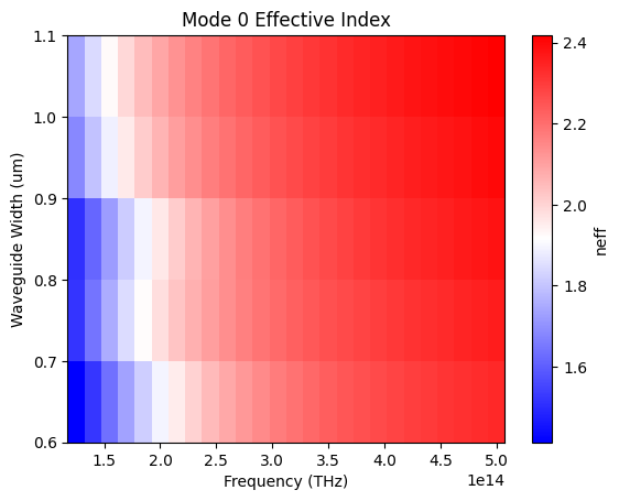
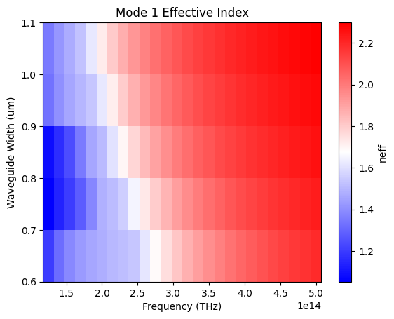
def plot(self, mode_num=0):
freqs_grid, wg_widths_grid = np.meshgrid(self.freqs, self.layer_widths)
plt.figure()
plt.pcolormesh(
freqs_grid,
wg_widths_grid,
self.neffs[:, :, mode_num],
shading="auto",
cmap="bwr",
)
plt.colorbar(label="neff")
plt.xlabel("Frequency (THz)")
plt.ylabel("Waveguide Width (um)")
plt.title(f"Mode {mode_num} Effective Index")
plt.show()
def net_momentum_matrix(
self,
fixed_freqs,
mode_factors,
mode_nums=0,
unit_ks=1,
fit_tol=1e-3,
poly_order=3,
plot=False,
num_freqs=100,
center_colorbar=False,
):
"""Returns the fwm net momentum matrix for mixing that targets the given output frequency.
inputs:
fixed_freqs ((K-2)x1 array): the frequencies of the fixed modes, where K is the number of modes involved in the mixing
mode_factors (Kx1 array): list of mode factors, where the last two are the mode factors of the independent and dependent modes, respectively
mode_nums (Kx1 array): list of mode numbers
unit_ks (Kx1 array): indicates the unit vector magnitude in the direction of net momentum
fit_tol (float): tolerance for the fit
plot (bool): whether to plot the net momentum matrix
outputs:
f_A (Vx1 array): the frequencies of the independent mode, where V is the number of valid frequencies
f_B (Vx1 array): the frequencies of the dependent mode, where V is the number of valid frequencies
net_momentum_matrix (WxV array): the net momentum matrix, where W is the number of widths and L is the number of valid frequencies
"""
if np.isscalar(mode_nums):
mode_nums = np.array([mode_nums] * len(mode_factors))
if np.isscalar(unit_ks):
unit_ks = np.array([unit_ks] * len(mode_factors))
if len(fixed_freqs) != len(mode_factors) - 2:
raise ValueError(
"The number of fixed frequencies must be equal to the number of modes minus 2"
)
if np.max(mode_nums) > self.num_modes:
raise ValueError(
f"The requested mode number ({np.max(mode_nums)}) is too high for the number of modes in the mixer ({self.num_modes})"
)
# Independent mode
min_freq = np.min(self.freqs)
max_freq = np.max(self.freqs)
f_A = np.linspace(min_freq, max_freq, num_freqs)
# Dependent mode
f_B = -mode_factors[-1] * (
np.sum(mode_factors[:-2] * fixed_freqs) + mode_factors[-2] * f_A
)
if plot:
plt.figure()
plt.plot(f_A / 1e12, f_B / 1e12)
plt.vlines(
[min_freq / 1e12, max_freq / 1e12],
min_freq / 1e12,
max_freq / 1e12,
color="k",
)
plt.hlines(
[min_freq / 1e12, max_freq / 1e12],
min_freq / 1e12,
max_freq / 1e12,
color="k",
)
plt.xlabel("Pump A Frequency (THz)")
plt.ylabel("Pump B Frequency (THz)")
plt.title("Pump Frequencies")
plt.legend(["Pumps", "Mixer Boundary"])
plt.show()
# Crop the frequencies to the range of the mixer
f_A = f_A[(f_B < np.max(self.freqs)) & (f_B > np.min(self.freqs))]
f_B = f_B[(f_B < np.max(self.freqs)) & (f_B > np.min(self.freqs))]
if len(f_A) == 0:
raise ValueError("No valid frequencies found for the mixer")
net_momentum_matrix = np.zeros((len(self.layer_widths), len(f_A)))
min_n_matrix = np.zeros((len(self.layer_widths), len(f_A)))
for w_i, width in enumerate(self.layer_widths):
k_fits = {}
n_fits = {}
for m_n in mode_nums:
if m_n not in k_fits:
n_fit, n_err = Polynomial.fit(
self.freqs, self.neffs[w_i, :, m_n], poly_order, full=True
)
n_fits[m_n] = n_fit
k_fits[m_n] = lambda f: 2 * np.pi * f / td.C_0 * n_fit(f)
if np.abs(n_err[0]) > fit_tol:
print(
f"Warning: n_err {np.abs(n_err[0][0]):.3e} is too large for mode {m_n}"
)
for m_n, n_fit in n_fits.items():
if w_i == 0 or w_i == len(self.layer_widths) - 1:
plt.plot(self.freqs, n_fit(self.freqs), label=f"Mode {m_n}")
plt.scatter(self.freqs, self.neffs[w_i, :, m_n])
if w_i == 0 or w_i == len(self.layer_widths) - 1:
plt.legend()
plt.show()
# Add the fixed modes to the net momentum matrix
fixed_iterable = zip(
mode_nums[:-2], fixed_freqs, mode_factors[:-2], unit_ks[:-2]
)
fixed_ks = np.array(
[
k_fits[mode_num](fixed_freq) * mode_factor * unit_k
for mode_num, fixed_freq, mode_factor, unit_k in fixed_iterable
]
)
net_momentum_matrix[w_i, :] = np.sum(fixed_ks)
# Add the independent mode to the net momentum matrix
independent_k = k_fits[mode_nums[-2]](f_A) * mode_factors[-2] * unit_ks[-2]
net_momentum_matrix[w_i, :] += independent_k
# Add the dependent mode to the net momentum matrix
dependent_k = k_fits[mode_nums[-1]](f_B) * mode_factors[-1] * unit_ks[-1]
net_momentum_matrix[w_i, :] += dependent_k
# Record the smallest effective index involved in the mixing
fixed_ns = np.array(
[
n_fits[mode_num](fixed_freq)
for mode_num, fixed_freq in zip(mode_nums[:-2], fixed_freqs)
]
)
independent_n = n_fits[mode_nums[-2]](f_A)
dependent_n = n_fits[mode_nums[-1]](f_B)
fixed_ns = np.tile(fixed_ns, (len(independent_n), 1))
all_ns = np.concatenate(
(fixed_ns, independent_n[:, np.newaxis], dependent_n[:, np.newaxis]),
axis=1,
)
min_n_matrix[w_i, :] = np.min(all_ns, axis=1)
if plot:
f_A_grid, widths_grid = np.meshgrid(f_A, self.layer_widths)
plt.figure()
if center_colorbar:
vmin = -np.max(np.abs(net_momentum_matrix))
vmax = np.max(np.abs(net_momentum_matrix))
else:
vmin = None
vmax = None
plt.pcolormesh(
f_A_grid / 1e12,
widths_grid,
net_momentum_matrix,
cmap="bwr",
shading="auto",
vmin=vmin,
vmax=vmax,
)
plt.title("Net Momentum Matrix")
plt.xlabel("Pump A Frequency (THz)")
plt.ylabel("Width (um)")
plt.colorbar()
plt.show()
plt.figure()
plt.pcolormesh(
f_A_grid / 1e12, widths_grid, min_n_matrix, cmap="hot", shading="auto"
)
plt.title("Minimum Effective Index Matrix")
plt.xlabel("Pump A Frequency (THz)")
plt.ylabel("Width (um)")
plt.colorbar()
plt.show()
return f_A, f_B, net_momentum_matrix, min_n_matrix
def scale_neffs(self, new_height, plot=False, plot_mode_num=0):
"""
Scale the frequencies and the widths to a new size, using the height of the layer at the given index
inputs:
new_height (float): the new height
"""
scale_factor = new_height / self.layer_height
self.layer_widths = self.layer_widths * scale_factor
self.layer_height = self.layer_height * scale_factor
self.freqs = self.freqs / scale_factor
if plot:
self.plot(plot_mode_num)
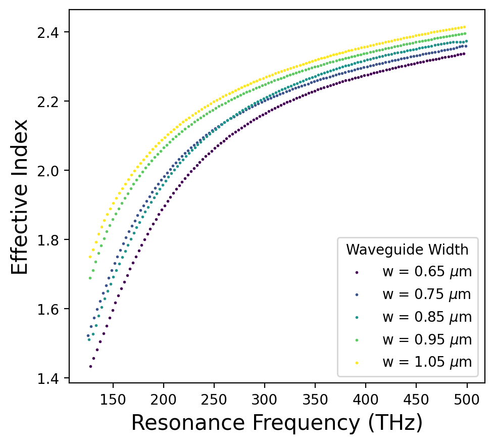
def get_resonances(
self, length, mode_num=0, plot=False, poly_order=3, fit_tol=2e-3
):
"""Returns the resonances for the given length
inputs:
length (float): the length of the resonator
outputs:
resonances (dict): Dictionary mapping width index to array of resonance frequencies and modes
resonances[w_i]['resonance_freqs'] (array): the resonance frequencies
resonances[w_i]['resonance_modes'] (array): the resonance modes
"""
# Calculate accumulated phase for each width and frequency
# Ensure self.freqs is a 1D array of frequencies (Hz)
freqs = np.array(self.freqs)
widths = np.array(self.layer_widths)
n_effs = np.array(self.neffs) # shape: (num_widths, num_freqs, num_modes)
# Only use the selected mode
n_effs_mode = n_effs[:, :, mode_num] # shape: (num_widths, num_freqs)
# Calculate wavelength for each frequency
wavelengths = c / freqs # shape: (num_freqs,)
# Calculate accumulated phase for each width and frequency
# shape: (num_widths, num_freqs)
accumulated_phase = (
2 * np.pi * n_effs_mode * length / wavelengths[np.newaxis, :]
)
# Mode number as a float
resonance_number = accumulated_phase / (
2 * np.pi
) # shape: (num_widths, num_freqs)
resonances = {}
if plot:
plt.figure(figsize=(5, 4.5), dpi=200)
colors = cm.viridis(np.linspace(0, 1, len(widths)))
for w_i, width in enumerate(widths):
# Find integer mode numbers within the range
min_mode = np.ceil(np.min(resonance_number[w_i, :]))
max_mode = np.floor(np.max(resonance_number[w_i, :]))
resonance_modes = np.arange(min_mode, max_mode + 1)
# Interpolate frequency at these integer mode numbers
interp_func, interp_err = Polynomial.fit(
resonance_number[w_i, :], freqs / 1e12, poly_order, full=True
)
if np.abs(interp_err[0]) > fit_tol:
print(
f"Warning: interp_err {np.abs(interp_err[0][0]):.3e} is too large for width {width:.2f} um"
)
resonance_freqs = interp_func(resonance_modes) * 1e12
resonances[w_i] = {}
resonances[w_i]["resonance_freqs"] = resonance_freqs
resonances[w_i]["resonance_modes"] = resonance_modes
if plot:
resonance_wavelengths = c / resonance_freqs
resonance_neffs = resonance_modes / length * resonance_wavelengths
plt.scatter(
resonance_freqs / 1e12,
resonance_neffs,
color=colors[w_i],
label=f"w = {width:.2f} $\\mu$m",
s=1,
)
# plt.plot(freqs/1e12, resonance_number[w_i, :], color=colors[w_i])
# plt.scatter(resonance_freqs / 1e12, resonance_modes, color=colors[w_i], label=f'Width={width:.2f} um', s=1)
if plot:
plt.xlabel("Resonance Frequency (THz)", fontsize=15)
plt.ylabel("Effective Index", fontsize=15)
# plt.title(f'Resonances vs Mode Number (length={length*1e6:.2f} um)', fontsize=15)
plt.legend(title="Waveguide Width")
plt.tight_layout()
plt.show()
return resonances
def get_waveguide_modes(
    layer_widths,
    layer_heights,
    freqs,
    num_modes,
    layer_mats,
    bend_radius,
    material_library,
    box_mat="air",
    cladding="air",
    target_neff=None,
    plot_geom=True,
    return_fields=True,
    return_n2=False,
    web_modes=False,
):
    """Returns the modes for the given layer widths, heights, and frequencies
    inputs:
        layer_widths (Hx1 array): a list of swept widths for each layer
        layer_heights (Hx1 array): heights of the layers
        freqs (Nx1 array): list of frequencies
        num_modes (int): number of modes to solve for
        layer_mats (Hx1 array): materials of the layers
        bend_radius (float): radius of the bend
        material_library (dict): dictionary of materials
        box_mat (str): material of the box
        cladding (str): material of the cladding
        target_neff (float): target effective index
        plot_geom (bool): whether to plot the mode solver geometry
        return_fields (bool): whether to return the fields
        return_n2 (bool): whether to return the n2 of the mode
        web_modes (bool): whether to run the modes in the web app
    outputs:
        mode_data (ModeData): the mode data
        mode_solver (ModeSolver): the mode solver
        n2 (np.complex64): the n2 of the mode, if return_n2 is True
    """
    # central frequency
    fmin = freqs[0]
    fmax = freqs[-1]
    freq0 = (fmin + fmax) / 2

    # automatic grid specification
    run_time = 1e-12
    grid_spec = td.GridSpec.auto(min_steps_per_wvl=25, wavelength=td.C_0 / freq0)

    bend_axis = 1
    structures = []
    total_height = np.sum(layer_heights)
    weighted_width = np.sum(layer_widths * layer_heights) / total_height

    Lx, Lz = 2 + weighted_width, 2 + total_height
    z_min = -total_height / 2

    for i, (width, height, mat) in enumerate(
        zip(layer_widths, layer_heights, layer_mats)
    ):
        z_center = z_min + height / 2
        layer = td.Structure(
            geometry=td.Box(
                size=(width, td.inf, height), center=(bend_radius, 0, z_center)
            ),
            medium=material_library[mat],
        )
        structures.append(layer)
        z_min += height

    # Add the box
    box_thickness = (Lz) / 2 + 2
    box_z = -total_height / 2 - box_thickness / 2
    box = td.Structure(
        geometry=td.Box(
            size=(Lx + 1, td.inf, box_thickness), center=(bend_radius, 0, box_z)
        ),
        medium=material_library[box_mat],
    )
    structures.append(box)

    sim = td.Simulation(
        size=(Lx, 1, Lz),
        center=(bend_radius if bend_radius else 0, 0, 0),
        grid_spec=grid_spec,
        structures=structures,
        run_time=run_time,
        medium=material_library[cladding],
        boundary_spec=td.BoundarySpec.all_sides(boundary=td.PML()),
    )
    mode_spec = td.ModeSpec(
        num_modes=num_modes,
        target_neff=target_neff,
        bend_radius=bend_radius if bend_radius else None,
        bend_axis=bend_axis,
        track_freq="highest",
        filter_pol="te",
    )
    plane = td.Box(center=(bend_radius, 0, 0), size=(Lx, 0, Lz))
    mode_solver = ModeSolver(
        simulation=sim,
        plane=plane,
        mode_spec=mode_spec,
        freqs=freqs,
        fields=["Ex", "Ey", "Ez"] if return_fields else [],
    )
    if plot_geom:
        mode_solver.plot()

    if web_modes:
        mode_data = td.web.run(mode_solver, "bend_modes")
    else:
        mode_data = mode_solver.solve()
    if not return_n2:
        return mode_data, mode_solver
    else:
        freq = np.mean(freqs)
        coords = td.Coords(
            x=mode_solver.grid_snapped.centers.x,
            y=[-1, 1],
            z=mode_solver.grid_snapped.centers.z,
        )
        grid = td.Grid(boundaries=coords)
        n2 = n2_on_grid(sim=sim, grid=grid, coord_key="centers", freq=freq)
        return mode_data, mode_solver, n2


def get_n2(structure: Structure, frequency: float, coords: Coords):
    """Returns the n2 of the structure at the given frequency and coordinates"""

    n2_vals = {
        "diamond": 0.082e-18,
        "nitride": 0.250e-18,
        "air": 0.0,
        "oxide": 0.0,
        "reflector": 0.0,
        None: 0.0,
    }
    return n2_vals[structure.medium.name]


def n2_on_grid(
    sim: AbstractYeeGridSimulation,
    grid: Grid,
    coord_key: str = "centers",
    freq: float = None,
    n2_fn: callable = get_n2,
) -> xr.DataArray:
    """Get array of permittivity at a given freq on a given grid.

    Parameters
    ----------
    sim : :class:`.AbstractYeeGridSimulation`
        Simulation object to get the permittivity from.
    grid : :class:`.Grid`
        Grid specifying where to measure the permittivity.
    coord_key : str = 'centers'
        Specifies at what part of the grid to return the permittivity at.
        Accepted values are ``{'centers', 'boundaries', 'Ex', 'Ey', 'Ez', 'Exy', 'Exz', 'Eyx',
        'Eyz', 'Ezx', Ezy'}``. The field values (eg. ``'Ex'``) correspond to the corresponding field
        locations on the yee lattice. If field values are selected, the corresponding diagonal
        (eg. ``eps_xx`` in case of ``'Ex'``) or off-diagonal (eg. ``eps_xy`` in case of ``'Exy'``) epsilon
        component from the epsilon tensor is returned. Otherwise, the average of the main
        values is returned.
    freq : float = None
        The frequency to evaluate the mediums at.
        If not specified, evaluates at infinite frequency.
    Returns
    -------
    xarray.DataArray
        Datastructure containing the relative permittivity values and location coordinates.
        For details on xarray DataArray objects,
        refer to `xarray's Documentation <https://tinyurl.com/2zrzsp7b>`_.
    """

    def make_n2_data(coords: Coords):
        """returns epsilon data on grid of points defined by coords"""
        arrays = (np.array(coords.x), np.array(coords.y), np.array(coords.z))
        n2_background = n2_fn(
            structure=sim.scene.background_structure, frequency=freq, coords=coords
        )
        shape = tuple(len(array) for array in arrays)
        n2_array = n2_background * np.ones(shape, dtype=np.float64)
        # replace 2d materials with volumetric equivalents
        for structure in sim.volumetric_structures:
            # Indexing subset within the bounds of the structure

            inds = structure.geometry._inds_inside_bounds(*arrays)

            # Get permittivity on meshgrid over the reduced coordinates
            coords_reduced = tuple(arr[ind] for arr, ind in zip(arrays, inds))
            if any(coords.size == 0 for coords in coords_reduced):
                continue

            red_coords = Coords(**dict(zip("xyz", coords_reduced)))
            n2_structure = n2_fn(structure=structure, frequency=freq, coords=red_coords)

            # Update permittivity array at selected indexes within the geometry
            is_inside = structure.geometry.inside_meshgrid(*coords_reduced)
            n2_array[inds][is_inside] = (n2_structure * is_inside)[is_inside]

        coords = dict(zip("xyz", arrays))
        return xr.DataArray(n2_array, coords=coords, dims=("x", "y", "z"))

    # combine all data into dictionary
    if coord_key[0] == "E":
        # off-diagonal components are sampled at respective locations (eg. `eps_xy` at `Ex`)
        coords = grid[coord_key[0:2]]
    else:
        coords = grid[coord_key]
    return make_n2_data(coords)


def n2_on_coords(
    sim: AbstractYeeGridSimulation,
    coords: Coords,
    freq: float = None,
    n2_fn: callable = get_n2,
) -> xr.DataArray:
    """Get array of permittivity at a given freq on a given grid.

    Parameters
    ----------
    sim : :class:`.AbstractYeeGridSimulation`
        Simulation object to get the permittivity from.
    coords : :class:`.Coords`
        Grid specifying where to measure the permittivity.
    coord_key : str = 'centers'
        Specifies at what part of the grid to return the permittivity at.
        Accepted values are ``{'centers', 'boundaries', 'Ex', 'Ey', 'Ez', 'Exy', 'Exz', 'Eyx',
        'Eyz', 'Ezx', Ezy'}``. The field values (eg. ``'Ex'``) correspond to the corresponding field
        locations on the yee lattice. If field values are selected, the corresponding diagonal
        (eg. ``eps_xx`` in case of ``'Ex'``) or off-diagonal (eg. ``eps_xy`` in case of ``'Exy'``) epsilon
        component from the epsilon tensor is returned. Otherwise, the average of the main
        values is returned.
    freq : float = None
        The frequency to evaluate the mediums at.
        If not specified, evaluates at infinite frequency.
    Returns
    -------
    xarray.DataArray
        Datastructure containing the relative permittivity values and location coordinates.
        For details on xarray DataArray objects,
        refer to `xarray's Documentation <https://tinyurl.com/2zrzsp7b>`_.
    """

    def make_n2_data(coords: Coords):
        """returns epsilon data on grid of points defined by coords"""
        arrays = (np.array(coords.x), np.array(coords.y), np.array(coords.z))
        n2_background = n2_fn(
            structure=sim.scene.background_structure, frequency=freq, coords=coords
        )
        shape = tuple(len(array) for array in arrays)
        n2_array = n2_background * np.ones(shape, dtype=np.float64)
        # replace 2d materials with volumetric equivalents
        for structure in sim.volumetric_structures:
            # Indexing subset within the bounds of the structure
            if n2_fn(structure=structure, frequency=freq, coords=coords) != 0:
                inds = structure.geometry._inds_inside_bounds(*arrays)

                # Get permittivity on meshgrid over the reduced coordinates
                coords_reduced = tuple(arr[ind] for arr, ind in zip(arrays, inds))
                if any(coords.size == 0 for coords in coords_reduced):
                    continue

                red_coords = Coords(**dict(zip("xyz", coords_reduced)))
                n2_structure = n2_fn(
                    structure=structure, frequency=freq, coords=red_coords
                )

                # Update permittivity array at selected indexes within the geometry
                is_inside = structure.geometry.inside_meshgrid(*coords_reduced)
                n2_array[inds][is_inside] = (n2_structure * is_inside)[is_inside]

        coords = dict(zip("xyz", arrays))
        return xr.DataArray(n2_array, coords=coords, dims=("x", "y", "z"))

    return make_n2_data(coords)


def fpm_spectrum(
    resonances, nonlinear_env, net_momentum_env, w_i, plot=False, mlim_a=None
):
    """Compute pump resonance pairs and output frequencies for four-wave mixing.

    Inputs:
        resonances (dict): output of get_resonances(). Use `resonances[w_i]`.
        nonlinear_env (dict): contains keys:
            - 'fixed_freqs': array-like of fixed mode frequencies (Hz) with length K-2
            - 'mode_factors': array-like of length K (integers, e.g. [+1, +1, -1, -1])
            - 'unit_ks': array-like of length K (direction indicators in {-1, 0, +1})
        net_momentum_env (dict): included for API symmetry; not used directly here.
        w_i (int): width index selecting which resonance set to use.
        plot (bool): if True, plot m_pump_a and m_pump_b vs output frequency.
        mlim_a (tuple): if not None, restrict the m_pump_a to the given limits.
    Returns:
        m_pump_a (list[int]): resonance numbers for pump A.
        m_pump_b (list[int]): resonance numbers for pump B.
        output_freqs (np.ndarray): computed output frequencies (Hz) for each pair.
    """
    # Extract resonance mapping for the specified width index
    width_res = resonances[w_i]
    res_modes = np.asarray(width_res["resonance_modes"]).astype(int)
    res_freqs = np.asarray(width_res["resonance_freqs"])  # Hz

    # Build lookup from mode number to frequency
    mode_to_freq = {int(m): f for m, f in zip(res_modes, res_freqs)}

    fixed_freqs = np.asarray(net_momentum_env["fixed_freqs"])  # length K-2
    mode_factors = np.asarray(nonlinear_env["mode_factors"])
    unit_ks = np.asarray(nonlinear_env["unit_ks"])

    if len(mode_factors) != len(unit_ks):
        raise ValueError("mode_factors and unit_ks must have the same length")
    if len(fixed_freqs) != len(mode_factors) - 2:
        raise ValueError("fixed_freqs length must be len(mode_factors) - 2")

    num_fixed = len(fixed_freqs)

    # For each fixed frequency, find the nearest resonance number by frequency proximity
    fixed_res_numbers = []
    for f in fixed_freqs:
        idx = int(np.argmin(np.abs(res_freqs - f)))
        fixed_res_numbers.append(int(res_modes[idx]))
    fixed_res_numbers = np.asarray(fixed_res_numbers, dtype=int)
    # Compute leftover resonance number required to satisfy momentum conservation in mode-number space
    leftover_resonance_number = int(
        np.sum(fixed_res_numbers * mode_factors[:num_fixed] * unit_ks[:num_fixed])
    )
    # Define coefficients for pumps A and B in the resonance-number equation:
    # m_a * (mode_factors[-2] * unit_ks[-2]) + m_b * (mode_factors[-1] * unit_ks[-1]) = leftover_resonance_number
    coeff_a = int(mode_factors[-2] * unit_ks[-2])
    coeff_b = int(mode_factors[-1] * unit_ks[-1])

    if coeff_a == 0 and coeff_b == 0:
        # No pump contributions possible to satisfy leftover; no valid pairs
        return [], [], np.array([])

    available_modes = set(int(m) for m in res_modes.tolist())
    m_pump_a = []
    m_pump_b = []

    # Search all feasible pump pairs within available resonance numbers
    # Solve for m_b given m_a when possible, or vice versa.
    if coeff_b != 0:
        for m_a in available_modes:
            rhs = leftover_resonance_number + coeff_a * m_a
            m_b = -rhs // coeff_b
            if m_b in available_modes:
                m_pump_a.append(int(m_a))
                m_pump_b.append(int(m_b))
    else:
        # coeff_b == 0, require coeff_a * m_a == leftover
        if coeff_a != 0 and (leftover_resonance_number % coeff_a == 0):
            m_a_solution = leftover_resonance_number // coeff_a
            if m_a_solution in available_modes:
                # Any m_b in available_modes is acceptable; pair each with the single m_a
                for m_b in available_modes:
                    m_pump_a.append(int(m_a_solution))
                    m_pump_b.append(int(m_b))
    # Compute output frequency for each valid pump pair using the energy relation
    # f_out = sum_j mode_factor[j] * abs(unit_k[j]) * f_j (fixed + pumps)
    # Fixed modes contribution (constant shift)
    fixed_contrib = float(
        np.sum(mode_factors[:num_fixed] * np.abs(unit_ks[:num_fixed]) * fixed_freqs)
    )

    output_freqs = []
    f_as = []
    f_bs = []
    for m_a, m_b in zip(m_pump_a, m_pump_b):
        # Lookup pump frequencies from resonance numbers
        f_a = mode_to_freq[m_a]
        f_b = mode_to_freq[m_b]
        f_as.append(f_a)
        f_bs.append(f_b)
        pump_contrib = (mode_factors[-2] * np.abs(unit_ks[-2]) * f_a) + (
            mode_factors[-1] * np.abs(unit_ks[-1]) * f_b
        )
        output_freqs.append(fixed_contrib + pump_contrib)
    f_as = np.asarray(f_as)
    f_bs = np.asarray(f_bs)
    output_freqs = np.asarray(output_freqs)

    # Crop the data to the limits of mlim_a
    if mlim_a is not None:
        idx_min = np.argmin(np.abs(np.array(m_pump_a) - mlim_a[0]))
        idx_max = np.argmin(np.abs(np.array(m_pump_a) - mlim_a[1]))
        m_pump_a = m_pump_a[idx_min : idx_max + 1]
        m_pump_b = m_pump_b[idx_min : idx_max + 1]
        output_freqs = output_freqs[idx_min : idx_max + 1]

    if plot and len(output_freqs) > 1:
        fig, ax0 = plt.subplots(1, 1, figsize=(5, 5), dpi=200)
        ax1 = ax0.twiny()
        # ax1.scatter(m_pump_b, output_freqs / 1e12, s=10, color='tab:orange')
        ax1.spines["bottom"].set_position(
            ("outward", 40)
        )  # 40 points below the original
        # if mlim_a is None:
        ax0.set_xlim((m_pump_a[0], m_pump_a[-1]))
        ax1.set_xlim((m_pump_b[0], m_pump_b[-1]))  # Reverse the x-axis direction
        ax0.scatter(
            m_pump_a, c / output_freqs * 1e6, s=400 / len(m_pump_a), color="tab:blue"
        )
        if len(m_pump_a) < 22:
            ax0.set_xticks(m_pump_a)
            ax1.set_xticks(m_pump_b)
        ax0.set_xlabel(r"Mode Number $m_a$", fontsize=15)
        ax1.set_xlabel(r"Mode Number $m_b$", fontsize=15, labelpad=10, loc="center")
        ax1.xaxis.set_label_position("top")
        ax1.xaxis.set_ticks_position("top")
        ax0.set_ylabel("Output Wavelength ($\\mu$m)", fontsize=15)
        # ax0.set_title(f'Output Wavelengths for m([Signal, Idler]) = {fixed_res_numbers * mode_factors[:num_fixed] * unit_ks[:num_fixed]}', fontsize=15)
        plt.tight_layout()
        plt.show()

    return m_pump_a, m_pump_b, f_as, f_bs, output_freqs
def get_neff_mixer(
    swept_layer_widths,
    layer_heights,
    freqs,
    num_modes,
    mode_args,
    chosen_layer_i=0,
    plotted_modes=0,
    plot_fields=False,
    plot_freq=None,
):
    """Return a NeffMixer object for the given layer widths, heights, and frequencies
    inputs:
        swept_layer_widths (HxWx1 array): a list of swept widths for each layer
        layer_heights (Hx1 array): heights of the layers
        freqs (Nx1 array): list of frequencies in increasing order
        num_modes (int): number of modes to solve for
        mode_args (dict): dictionary of mode arguments for get_waveguide_modes
        chosen_layer_i (int): index of the layer to use for the mixer
        plotted_modes (int): number of modes to plot
        plot_fields (bool): whether to plot the fields
    outputs:
        neff_mixer (NeffMixer): the NeffMixer object
    """
    neffs = np.zeros((np.shape(swept_layer_widths)[1], len(freqs), num_modes))
    f_min = freqs[0]
    if plot_freq is None:
        plot_freq = f_min
    if plot_fields:
        print(f"Plotting fields at {plot_freq / 1e12:.2f} THz")
        fig, axs = plt.subplots(
            np.shape(swept_layer_widths)[1],
            2 * plotted_modes,
            figsize=(9 * plotted_modes, 4 * np.shape(swept_layer_widths)[1]),
        )

    for sweep_i in tqdm(range(np.shape(swept_layer_widths)[1])):
        layer_widths = swept_layer_widths[:, sweep_i]
        mode_data, mode_solver = get_waveguide_modes(
            layer_widths, layer_heights, freqs, num_modes, **mode_args
        )
        if plot_fields:
            for i in range(plotted_modes):
                mode_solver.plot_field(
                    "Ex", f=plot_freq, mode_index=i, ax=axs[sweep_i, 2 * i]
                )
                mode_solver.plot_field(
                    "Ez", f=plot_freq, mode_index=i, ax=axs[sweep_i, 2 * i + 1]
                )
                axs[sweep_i, i].set_title(
                    f"Width: {layer_widths[chosen_layer_i]:.2f} um, m={i + 1}"
                )
        neff = mode_data.n_eff
        neff = np.array(neff)
        neffs[sweep_i, :] = neff

    meta_data = {}
    meta_data["swept_layer_widths"] = swept_layer_widths
    meta_data["layer_heights"] = layer_heights
    meta_data["chosen_layer_i"] = chosen_layer_i
    meta_data["layer_mats"] = mode_args["layer_mats"]
    meta_data["bend_radius"] = mode_args["bend_radius"]
    meta_data["box_mat"] = mode_args["box_mat"]
    meta_data["cladding"] = mode_args["cladding"]
    meta_data["target_neff"] = mode_args["target_neff"]

    mixer = NeffMixer(
        freqs,
        neffs,
        num_modes,
        swept_layer_widths[chosen_layer_i, :],
        layer_heights[chosen_layer_i],
        meta_data,
    )
    for i in range(plotted_modes):
        mixer.plot(i)
    return mixer
Simulation Setup
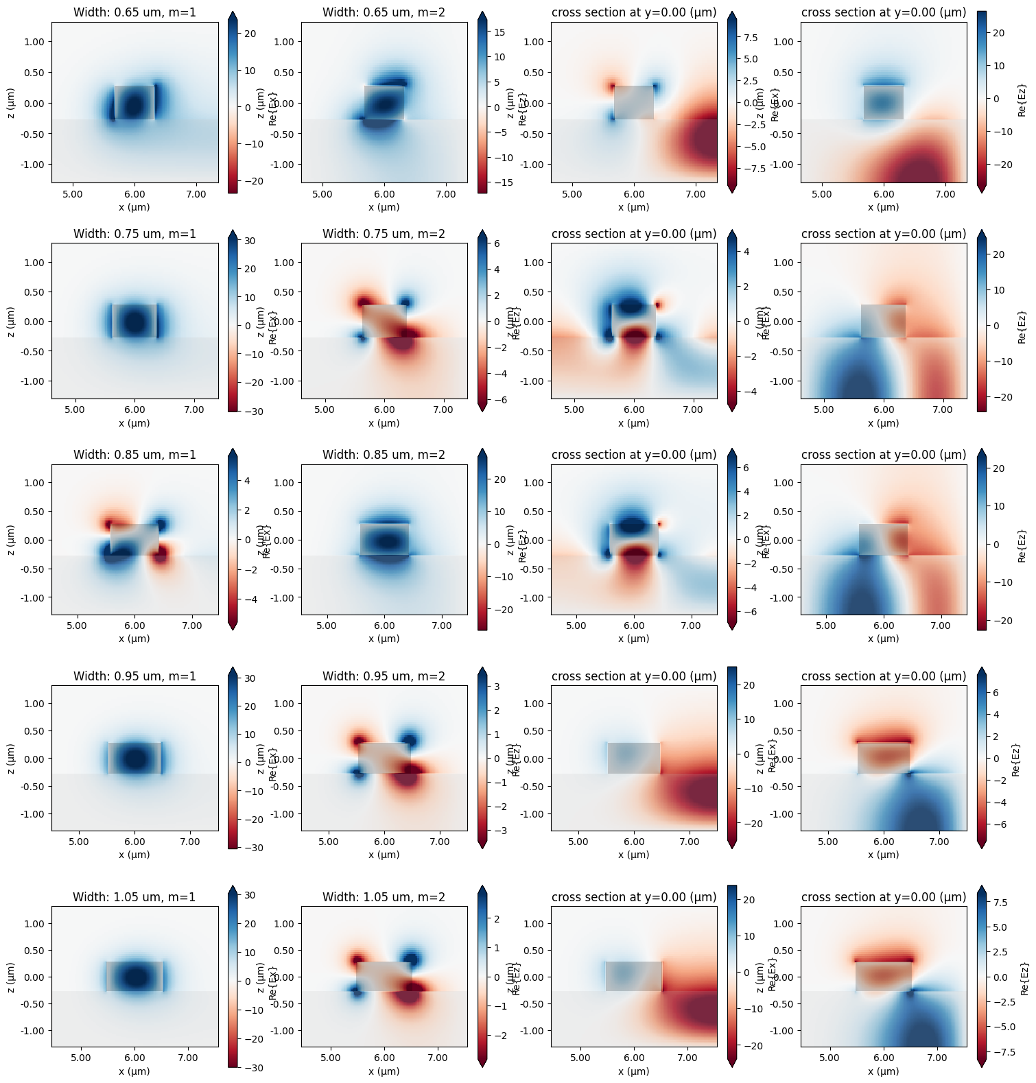
Define material models and geometric parameters. Diamond dispersion is fetched from refractiveindex.info and fitted to a pole-residue model via FastDispersionFitter. The mode sweep covers wavelengths 0.6–2.4 µm across five waveguide widths (0.65–1.05 µm).
def get_diamond_mat():
    url = "https://refractiveindex.info/data_csv.php?datafile=database/data/main/C/nk/Phillip.yml"
    # note that additional keyword arguments to load_nk_file get passed to np.loadtxt
    fitter = FastDispersionFitter.from_url(url)
    fitter = fitter.copy(update={"wvl_range": [0.4, 2.1]})
    advanced_param = AdvancedFastFitterParam(
        weights=(1, 1), num_iters=500, show_progress=True
    )
    diamond_mat, rms_error = fitter.fit(
        max_num_poles=3, advanced_param=advanced_param, tolerance_rms=0.01
    )
    return diamond_mat


def renamed_pole_residue(material, name):
    pole_args = {
        "name": name,
        "frequency_range": material.frequency_range,
        "allow_gain": material.allow_gain,
        "nonlinear_spec": material.nonlinear_spec,
        "modulation_spec": material.modulation_spec,
        "viz_spec": material.viz_spec,
        "heat_spec": material.heat_spec,
        "eps_inf": material.eps_inf,
        "poles": material.poles,
    }
    new_mat = td.PoleResidue(**pole_args)
    return new_mat


def renamed_medium(material, name):
    medium_args = {
        "name": name,
        "frequency_range": material.frequency_range,
        "allow_gain": material.allow_gain,
        "nonlinear_spec": material.nonlinear_spec,
        "modulation_spec": material.modulation_spec,
        "viz_spec": material.viz_spec,
        "heat_spec": material.heat_spec,
        "permittivity": material.permittivity,
        "conductivity": material.conductivity,
        "attrs": getattr(material, "attrs", None),
    }
    new_medium = td.Medium(**medium_args)
    return new_medium


mats = {
    "diamond": get_diamond_mat(),
    "nitride": td.material_library["Si3N4"]["Luke2015PMLStable"],
    "oxide": td.material_library["SiO2"]["Palik_Lossless"],
    "reflector": td.PECMedium(name="PEC"),
    "air": td.Medium(permittivity=1.0, name="air"),
}
material_names = ["diamond", "nitride", "oxide", "reflector", "air"]
material_ids = ["diamond", "nitride", "oxide", "PEC", "air"]


def rename_materials(mats_dict, mat_names, mat_ids):
    for m, m_id in zip(mat_names, mat_ids):
        if m_id == "PEC":
            mats_dict[m] = td.PECMedium(name=m)
        elif isinstance(mats_dict[m], td.Medium):
            mats_dict[m] = renamed_medium(mats_dict[m], m)
        else:
            mats_dict[m] = renamed_pole_residue(mats_dict[m], m)
    return mats_dict


rename_materials(mats, material_names, material_ids)
print(mats)
Output()
{'diamond': diamond, 'nitride': nitride, 'oxide': oxide, 'reflector': reflector, 'air': air}
idler_wavelength = 1.31
bend_radius = 6

######################################################### Mixer parameters #########################################################
layer_mats = ["diamond"]
n_idler = [mats[mat].nk_model(td.C_0 / idler_wavelength)[0] for mat in layer_mats]
layer_heights = [
    0.55
]  # [idler_wavelength/n_idler[i]/len(layer_mats) for i in range(len(layer_mats))]

min_width = 0.65
max_width = 1.05
num_widths = 5
swept_layer_widths = [
    np.linspace(min_width, max_width, num_widths) for _ in range(len(layer_mats))
]
wl_min = 0.6
wl_max = 2.4
f_min = td.C_0 / wl_max
f_max = td.C_0 / wl_min
num_freqs = 26
freqs = np.linspace(f_min, f_max, num_freqs)
freq_plot_i = np.argmin(np.abs(freqs - 146e12))

env = {}
mixer_env = {
    "layer_heights": np.array(layer_heights),
    "swept_layer_widths": np.array(swept_layer_widths),
    "chosen_layer_i": np.array(0),
    "num_modes": np.array(5),
    "freqs": np.array(freqs),
    "plotted_modes": np.array(2),
    "plot_fields": True,
    "plot_freq": freqs[freq_plot_i],
}
env["mixer"] = mixer_env

mode_env = {
    "layer_mats": layer_mats,
    "bend_radius": bend_radius,
    "cladding": "air",
    "box_mat": "oxide",
    "target_neff": None,
    "web_modes": False,
    "plot_geom": False,
    "material_library": mats,
    "return_fields": True,
}
env["mode"] = mode_env
######################################################### Nonlinear Bahar Parameters#########################################################
nonlinear_env = {
    #### Order of the signals is (signal, idler, pump A, pump B)
    "mode_nums": [0, 0, 0, 0],
    "mode_factors": [1, -1, 1, -1],
    "unit_ks": [1, 0, -1, 1],
}
env["nonlinear"] = nonlinear_env

net_momentum_env = {
    "fixed_freqs": td.C_0 / np.array([0.619, idler_wavelength]),
    "fit_tol": 1e-3,
    "poly_order": 15,
    "num_freqs": 1000,
}
env["net_momentum"] = net_momentum_env

fpm_env = {
    "zero_momentum_tolerance": 0.1,
    "pump_freq_nearby": None,
}
env["fpm"] = fpm_env

mn_env = {
    "mlim_a": (0, 50),
    "w_i": 1,
    "poly_order": 20,
}
env["mnumber"] = mn_env

result = {}
def build_layer_structures(
mats,
diamond_thickness,
box_thickness,
lower_nitride_thickness=0.22,
upper_nitride_thickness=0.0,
lower_nitride_top_depth=2.22,
upper_nitride_bottom_depth=2,
reflector_diamond_gap=0.87,
reflector_thickness=0.5,
ring_radius=6,
ring_width=0.85,
window_size=100,
add_lower_nitride=False,
):
"""Build all td.Structure objects for the diamond ring on nitride/oxide stack.
Returns:
structures: list of td.Structure
layer_z_centers: dict mapping layer name to z center coordinate
"""
# Compute z positions (same logic as original get_nitride_window_layer_stack)
zmin_lower_nitride = box_thickness
zmin_upper_nitride = (
zmin_lower_nitride
+ lower_nitride_thickness
+ lower_nitride_top_depth
- upper_nitride_bottom_depth
)
zmin_diamond = max(zmin_upper_nitride, zmin_upper_nitride + upper_nitride_thickness)
oxide_thickness = box_thickness + lower_nitride_thickness + lower_nitride_top_depth
structures = []
# 1. Oxide substrate (full slab)
structures.append(
td.Structure(
geometry=td.Box(
center=(0, 0, oxide_thickness / 2),
size=(td.inf, td.inf, oxide_thickness),
),
medium=mats["oxide"],
name="oxide",
)
)
# 2. Lower nitride film (structure only added if add_lower_nitride=True;
# lower_nitride_thickness still affects z positions of upper layers)
if lower_nitride_thickness > 0 and add_lower_nitride:
structures.append(
td.Structure(
geometry=td.Box(
center=(0, 0, zmin_lower_nitride + lower_nitride_thickness / 2),
size=(td.inf, td.inf, lower_nitride_thickness),
),
medium=mats["nitride"],
name="lower_nitride",
)
)
# 3. Upper nitride film (may be zero thickness)
if upper_nitride_thickness > 0:
structures.append(
td.Structure(
geometry=td.Box(
center=(0, 0, zmin_upper_nitride + upper_nitride_thickness / 2),
size=(td.inf, td.inf, upper_nitride_thickness),
),
medium=mats["nitride"],
name="upper_nitride",
)
)
# 4. Window (air etch region — centered rectangle)
half_w = window_size / 2
window_verts = [
(-half_w, -half_w),
(half_w, -half_w),
(half_w, half_w),
(-half_w, half_w),
]
structures.append(
td.Structure(
geometry=td.PolySlab(
vertices=window_verts,
axis=2,
slab_bounds=(
zmin_upper_nitride,
zmin_upper_nitride + upper_nitride_bottom_depth,
),
),
medium=td.Medium(), # air
name="window",
)
)
# 5. Reflector
if reflector_thickness > 0:
zmin_refl = zmin_diamond - reflector_diamond_gap - reflector_thickness
structures.append(
td.Structure(
geometry=td.Box(
center=(0, 0, zmin_refl + reflector_thickness / 2),
size=(td.inf, td.inf, reflector_thickness),
),
medium=mats["reflector"],
name="reflector",
)
)
# 6. Diamond ring — outer cylinder minus inner cylinder
z_center_diamond = zmin_diamond + diamond_thickness / 2
ring_geo = td.ClipOperation(
operation="difference",
geometry_a=td.Cylinder(
center=(0, 0, z_center_diamond),
radius=ring_radius + ring_width / 2,
length=diamond_thickness,
axis=2,
),
geometry_b=td.Cylinder(
center=(0, 0, z_center_diamond),
radius=ring_radius - ring_width / 2,
length=diamond_thickness,
axis=2,
),
)
structures.append(
td.Structure(geometry=ring_geo, medium=mats["diamond"], name="diamond_ring")
)
layer_z_centers = {
"diamond": z_center_diamond,
"lower_nitride": zmin_lower_nitride + lower_nitride_thickness / 2,
"upper_nitride": zmin_upper_nitride + upper_nitride_thickness / 2,
"oxide": oxide_thickness / 2,
}
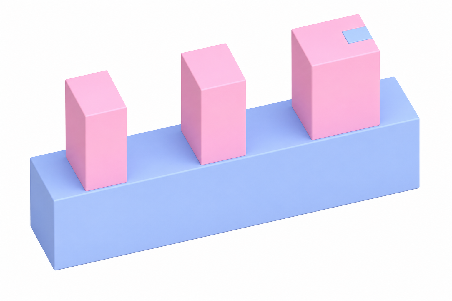
return structures, layer_z_centers
# Build the layer structures
layer_kwargs = {
"diamond_thickness": layer_heights[0],
"box_thickness": 10,
"upper_nitride_thickness": 0.0,
"lower_nitride_thickness": 0.22, # used for z-position calculation only; no structure added (add_lower_nitride=False)
"upper_nitride_bottom_depth": 2,
"lower_nitride_top_depth": 2.22,
"reflector_diamond_gap": 0.87,
"reflector_thickness": 0.5,
}
Effective Index Calculation
Sweep the diamond waveguide width and compute the effective refractive index of the fundamental TE-like mode over the full frequency range. Results are stored in a NeffMixer object that fits a polynomial dispersion model and predicts resonance frequencies for each mode number.
result["neff_mixer"] = get_neff_mixer(**env["mixer"], mode_args=env["mode"])
Plotting fields at 139.90 THz
  0%|          | 0/5 [00:00<?, ?it/s]/home/filipe/anaconda3/lib/python3.11/site-packages/scipy/sparse/_construct.py:543: FutureWarning: Input has data type int64, but the output has been cast to float64.  In the future, the output data type will match the input. To avoid this warning, set the `dtype` parameter to `None` to have the output dtype match the input, or set it to the desired output data type.
Note: In Python 3.11, this warning can be generated by a call of scipy.sparse.diags(), but the code indicated in the warning message will refer to an internal call of scipy.sparse.diags_array(). If that happens, check your code for the use of diags().
  A = diags_array(diagonals, offsets=offsets, shape=shape, dtype=dtype)
 20%|██        | 1/5 [01:48<07:12, 108.21s/it]/home/filipe/anaconda3/lib/python3.11/site-packages/scipy/sparse/_construct.py:543: FutureWarning: Input has data type int64, but the output has been cast to float64.  In the future, the output data type will match the input. To avoid this warning, set the `dtype` parameter to `None` to have the output dtype match the input, or set it to the desired output data type.
Note: In Python 3.11, this warning can be generated by a call of scipy.sparse.diags(), but the code indicated in the warning message will refer to an internal call of scipy.sparse.diags_array(). If that happens, check your code for the use of diags().
  A = diags_array(diagonals, offsets=offsets, shape=shape, dtype=dtype)
 40%|████      | 2/5 [02:23<03:15, 65.13s/it] /home/filipe/anaconda3/lib/python3.11/site-packages/scipy/sparse/_construct.py:543: FutureWarning: Input has data type int64, but the output has been cast to float64.  In the future, the output data type will match the input. To avoid this warning, set the `dtype` parameter to `None` to have the output dtype match the input, or set it to the desired output data type.
Note: In Python 3.11, this warning can be generated by a call of scipy.sparse.diags(), but the code indicated in the warning message will refer to an internal call of scipy.sparse.diags_array(). If that happens, check your code for the use of diags().
  A = diags_array(diagonals, offsets=offsets, shape=shape, dtype=dtype)
 60%|██████    | 3/5 [04:03<02:42, 81.17s/it]/home/filipe/anaconda3/lib/python3.11/site-packages/scipy/sparse/_construct.py:543: FutureWarning: Input has data type int64, but the output has been cast to float64.  In the future, the output data type will match the input. To avoid this warning, set the `dtype` parameter to `None` to have the output dtype match the input, or set it to the desired output data type.
Note: In Python 3.11, this warning can be generated by a call of scipy.sparse.diags(), but the code indicated in the warning message will refer to an internal call of scipy.sparse.diags_array(). If that happens, check your code for the use of diags().
  A = diags_array(diagonals, offsets=offsets, shape=shape, dtype=dtype)
 80%|████████  | 4/5 [05:14<01:17, 77.01s/it]/home/filipe/anaconda3/lib/python3.11/site-packages/scipy/sparse/_construct.py:543: FutureWarning: Input has data type int64, but the output has been cast to float64.  In the future, the output data type will match the input. To avoid this warning, set the `dtype` parameter to `None` to have the output dtype match the input, or set it to the desired output data type.
Note: In Python 3.11, this warning can be generated by a call of scipy.sparse.diags(), but the code indicated in the warning message will refer to an internal call of scipy.sparse.diags_array(). If that happens, check your code for the use of diags().
  A = diags_array(diagonals, offsets=offsets, shape=shape, dtype=dtype)
100%|██████████| 5/5 [06:28<00:00, 77.75s/it]
Phase Matching Via m-Number Selection
For each waveguide width, find the azimuthal mode-number quartet $(m_{\text{pump}_A},\,m_{\text{pump}_B},\,m_\text{signal},\,m_\text{idler})$ satisfying both energy and momentum conservation. fpm_spectrum scans allowed combinations using the polynomial dispersion fit and returns the phase-matched sets.
resonances_by_width = result["neff_mixer"].get_resonances(
    length=2 * np.pi * env["mode"]["bend_radius"] * 1e-6,
    plot=True,
    poly_order=env["mnumber"]["poly_order"],
)
m_pump_a, m_pump_b, f_as, f_bs, output_freqs = fpm_spectrum(
    resonances_by_width,
    env["nonlinear"],
    env["net_momentum"],
    w_i=env["mnumber"]["w_i"],
    plot=True,
    mlim_a=env["mnumber"]["mlim_a"],
)
output_fsr_freqs = np.abs(np.mean(np.diff(output_freqs)))
output_fsr_wavelengths = np.abs(np.mean(np.diff(c / output_freqs)))

result["output_fsr_freqs"] = output_fsr_freqs
result["output_fsr_wavelengths"] = output_fsr_wavelengths
result["m_pump_a"] = m_pump_a
result["m_pump_b"] = m_pump_b
result["f_as"] = f_as
result["f_bs"] = f_bs
result["output_freqs"] = output_freqs
result["resonances_by_width"] = resonances_by_width
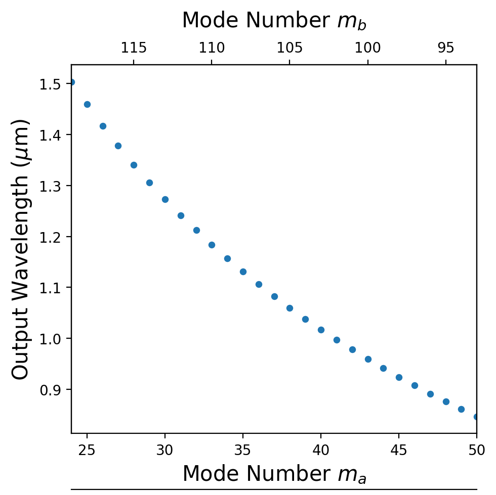
m_as = [26, 27, 28]
for m_a in m_as:
    m_i = np.argmin(np.abs(np.array(result["m_pump_a"]) - m_a))
    print(result["m_pump_a"][m_i])
    print(result["m_pump_b"][m_i])
    print(td.C_0 / result["f_as"][m_i])
    print(td.C_0 / result["f_bs"][m_i])
    print(td.C_0 / result["output_freqs"][m_i])
    print("--------------------------------")
26
117
2.281459598926598
0.7417002085006762
1.417291517955413
--------------------------------
27
116
2.2308186349488333
0.7473886499471527
1.3778225512388038
--------------------------------
28
115
2.1831044546995444
0.7531675928679139
1.340758578306063
--------------------------------
Resonance Locking
Run three FDTD simulations — one per resonance (signal, pump A, pump B) — using a ResonanceFinder monitor to precisely resolve each resonant frequency and quality factor. The locked frequencies are used in the nonlinear polarization computation.
# Ring and simulation parameters
ring_radius = env["mode"]["bend_radius"]
ring_width = env["mixer"]["swept_layer_widths"][0][env["mnumber"]["w_i"]]

# Build structures using cylinder-based ring
structures, layer_z_centers = build_layer_structures(
    mats=mats, ring_radius=ring_radius, ring_width=ring_width, **layer_kwargs
)

# Port at (0, -radius) pointing in +x direction (same as original orientation=0)
port_z_center = layer_z_centers["diamond"]
port_size_mult = (4, 2.5)
port_info = {
    "o1": {
        "center": (0, -ring_radius, port_z_center),
        "size": (0, ring_width * port_size_mult[0], ring_width * port_size_mult[1]),
        "direction": "-",
        "mode_spec": td.ModeSpec(
            num_modes=10,
            filter_pol="te",
            bend_radius=-ring_radius,
            bend_axis=1,
            num_pml=(5, 5),
        ),
    }
}

# Frequency range for modeler (used for default bandwidth calculations)
modeler_bandwidth = 0.02  # um
modeler_num_freqs = 3
modeler_wavelength = 1.55  # original get_component_modeler default
# Fixed modeler freqs (original always used wavelength=1.55)
modeler_freqs = td.C_0 / np.linspace(
    modeler_wavelength - modeler_bandwidth / 2,
    modeler_wavelength + modeler_bandwidth / 2,
    modeler_num_freqs,
)

# Base simulation
base_sim = td.Simulation(
    size=(2 * ring_radius + 4, 2 * ring_radius + 4, 4),
    center=(0, 0, port_z_center),
    structures=structures,
    grid_spec=td.GridSpec.auto(wavelength=idler_wavelength, min_steps_per_wvl=20),
    boundary_spec=td.BoundarySpec(
        x=td.Boundary(minus=td.PML(), plus=td.PML()),
        y=td.Boundary(minus=td.PML(), plus=td.PML()),
        z=td.Boundary(minus=td.PML(), plus=td.PML()),
    ),
    run_time=2e-12,
    symmetry=(0, 0, 0),
)

env["port_info"] = port_info
env["layer_z_centers"] = layer_z_centers
env["base_sim"] = base_sim
env["modeler_freqs"] = modeler_freqs

env["custom_fdtd"] = {}
env["chi3_reslock"] = {
    "downsample": (2, 2, 2),
    "mode_volume_layer": "diamond",
    "ff_res": 60,
    "amp_a": 1000,
    "amp_b": 1000,
    "Q_threshold": 1e3,
}
freq_i = np.argmin(
    np.abs(result["output_freqs"] - env["net_momentum"]["fixed_freqs"][1])
)
f_a = result["f_as"][freq_i]
f_b = result["f_bs"][freq_i]
f_sig = env["net_momentum"]["fixed_freqs"][0]
f_idl = result["output_freqs"][freq_i]

wavelengths = {
    "pump_A": td.C_0 / f_a,
    "pump_B": td.C_0 / f_b,
    "signal": td.C_0 / f_sig,
    "idler": td.C_0 / f_idl,
}

sim_names = ["signal", "pump_A", "pump_B"]
resolutions = [20, 20, 20]
run_times = [2e-12, 2e-12, 2e-12]
freqs = [f_sig, f_a, f_b]
result["chi3_reslock"] = {}
for sim_name, res, run_time, freq in zip(sim_names, resolutions, run_times, freqs):
    inputs = {
        "o1": {
            "modes": [0],
            "amps": [1],
            "phases": [0],
            "freqs": [freq],
            "fwidths": [None],
        },
    }
    outputs = {"o1": {"types": ["time_Ey"]}}
    mode_volume = {
        "layer": env["chi3_reslock"]["mode_volume_layer"],
        "thickness": np.sum(env["mixer"]["layer_heights"]) + 0.1,
        "downsample": env["chi3_reslock"]["downsample"],
        "apodization": {"start": 1e-12, "width": run_time / 10},
    }
    output_freqs = [freq]
    sim_kwargs = {"normalize_index": None, "size": [16, 16, 4]}

    # Update base simulation with current run_time and resolution
    current_sim = env["base_sim"].updated_copy(
        run_time=run_time,
        grid_spec=td.GridSpec.auto(wavelength=1.55, min_steps_per_wvl=res),
    )

    # Build and run the simulation
    sim = get_fdtd_sim(
        simulation=current_sim,
        ports=env["port_info"],
        freqs=env["modeler_freqs"],
        layer_z_centers=env["layer_z_centers"],
        inputs=inputs,
        outputs=outputs,
        mode_volume=mode_volume,
        output_freqs=output_freqs,
        sim_kwargs=sim_kwargs,
    )
    sim_job = td.web.Job(simulation=sim, task_name=f"{sim_name}_chi3_reslock")
    sim_data = sim_job.run()

    # Find the closest resonance above the Q threshold
    bandwidth = 0.02  # um, matches original modeler bandwidth
    wl_min = wavelengths[sim_name] - bandwidth / 2
    wl_max = wavelengths[sim_name] + bandwidth / 2
    fmin, fmax = td.C_0 / wl_max, td.C_0 / wl_min
    resonance_finder = ResonanceFinder(freq_window=(fmin, fmax))
    resonance_data = resonance_finder.run(signals=sim_data.monitor_data["o1_time_Ey"])
    df = resonance_data.to_dataframe()
    result["chi3_reslock"][sim_name] = {}
    df_valid = df[np.abs(df["Q"]) > env["chi3_reslock"]["Q_threshold"]]
    result["chi3_reslock"][sim_name]["Q_df"] = df
    result["chi3_reslock"][sim_name]["Q_df_valid"] = df_valid

    idx = np.argmin(np.abs(df_valid.index.to_numpy() - td.C_0 / wavelengths[sim_name]))
    closest_res_f = df_valid.index[idx]
    result["chi3_reslock"][sim_name]["resonance_freq"] = closest_res_f
    result["chi3_reslock"][sim_name]["resonance_freq_idx"] = idx
16:04:55 -03 Created task 'signal_chi3_reslock' with resource_id
             'fdve-805154d6-9101-4a4b-80a3-8c8d0797cce7' and task_type 'FDTD'.
             View task using web UI at
             'https://tidy3d.simulation.cloud/workbench?taskId=fdve-805154d6-910
             1-4a4b-80a3-8c8d0797cce7'.
Task folder: 'default'.
Output()
16:05:00 -03 Estimated FlexCredit cost: 0.809. Minimum cost depends on task
             execution details. Use 'web.real_cost(task_id)' to get the billed
             FlexCredit cost after a simulation run.
16:05:02 -03 status = success
Output()
16:05:22 -03 Loading simulation from simulation_data.hdf5
16:05:23 -03 Created task 'pump_A_chi3_reslock' with resource_id
             'fdve-e52a26dd-e220-4e52-bc59-1031a60bc3f4' and task_type 'FDTD'.
             View task using web UI at
             'https://tidy3d.simulation.cloud/workbench?taskId=fdve-e52a26dd-e22
             0-4e52-bc59-1031a60bc3f4'.
Task folder: 'default'.
Output()
16:05:28 -03 Estimated FlexCredit cost: 0.808. Minimum cost depends on task
             execution details. Use 'web.real_cost(task_id)' to get the billed
             FlexCredit cost after a simulation run.
16:05:30 -03 status = success
Output()
16:05:40 -03 Loading simulation from simulation_data.hdf5
16:05:43 -03 Created task 'pump_B_chi3_reslock' with resource_id
             'fdve-f6555b58-56d8-4770-910a-bf856a96c898' and task_type 'FDTD'.
             View task using web UI at
             'https://tidy3d.simulation.cloud/workbench?taskId=fdve-f6555b58-56d
             8-4770-910a-bf856a96c898'.
Task folder: 'default'.
Output()
16:05:49 -03 Estimated FlexCredit cost: 0.809. Minimum cost depends on task
             execution details. Use 'web.real_cost(task_id)' to get the billed
             FlexCredit cost after a simulation run.
16:05:51 -03 status = success
Output()
16:06:22 -03 Loading simulation from simulation_data.hdf5
print(result["chi3_reslock"]["signal"])
print(result["chi3_reslock"]["pump_A"])
print(result["chi3_reslock"]["pump_B"])
{'Q_df':                      decay            Q  amplitude     phase     error
freq
4.724864e+14  2.988213e+11  4967.383062   0.438663 -2.860279  0.000526
4.753390e+14  1.552170e+11  9620.863825   0.362880  2.888826  0.000341
4.782399e+14  2.084022e+11  7209.304841   0.395091  2.461943  0.000404
4.811215e+14  5.157990e+11  2930.380995   0.586883  1.957723  0.000457
4.868306e+14  3.706404e+11  4126.435320   0.449405  1.148452  0.000290
4.896939e+14  3.835812e+11  4010.672963   0.463494  0.673537  0.000128
4.925552e+14  4.264920e+11  3628.222457   0.465331  0.176524  0.000399
4.953925e+14  3.024737e+11  5145.311674   0.415709 -0.307896  0.000689
5.002050e+14  2.260458e+13    69.518671   0.780105 -1.774624  0.010654, 'Q_df_valid':                      decay            Q  amplitude     phase     error
freq
4.724864e+14  2.988213e+11  4967.383062   0.438663 -2.860279  0.000526
4.753390e+14  1.552170e+11  9620.863825   0.362880  2.888826  0.000341
4.782399e+14  2.084022e+11  7209.304841   0.395091  2.461943  0.000404
4.811215e+14  5.157990e+11  2930.380995   0.586883  1.957723  0.000457
4.868306e+14  3.706404e+11  4126.435320   0.449405  1.148452  0.000290
4.896939e+14  3.835812e+11  4010.672963   0.463494  0.673537  0.000128
4.925552e+14  4.264920e+11  3628.222457   0.465331  0.176524  0.000399
4.953925e+14  3.024737e+11  5145.311674   0.415709 -0.307896  0.000689, 'resonance_freq': np.float64(486830627499313.7), 'resonance_freq_idx': np.int64(4)}
{'Q_df':                      decay            Q  amplitude     phase     error
freq
1.373074e+14 -1.622774e+11 -2658.187524   0.951105  3.072118  0.000689
1.401997e+14 -2.225918e+11 -1978.735116   1.083997  1.563692  0.000595
1.430847e+14 -2.923336e+11 -1537.674154   1.013239  0.063220  0.000598
1.515495e+14 -2.092342e+12  -227.547209   2.286071  1.979913  0.001269, 'Q_df_valid':                      decay            Q  amplitude     phase     error
freq
1.373074e+14 -1.622774e+11 -2658.187524   0.951105  3.072118  0.000689
1.401997e+14 -2.225918e+11 -1978.735116   1.083997  1.563692  0.000595
1.430847e+14 -2.923336e+11 -1537.674154   1.013239  0.063220  0.000598, 'resonance_freq': np.float64(140199681691107.67), 'resonance_freq_idx': np.int64(1)}
{'Q_df':                      decay            Q  amplitude     phase     error
freq
3.700458e+14  3.295505e+13    35.276337   7.321571  0.140748  0.087510
3.790765e+14  1.119937e+13   106.336721   0.170488 -2.433405  0.038314
3.875827e+14  6.054486e+11  2011.115405   0.720514  3.076572  0.001276
3.905454e+14  3.661043e+11  3351.325179   0.540876  2.321923  0.001307
3.934941e+14  2.581874e+11  4787.987931   0.531242  1.712725  0.001962
3.964756e+14  2.869032e+11  4341.410886   0.575101  1.151010  0.001999
3.994449e+14  3.104318e+11  4042.412211   0.621082  0.663967  0.001929
4.024362e+14  4.419741e+11  2860.553233   0.795676  0.235923  0.001179
4.041121e+14 -1.533599e+13   -82.782737   2.141887 -0.282314  0.007875, 'Q_df_valid':                      decay            Q  amplitude     phase     error
freq
3.875827e+14  6.054486e+11  2011.115405   0.720514  3.076572  0.001276
3.905454e+14  3.661043e+11  3351.325179   0.540876  2.321923  0.001307
3.934941e+14  2.581874e+11  4787.987931   0.531242  1.712725  0.001962
3.964756e+14  2.869032e+11  4341.410886   0.575101  1.151010  0.001999
3.994449e+14  3.104318e+11  4042.412211   0.621082  0.663967  0.001929
4.024362e+14  4.419741e+11  2860.553233   0.795676  0.235923  0.001179, 'resonance_freq': np.float64(393494132733729.2), 'resonance_freq_idx': np.int64(2)}
χ³ Polarization Generation
Interpolate the three locked field profiles onto a common spatial grid. The $\chi^{(3)}$ polarization driving the idler is:
$$\mathbf{P}^{(3)} \propto \chi^{(3)}\, \mathbf{E}_{\text{pump}_A}\, \mathbf{E}_{\text{pump}_B}\, \mathbf{E}^*_\text{signal}$$
chi3_pol_env = {
    "downsample": (1, 1, 1),
    "mode_volume_layer": "diamond",
    "ff_res": 60,
    "amp_a": 1000,
    "amp_b": 1000,
    "Q_threshold": 1e4,
    "resonance_idx_offset": [0, 1, 2],
    "sim_names": ["signal", "pump_A", "pump_B"],
    "sim_nl_index": [0, 2, 3],
    "run_time": 2e-12,
    "sim_res": 20,
    "freq_res": 5,
    "freq_bw": 2e12,
    "freq_idxs": [2, 2, 2],
}
env["chi3_polarization"] = chi3_pol_env

sim_names = env["chi3_polarization"]["sim_names"]
freqs = []
for sim_i, sim_name in enumerate(sim_names):
    resonance_idx = (
        result["chi3_reslock"][sim_name]["resonance_freq_idx"]
        + env["chi3_polarization"]["resonance_idx_offset"][sim_i]
    )
    freqs.append(result["chi3_reslock"][sim_name]["Q_df_valid"].index[resonance_idx])

for sim_i, (sim_name, freq) in enumerate(zip(sim_names, freqs)):
    inputs = {
        "o1": {
            "modes": [0],
            "amps": [1],
            "phases": [0],
            "freqs": [freq],
            "fwidths": [None],
        },
    }
    outputs = {"o1": {"types": ["time_Ey"]}}
    mode_volume = {
        "layer": env["chi3_polarization"]["mode_volume_layer"],
        "colocate": False,
        "thickness": np.sum(env["mixer"]["layer_heights"]) + 0.1,
        "downsample": env["chi3_polarization"]["downsample"],
        "apodization": {
            "start": env["chi3_polarization"]["run_time"] / 3,
            "width": env["chi3_polarization"]["run_time"] / 10,
        },
    }
    if env["chi3_polarization"]["freq_res"] == 1:
        output_freqs = [freq]
    else:
        output_freqs = np.linspace(
            freq - env["chi3_polarization"]["freq_bw"] / 2,
            freq + env["chi3_polarization"]["freq_bw"] / 2,
            env["chi3_polarization"]["freq_res"],
        )
    sim_kwargs = {"normalize_index": None, "size": [16, 16, 4]}

    # Update base simulation
    current_sim = env["base_sim"].updated_copy(
        run_time=env["chi3_polarization"]["run_time"],
        grid_spec=td.GridSpec.auto(
            wavelength=1.55, min_steps_per_wvl=env["chi3_polarization"]["sim_res"]
        ),
    )

    # Build and run the simulation
    sim = get_fdtd_sim(
        simulation=current_sim,
        ports=env["port_info"],
        freqs=env["modeler_freqs"],
        layer_z_centers=env["layer_z_centers"],
        inputs=inputs,
        outputs=outputs,
        mode_volume=mode_volume,
        output_freqs=output_freqs,
        sim_kwargs=sim_kwargs,
    )
    sim_job = td.web.Job(simulation=sim, task_name=f"{sim_name}_chi3_polarization")
    sim_data = sim_job.run()
    result[sim_name] = sim_data
    sim_nl_index = env["chi3_polarization"]["sim_nl_index"]
    if sim_i == 0:
        # Get the minimum and maximum x, y, and z values for all the fields
        min_x = np.min(sim_data["field"].Ex.y.values)
        max_x = np.max(sim_data["field"].Ex.y.values)
        res_x = np.max([len(sim_data["field"].Ex.x.values) for sim_name in sim_names])
        min_y = np.min(sim_data["field"].Ex.y.values)
        max_y = np.max(sim_data["field"].Ex.y.values)
        res_y = np.max([len(sim_data["field"].Ex.y.values) for sim_name in sim_names])
        min_z = np.min(sim_data["field"].Ex.z.values)
        max_z = np.max(sim_data["field"].Ex.z.values)
        res_z = np.max([len(sim_data["field"].Ex.z.values) for sim_name in sim_names])
        x_interp = np.linspace(min_x, max_x, res_x)
        y_interp = np.linspace(min_y, max_y, res_y)
        z_interp = np.linspace(min_z, max_z, res_z)
16:06:23 -03 Created task 'signal_chi3_polarization' with resource_id
             'fdve-4c07409d-76dd-4dbc-a5e0-88253c50288e' and task_type 'FDTD'.
             View task using web UI at
             'https://tidy3d.simulation.cloud/workbench?taskId=fdve-4c07409d-76d
             d-4dbc-a5e0-88253c50288e'.
Task folder: 'default'.
Output()
16:06:28 -03 Estimated FlexCredit cost: 0.844. Minimum cost depends on task
             execution details. Use 'web.real_cost(task_id)' to get the billed
             FlexCredit cost after a simulation run.
16:06:31 -03 status = success
Output()
16:07:40 -03 Loading simulation from simulation_data.hdf5
16:07:49 -03 Created task 'pump_A_chi3_polarization' with resource_id
             'fdve-d6bf5fa3-3467-44d2-ab6e-32997f1d2ac8' and task_type 'FDTD'.
             View task using web UI at
             'https://tidy3d.simulation.cloud/workbench?taskId=fdve-d6bf5fa3-346
             7-44d2-ab6e-32997f1d2ac8'.
Task folder: 'default'.
Output()
16:07:54 -03 Estimated FlexCredit cost: 0.818. Minimum cost depends on task
             execution details. Use 'web.real_cost(task_id)' to get the billed
             FlexCredit cost after a simulation run.
16:07:56 -03 status = success
Output()
16:09:05 -03 Loading simulation from simulation_data.hdf5
16:09:09 -03 Created task 'pump_B_chi3_polarization' with resource_id
             'fdve-ce8dc2e1-480d-4570-8e55-5a679e0ef33e' and task_type 'FDTD'.
             View task using web UI at
             'https://tidy3d.simulation.cloud/workbench?taskId=fdve-ce8dc2e1-480
             d-4570-8e55-5a679e0ef33e'.
Task folder: 'default'.
Output()
16:09:14 -03 Estimated FlexCredit cost: 0.837. Minimum cost depends on task
             execution details. Use 'web.real_cost(task_id)' to get the billed
             FlexCredit cost after a simulation run.
16:09:16 -03 status = success
Output()
16:10:20 -03 Loading simulation from simulation_data.hdf5
efield_list = []
method = "linear"
# Interpolate the fields onto the same spatial grid
for i, sim_name in enumerate(sim_names):
    freq_idx = env["chi3_polarization"]["freq_idxs"][i]
    original_field = result[sim_name]["field"]
    dataset_E = td.FieldDataset(
        Ex=td.ScalarFieldDataArray(
            original_field.Ex.isel(f=freq_idx).interp(
                x=x_interp,
                y=y_interp,
                z=z_interp,
                method=method,
                assume_sorted=True,
                kwargs={"fill_value": 0},
            )
        ).expand_dims(f=[original_field.Ex.f.values[freq_idx]]),
        Ey=td.ScalarFieldDataArray(
            original_field.Ey.isel(f=freq_idx).interp(
                x=x_interp,
                y=y_interp,
                z=z_interp,
                method=method,
                assume_sorted=True,
                kwargs={"fill_value": 0},
            )
        ).expand_dims(f=[original_field.Ey.f.values[freq_idx]]),
        Ez=td.ScalarFieldDataArray(
            original_field.Ez.isel(f=freq_idx).interp(
                x=x_interp,
                y=y_interp,
                z=z_interp,
                method=method,
                assume_sorted=True,
                kwargs={"fill_value": 0},
            )
        ).expand_dims(f=[original_field.Ez.f.values[freq_idx]]),
    )
    efield_list.append(dataset_E)

# Get the n2
coords = td.Coords(x=x_interp, y=y_interp, z=z_interp)
n2 = n2_on_coords(sim=result[sim_names[0]].simulation, coords=coords)


# Combine the fields into a single FieldDataset with nonlinearly conjugated fields
def if_conj(E, should_conj):
    return E.conj() if should_conj == -1 else E


combined_Ex = xr.concat(
    [
        if_conj(
            E.Ex, env["nonlinear"]["mode_factors"][i] * env["nonlinear"]["unit_ks"][i]
        )
        for E, i in zip(efield_list, sim_nl_index)
    ],
    dim="f",
)
combined_Ey = xr.concat(
    [
        if_conj(
            E.Ey, env["nonlinear"]["mode_factors"][i] * env["nonlinear"]["unit_ks"][i]
        )
        for E, i in zip(efield_list, sim_nl_index)
    ],
    dim="f",
)
combined_Ez = xr.concat(
    [
        if_conj(
            E.Ez, env["nonlinear"]["mode_factors"][i] * env["nonlinear"]["unit_ks"][i]
        )
        for E, i in zip(efield_list, sim_nl_index)
    ],
    dim="f",
)
combined_E = td.FieldDataset(Ex=combined_Ex, Ey=combined_Ey, Ez=combined_Ez)
freqs = combined_Ex.f.values
output_freq = [
    np.sum(
        [f * env["nonlinear"]["mode_factors"][i] for f, i in zip(freqs, sim_nl_index)]
    )
]
p_Ex = combined_Ex.prod(dim="f").expand_dims(f=output_freq)
p_Ey = combined_Ey.prod(dim="f").expand_dims(f=output_freq)
p_Ez = combined_Ez.prod(dim="f").expand_dims(f=output_freq)

polarization = td.FieldDataset(Ex=p_Ex, Ey=p_Ey, Ez=p_Ez)

result["efield"] = combined_E
result["n2"] = n2
result["polarization"] = polarization

# Create 2D meshgrid of x and y coordinates
X, Y = np.meshgrid(
    result["polarization"].Ex.x, result["polarization"].Ex.y, indexing="ij"
)  # Shape: (x, y)
# Compute theta (angle in the x–y plane) at each (x, y) position
theta = np.arctan2(Y, X)  # Shape: (x, y), handles all quadrants
# Convert theta into an xarray.DataArray with matching coords
theta_da = xr.DataArray(
    theta,
    coords={"x": result["polarization"].Ex.x, "y": result["polarization"].Ex.y},
    dims=("x", "y"),
)
# Expand theta to match shape of Ex and Ey (broadcast over z)
theta_expanded = theta_da.expand_dims(z=result["polarization"].Ex.z)  # dims: (x, y, z)
# Now compute Er
polarization_Er = result["polarization"].Ex * np.cos(theta_expanded) + result[
    "polarization"
].Ey * np.sin(theta_expanded)
combined_Er = combined_E.Ex * np.cos(theta_expanded) + combined_E.Ey * np.sin(
    theta_expanded
)
result["polarization_Er"] = polarization_Er
result["combined_Er"] = combined_Er


fig, ax = plt.subplots(2, max(len(result["efield"].Ex.f), 3), figsize=(10, 10), dpi=400)
z_i = len(result["combined_Er"].z) // 2
for i in range(len(result["combined_Er"].f)):
    ax[0, i].set_aspect("equal")
    ax[1, i].set_aspect("equal")
    result["combined_Er"].isel(f=i, z=z_i).real.plot(
        x="x", y="y", ax=ax[0, i], add_colorbar=False
    )
    ax[0, i].set_title(
        r"Re{E$_{r}$}"
        + f" at {td.C_0 / result['combined_Er'].f.values[i] * 1e3:.2f} nm"
    )
    ax[0, i].set_xlabel("x ($\\mu$m)")
    ax[0, i].set_ylabel("y ($\\mu$m)")
    ax[0, i].set_xticks([-6, 0, 6])
    ax[0, i].set_yticks([-6, 0, 6])
    ax[0, i].tick_params(labelsize=13)

im = (
    (result["polarization_Er"].abs / result["polarization_Er"].abs.max())
    .isel(f=0, z=z_i)
    .plot(x="x", y="y", ax=ax[1, 0], add_colorbar=False)
)
cbar = fig.colorbar(im, ax=ax[1, 0], shrink=0.38)  # shrink to 60% of normal size
cbar.set_ticks([0, 0.5, 1])
cbar.ax.tick_params(labelsize=13)
cbar.set_ticklabels([r"$0$", r"$|P_r|$", r"$1$"])

ax[1, 0].set_title("")  # at {td.C_0/result["polarization"].Ex.f.values[0]*1e3:.2f} nm')
ax[1, 0].set_xlabel("x ($\\mu$m)")
ax[1, 0].set_ylabel("y ($\\mu$m)")
ax[1, 0].set_xticks([-6, 0, 6])
ax[1, 0].tick_params(labelsize=13)
ax[1, 0].set_yticks([-6, 0, 6])

im = xr.ufuncs.angle(
    xr.where(
        result["n2"].isel(z=z_i) > 0, result["polarization_Er"].isel(f=0, z=z_i), np.nan
    )
).plot(x="x", y="y", ax=ax[1, 1], add_colorbar=False)
im.set_clim(-np.pi, np.pi)
cbar = fig.colorbar(im, ax=ax[1, 1], shrink=0.38)  # shrink to 60% of normal size

cbar.set_ticks([-np.pi, 0, np.pi])
cbar.ax.tick_params(labelsize=13)
cbar.set_ticklabels([r"$-\pi$", r"$\angle P_r$", r"$\pi$"])
ax[1, 1].set_title("")
ax[1, 1].set_xlabel("x ($\\mu$m)")
ax[1, 1].tick_params(labelsize=13)
ax[1, 1].set_ylabel("y ($\\mu$m)")
ax[1, 1].set_xticks([-6, 0, 6])
ax[1, 1].set_yticks([-6, 0, 6])

im = result["n2"].isel(z=z_i).plot(x="x", y="y", ax=ax[1, 2], add_colorbar=False)
cbar = fig.colorbar(im, ax=ax[1, 2], shrink=0.38)  # shrink to 60% of normal size
ax[1, 2].set_title("n2")
ax[1, 2].set_xlabel("x ($\\mu$m)")
ax[1, 2].set_ylabel("y ($\\mu$m)")
plt.tight_layout()
plt.show()
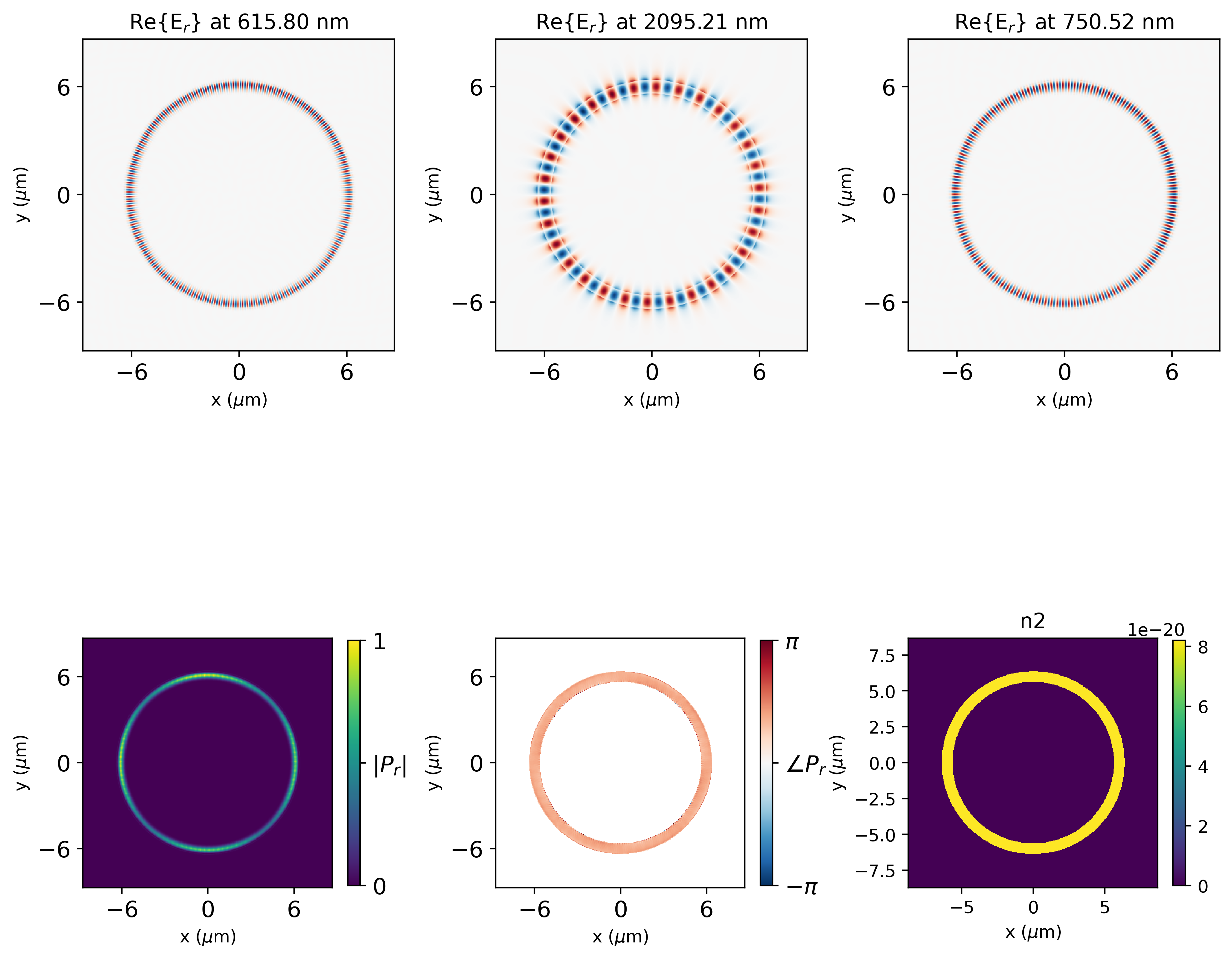
Output Mode Quality Factor and Mode Volume
Inject the nonlinear polarization as a CustomCurrentSource into the ring. Far-field monitors record the idler emission pattern in the upper hemisphere; flux monitors measure total radiated power. The quality factor $Q$ and mode volume $V$ quantify the FWM conversion efficiency.
def overlap_coeff(E1, E2, scale=1e30, mask=1):
    E1 = td.FieldDataset(
        Ex=E1.Ex * scale * mask, Ey=E1.Ey * scale * mask, Ez=E1.Ez * scale * mask
    )
    E2 = td.FieldDataset(
        Ex=E2.Ex * scale * mask, Ey=E2.Ey * scale * mask, Ez=E2.Ez * scale * mask
    )
    numerator = E1.Ex.conj() * E2.Ex + E1.Ey.conj() * E2.Ey + E1.Ez.conj() * E2.Ez
    numerator.real.isel(z=0, f=0).plot(x="x", y="y")
    numerator = numerator.integrate("x").integrate("y").integrate("z").values
    d_E1 = E1.Ex.abs**2 + E1.Ey.abs**2 + E1.Ez.abs**2
    d_E2 = E2.Ex.abs**2 + E2.Ey.abs**2 + E2.Ez.abs**2
    denominator = np.sqrt(
        d_E1.integrate("x").integrate("y").integrate("z").values
        * d_E2.integrate("x").integrate("y").integrate("z").values
    )
    return numerator / denominator
chi3_qv_env = {
    "downsample": (1, 1, 1),
    "ff_res": 600,
    "run_time": 1.8e-12,
    "sim_res": 20,
    "amps": 1e30,
}
env["chi3_qv"] = chi3_qv_env

inputs = {}
outputs = {}
mode_volume = {
    "layer": env["chi3_polarization"]["mode_volume_layer"],
    "thickness": np.sum(env["mixer"]["layer_heights"]) + 0.1,
    "downsample": env["chi3_qv"]["downsample"],
}
farfield = {
    "downsample": env["chi3_qv"]["downsample"],
    "surface": "spherical",
    "res": env["chi3_qv"]["ff_res"],
    "exclude_surfaces": ("x-", "x+", "y-", "y+", "z-"),
}
flux = {
    "downsample": env["chi3_qv"]["downsample"],
}
freq = result["polarization"].Ex.f.values[0]
pulse = td.GaussianPulse(freq0=freq, fwidth=freq / 10)
polarization = result["polarization"]
x, y, z = polarization.Ex.x.values, polarization.Ex.y.values, polarization.Ex.z.values
z_center = np.mean(z)
polarization = td.FieldDataset(
    Ex=polarization.Ex.assign_coords(z=z - z_center) * env["chi3_qv"]["amps"],
    Ey=polarization.Ey.assign_coords(z=z - z_center) * env["chi3_qv"]["amps"],
    Ez=polarization.Ez.assign_coords(z=z - z_center) * env["chi3_qv"]["amps"],
)
size = (np.max(x) - np.min(x), np.max(y) - np.min(y), np.max(z) - np.min(z))
custom_sources = [
    td.CustomCurrentSource(
        center=(0, 0, z_center),
        size=size,
        current_dataset=polarization,
        source_time=pulse,
    )
]
output_freqs = [freq]
sim_kwargs = {"normalize_index": None, "size": [35, 35, 6]}

# Update base simulation for QV
current_sim = env["base_sim"].updated_copy(
    run_time=env["chi3_qv"]["run_time"],
    grid_spec=td.GridSpec.auto(
        wavelength=1.55, min_steps_per_wvl=env["chi3_qv"]["sim_res"]
    ),
)

# Port info for QV: original used port_size_mult=(6,3) and no num_pml
ring_width_qv = env["mixer"]["swept_layer_widths"][0][env["mnumber"]["w_i"]]
qv_port_info = {
    "o1": {
        "center": env["port_info"]["o1"]["center"],
        "size": (0, ring_width_qv * 6, ring_width_qv * 3),
        "direction": env["port_info"]["o1"]["direction"],
        "mode_spec": td.ModeSpec(
            num_modes=10,
            filter_pol="te",
            bend_radius=-env["mode"]["bend_radius"],
            bend_axis=1,
        ),
    }
}


x_interp = result["polarization"].Ex.x.values
y_interp = result["polarization"].Ex.y.values
z_interp = result["polarization"].Ex.z.values

# Build and run the simulation
sim = get_fdtd_sim(
    simulation=current_sim,
    ports=qv_port_info,
    freqs=env["modeler_freqs"],
    layer_z_centers=env["layer_z_centers"],
    inputs=inputs,
    outputs=outputs,
    mode_volume=mode_volume,
    farfield=farfield,
    flux=flux,
    output_freqs=output_freqs,
    custom_sources=custom_sources,
    sim_kwargs=sim_kwargs,
)
sim_job = td.web.Job(simulation=sim, task_name=f"{sim_name}_chi3_qv")
sim_data = sim_job.run()

original_field = sim_data["field"]
coords = {
    "x": x_interp,
    "y": y_interp,
    "z": z_interp,
    "f": original_field.Ex.f.values,
}
method = "linear"
field_interp = td.FieldDataset(
    Ex=td.ScalarFieldDataArray(
        original_field.Ex.interp(
            x=x_interp, y=y_interp, z=z_interp, method=method, assume_sorted=True
        )
        .fillna(0)
        .values,
        coords=coords,
    ),
    Ey=td.ScalarFieldDataArray(
        original_field.Ey.interp(
            x=x_interp, y=y_interp, z=z_interp, method=method, assume_sorted=True
        )
        .fillna(0)
        .values,
        coords=coords,
    ),
    Ez=td.ScalarFieldDataArray(
        original_field.Ez.interp(
            x=x_interp, y=y_interp, z=z_interp, method=method, assume_sorted=True
        )
        .fillna(0)
        .values,
        coords=coords,
    ),
    Hx=td.ScalarFieldDataArray(
        original_field.Hx.interp(
            x=x_interp, y=y_interp, z=z_interp, method=method, assume_sorted=True
        )
        .fillna(0)
        .values,
        coords=coords,
    ),
    Hy=td.ScalarFieldDataArray(
        original_field.Hy.interp(
            x=x_interp, y=y_interp, z=z_interp, method=method, assume_sorted=True
        )
        .fillna(0)
        .values,
        coords=coords,
    ),
    Hz=td.ScalarFieldDataArray(
        original_field.Hz.interp(
            x=x_interp, y=y_interp, z=z_interp, method=method, assume_sorted=True
        )
        .fillna(0)
        .values,
        coords=coords,
    ),
)
E_2 = field_interp.Ex.abs**2 + field_interp.Ey.abs**2 + field_interp.Ez.abs**2
H_2 = field_interp.Hx.abs**2 + field_interp.Hy.abs**2 + field_interp.Hz.abs**2


n = mats[env["chi3_polarization"]["mode_volume_layer"]].nk_model(
    td.C_0 / idler_wavelength
)[0]
nonlinear_mask = xr.where(result["n2"] > 0, 1, 0)
eps = n**2 * td.EPSILON_0 * nonlinear_mask
mu = td.MU_0 * nonlinear_mask
U = (
    1
    / 2
    * (
        (eps * (E_2 * env["chi3_qv"]["amps"]))
        .integrate("x")
        .integrate("y")
        .integrate("z")
        .values
        + (mu * (H_2 * env["chi3_qv"]["amps"]))
        .integrate("x")
        .integrate("y")
        .integrate("z")
        .values
    )
)
overlap = overlap_coeff(result["polarization"], field_interp, mask=nonlinear_mask)
U *= np.abs(overlap) ** 2
pol_E_2 = (
    result["polarization"].Ex.abs ** 2
    + result["polarization"].Ey.abs ** 2
    + result["polarization"].Ez.abs ** 2
)

# Calculate mode volume
V = (eps * (pol_E_2)).integrate("x").integrate("y").integrate("z").values[0] * 1e-18
V /= (eps * (pol_E_2)).max()

surfaces = ["left", "right", "back", "front", "bottom", "top"]
Pd = (
    np.sum([sim_data["flux_" + surface].flux for surface in surfaces])
    * env["chi3_qv"]["amps"]
)
freq = result["polarization"].Ex.f.values[0]


Q = 2 * np.pi * freq * U / Pd

result["qv_sim"] = sim_data
result["Pd"] = Pd
result["U"] = U
result["V"] = V
result["Q"] = Q
result["Ptop_norm"] = sim_data["flux_top"].flux / Pd * env["chi3_qv"]["amps"]
result["overlap"] = overlap
16:10:27 -03 Created task 'pump_B_chi3_qv' with resource_id
             'fdve-417dbb49-10e7-48af-b4e5-bf1ff7814871' and task_type 'FDTD'.
             View task using web UI at
             'https://tidy3d.simulation.cloud/workbench?taskId=fdve-417dbb49-10e
             7-48af-b4e5-bf1ff7814871'.
Task folder: 'default'.
Output()
16:11:07 -03 Estimated FlexCredit cost: 2.795. Minimum cost depends on task
             execution details. Use 'web.real_cost(task_id)' to get the billed
             FlexCredit cost after a simulation run.
16:11:10 -03 status = queued
             To cancel the simulation, use 'web.abort(task_id)' or
             'web.delete(task_id)' or abort/delete the task in the web UI.
             Terminating the Python script will not stop the job running on the
             cloud.
Output()
16:11:28 -03 status = preprocess
16:11:39 -03 starting up solver
16:11:40 -03 running solver
Output()
16:13:22 -03 status = postprocess
Output()
16:13:32 -03 status = success
16:13:34 -03 View simulation result at
             'https://tidy3d.simulation.cloud/workbench?taskId=fdve-417dbb49-10e
             7-48af-b4e5-bf1ff7814871'.
Output()
16:14:35 -03 Loading simulation from simulation_data.hdf5
def make_field_plot_polar(
    phi,
    theta,
    vals,
    title="Field (polar plot)",
    ax=None,
    colorbar_min=None,
    colorbar_max=None,
    filepath=None,
    clean=False,
    downsampling=None,
):
    """
    Plot vals as a polar plot with theta as r and phi as angle.

    Parameters
    ----------
    phi : 1D array
        Angle values in radians.
    theta : 1D array
        Radial values.
    vals : 2D array
        Field values to plot.
    title : str, optional
        Title for the plot.
    ax : matplotlib axis, optional
        Axis to plot on. If None, a new figure and axis are created.
    clean : bool, optional
        If True, do not show any titles, labels, or colorbars.
    downsampling : int or tuple, optional
        If not None, downsample the data before plotting for faster visualization.
    """
    created_fig = False
    # Downsampling logic
    vals_plot = vals
    theta_plot = np.sin(theta)
    phi_plot = phi
    if downsampling is not None:
        # If vals is 2D, use slicing
        if isinstance(downsampling, int):
            step = downsampling
            vals_plot = vals[::step, ::step]
            theta_plot = theta[::step]
            phi_plot = phi[::step]
        elif isinstance(downsampling, tuple) and len(downsampling) == 2:
            step_th, step_ph = downsampling
            vals_plot = vals[::step_th, ::step_ph]
            theta_plot = theta[::step_th]
            phi_plot = phi[::step_ph]
        # else: ignore invalid input
    if ax is None:
        fig = plt.figure(figsize=(6, 5))
        ax = fig.add_subplot(1, 1, 1, polar=True)
        created_fig = True
    phi_mesh, theta_mesh = np.meshgrid(phi_plot, theta_plot)
    pcm = ax.pcolormesh(
        phi_mesh,
        theta_mesh,
        np.real(vals_plot),
        cmap="hot",
        shading="auto",
        vmin=colorbar_min,
        vmax=colorbar_max,
    )
    ax.set_ylim([theta_plot.min(), theta_plot.max()])
    ax.set_xticks([])
    ax.set_yticks([])
    ax.set_theta_zero_location("N")
    ax.set_theta_direction(-1)
    if not clean:
        if created_fig:
            fig.colorbar(pcm, ax=ax, pad=0.15)
            ax.set_title(title, fontsize=20)
        else:
            ax.figure.colorbar(pcm, ax=ax, pad=0.15)
            ax.set_title(title, fontsize=20)
    else:
        # remove all frame/ticks/axis decorations if clean
        ax.set_title("")
        if created_fig:
            fig.subplots_adjust(left=0, right=1, bottom=0, top=1)
    if filepath is not None:
        if created_fig:
            plt.savefig(filepath)
        else:
            ax.figure.savefig(filepath)


# Integrate E^2 from theta=0 to theta_na, normalize by total power in E^2

# Extract field components
Etheta = result["qv_sim"]["farfield_monitor"].Etheta.isel(f=0, r=0)
Ephi = result["qv_sim"]["farfield_monitor"].Ephi.isel(f=0, r=0)

theta_mask_upper = Etheta.theta < np.radians(90)
Etheta_upper = Etheta.sel(theta=theta_mask_upper)
Ephi_upper = Ephi.sel(theta=theta_mask_upper)
theta = Etheta_upper.theta
phi = Etheta_upper.phi


# Calculate total intensity pattern |E|^2
E2 = np.abs(Etheta_upper * 1e30) ** 2 + np.abs(Ephi_upper * 1e30) ** 2

# For integration, ensure axes order: (theta, phi)
# Get theta and phi values (assumed 1D arrays)
theta_vals = theta.values if hasattr(theta, "values") else theta
phi_vals = phi.values if hasattr(phi, "values") else phi

# Compute sin(theta) for integration measure
sin_theta = np.sin(theta_vals)

# Integration up to theta_na
theta_na = 55.08 * np.pi / 180
theta_indices_na = theta_vals <= theta_na

# Integrate over all phi at each theta
dtheta = np.gradient(theta_vals)
dphi = np.gradient(phi_vals)

# Compute differential solid angle element dΩ = sinθ dθ dφ
dOmega = np.outer(sin_theta * dtheta, dphi)  # shape (theta, phi)

# Integrate numerator: E^2 from 0 to theta_na
E2_na = E2[theta_indices_na, :]
dOmega_na = dOmega[theta_indices_na, :]
numerator = np.sum(E2_na * dOmega_na)

# Integrate denominator: E^2 over all theta (full sphere)
denominator = np.sum(E2 * dOmega)

# Normalized value
fraction_in_NA = numerator / denominator

print(f"Fraction of E^2 inside NA (theta_na={theta_na:.2f} rad): {fraction_in_NA:.5f}")

mag = 1e27
# fig, ax = plt.subplots(1, 2, figsize=(10, 5))


make_field_plot_polar(
    Etheta_upper.phi,
    Etheta_upper.theta,
    np.abs(Etheta_upper * mag) ** 2 / (np.abs(Etheta_upper * mag) ** 2).max(),
    title=r"$|E_{\theta}|^2$, Upper Hemisphere",
    colorbar_min=0,
    colorbar_max=1,
    clean=False,
    filepath="Etheta_upper.png",
    downsampling=(1, 1),
)
make_field_plot_polar(
    Etheta_upper.phi,
    Etheta_upper.theta,
    np.angle(Etheta_upper * mag),
    title=r"$\angle E_{\theta}$, Upper Hemisphere",
)
make_field_plot_polar(
    Ephi_upper.phi,
    Ephi_upper.theta,
    np.abs(Ephi_upper * mag) ** 2 / (np.abs(Etheta_upper * mag) ** 2).max(),
    title=r"$|E_{\phi}|^2$, Upper Hemisphere",
    colorbar_min=0,
    colorbar_max=1,
)
Fraction of E^2 inside NA (theta_na=0.96 rad): 0.72176
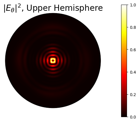
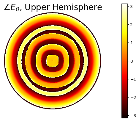
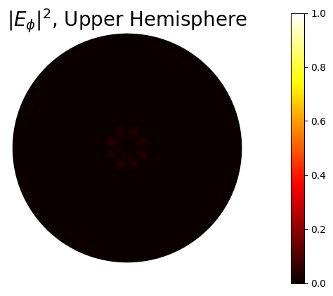
print(f"Q:{result['Q']}")
print(f"V:{result['V']}")
print(f"Pd:{result['Pd']}")
print(f"U:{result['U']}")
print(f"power overlap:{np.abs(result['overlap']) ** 2}")
Q:[6.13158041]
V:<xarray.DataArray ()> Size: 8B
array(8.43584096e-19)
Pd:2.6204282884204066e-13
U:[1.1095572e-27]
power overlap:[0.21122735]