Author: Hamish Carr Delgado, Stanford University.
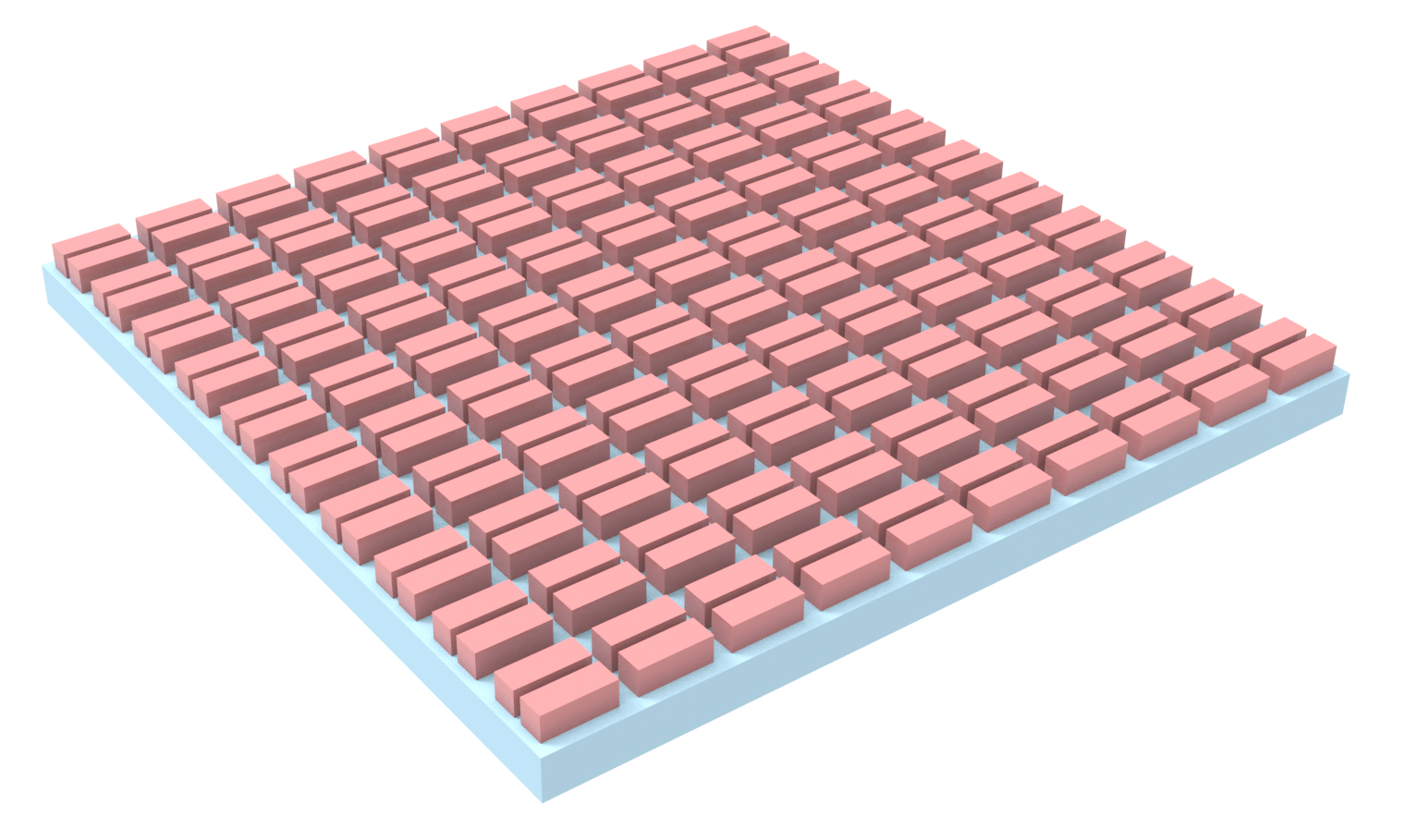
This tutorial builds a phase-gradient metasurface workflow in Tidy3D, starting from a single nanobar unit cell and ending with a fully 3D notched supercell that supports a resonant guided-mode response. The goal is to connect the physical design logic — phase coverage, supercell construction, guided-mode identification, and symmetry breaking — to a simulation-ready beam-steering metasurface example.
The design is based on the following papers:
Nonreciprocal Flat Optics with Silicon Metasurfaces Mark Lawrence, David R. Barton III, Jennifer A. Dionne Nano Letters (2018) https://pubs.acs.org/doi/abs/10.1021/acs.nanolett.7b04646
High quality factor phase gradient metasurfaces Mark Lawrence, David R. Barton III, Jefferson Dixon, Jung-Hwan Song, Jorik van de Groep, Mark L. Brongersma, Jennifer A. Dionne Nature Nanotechnology (2020) https://www.nature.com/articles/s41565-020-0754-x
The notebook is organized as a progressive design study. We first establish phase control in a simple dielectric bar library, then assemble a phase-gradient supercell, identify the underlying guided mode in the widest bar, perturb that mode with a notch, and finally simulate the full 3D notched supercell to recover the resonant diffraction response and field profile.
Tutorial Roadmap
The tutorial is organized into six sections:
- Unit-cell transmission and phase response. Sweep the width of a dielectric nanobar unit cell and extract transmission amplitude and phase to build a design library.
- Choosing a phase triplet for beam steering. Select three bar widths whose transmitted phases span a (2\pi) ramp in steps of (2\pi/3) with high transmission.
- Building and testing a three-bar phase-gradient supercell. Assemble the chosen widths into a supercell and verify that the structure redirects light into the (\pm 1) diffraction orders.
- Guided-mode analysis of the widest bar. Solve for the modes supported by the widest bar in a finite-width 3D configuration to identify the mode that will later be perturbed.
- Choosing the perturbation period and building the perturbed bar. Introduce a symmetry-breaking notch in the widest bar and verify resonant coupling to the guided mode in a 3D simulation.
- High-Q phase-gradient metasurface with periodic perturbations. Insert the notched widest bar back into the supercell, extract the resonant wavelength from the diffraction response, and visualize the resonant guided-mode profile.
Physical Picture
A silicon nanobar behaves in two useful ways. First, when illuminated at normal incidence, its width controls the complex transmission coefficient, so a width sweep can be used to build a phase library for metasurface design. Second, the same bar also supports guided modes, which normally couple only weakly to free-space radiation.
A phase-gradient metasurface uses several bar widths that provide different transmitted phases while maintaining high transmission. Repeating a supercell made of those widths creates a transverse phase ramp, which redirects light into a nonzero diffraction order.
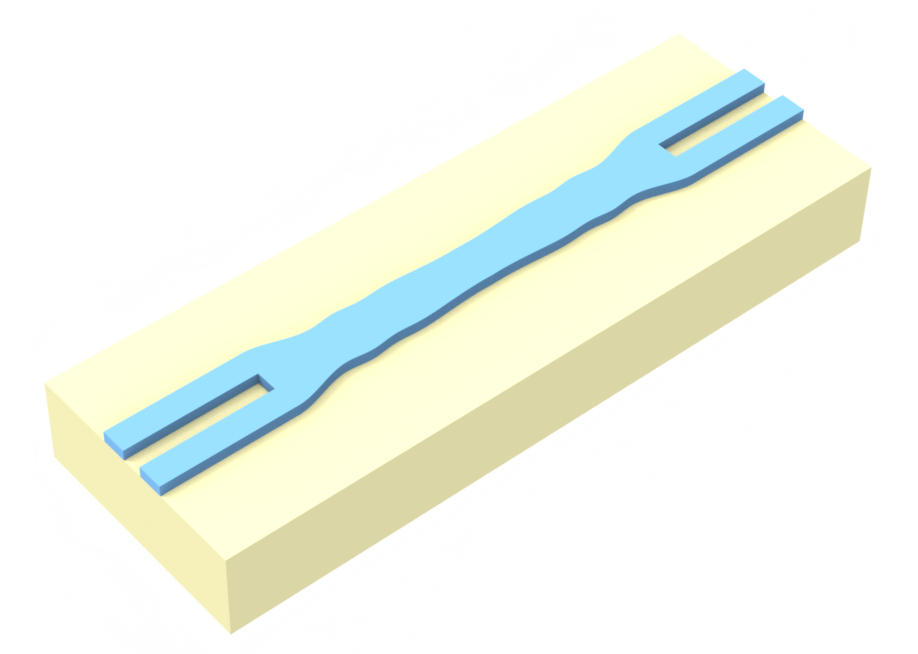
To obtain a high-Q response, we then add a weak periodic perturbation along the bar. This perturbation supplies the momentum and symmetry breaking needed to couple an incident plane wave into a guided mode. Because the perturbation can be kept small, the resonant leakage rate remains weak, producing a narrow linewidth and large quality factor.
import numpy as np
import matplotlib.pyplot as plt
import tidy3d as td
import tidy3d.web as web
from tidy3d.plugins.mode import ModeSolver
14:12:43 -03 WARNING: Using canonical configuration directory at
             '/home/filipe/.config/tidy3d'. Found legacy directory at
             '~/.tidy3d', which will be ignored. Remove it manually or run
             'tidy3d config migrate --delete-legacy' to clean up.
Common Parameters
We define the material system, wavelength range, and geometric scales once at the top of the notebook. This reduces redundancy and makes it easier to compare the unperturbed and perturbed designs on equal footing. The silicon bar and sapphire substrate are described by Medium objects with constant permittivities.
# Optical and spectral settings
lambda0 = 1.50 * um
freq0 = td.C_0 / lambda0
bandwidth = 0.20 * freq0
num_freqs = 101
freqs = np.linspace(freq0 - bandwidth / 2, freq0 + bandwidth / 2, num_freqs)

# Materials
si = td.Medium(permittivity=3.48**2, name="Si")
sapphire = td.Medium(permittivity=1.75**2, name="sapphire")
air = td.Medium(permittivity=1.0, name="air")

# Unit-cell geometry
h_bar = 0.70 * um
p_bar = 0.707 * um
sub_t = 5.0 * um
pml_t = 1.00 * um

# Grid / runtime
run_time = 2e-12
Helper Functions
The functions below provide a clean separation between geometry construction and simulation setup. The same conventions are reused for the unit-cell, supercell, and perturbed-bar simulations. They build the Structure objects for the bar and substrate, together with the PlaneWave source and the DiffractionMonitor, FluxMonitor, and FieldMonitor monitors used throughout the notebook.
# Example source and monitors for the 2D unit-cell simulations

source = td.PlaneWave(
    source_time=td.GaussianPulse(freq0=freq0, fwidth=bandwidth),
    size=(td.inf, td.inf, 0),
    center=(0, 0, -2),
    direction="+",
    pol_angle=0,
    name="planewave",
)

monitor_t = td.DiffractionMonitor(
    center=(0, 0, 1.5),
    size=(td.inf, td.inf, 0),
    freqs=[freq0],
    name="t",
)

T_monitor = td.FluxMonitor(
    center=(0, 0, 3),
    size=(td.inf, td.inf, 0),
    freqs=freqs,
    name="Transmission",
)

R_monitor = td.FluxMonitor(
    center=(0, 0, -3),
    size=(td.inf, td.inf, 0),
    freqs=freqs,
    name="Reflection",
)

xz_field = td.FieldMonitor(
    center=(0, 0, 0),
    size=(td.inf, 0, 3),
    fields=["Ex", "Ey", "Ez", "Hx", "Hy", "Hz"],
    freqs=[freq0],
    name="XZ field",
    colocate=True,
)


def make_substrate(period_x, period_y=td.inf, sub_t=sub_t):
    return td.Structure(
        geometry=td.Box(
            center=(0, 0, -sub_t / 2),
            size=(td.inf, td.inf, sub_t),
        ),
        medium=sapphire,
        name="substrate",
    )


def make_bar(width, center=(0, 0, h_bar / 2), length=td.inf, height=h_bar):
    return td.Structure(
        geometry=td.Box(center=center, size=(width, length, height)),
        medium=si,
        name=f"bar_w_{width:.3f}",
    )


def make_unit_cell(width, period=p_bar):
    return make_bar(width=width, length=td.inf)


def make_unit_cell_sim(width, period=p_bar, dl=0.02):
    sim_size_2d = (period, 0, sub_t + h_bar + 2 * pml_t)

    sim = td.Simulation(
        center=(0, 0, 0),
        size=sim_size_2d,
        grid_spec=td.GridSpec.uniform(dl=dl),
        structures=[
            make_unit_cell(width, period=period),
            make_substrate(period_x=period),
        ],
        sources=[source],
        monitors=[monitor_t],
        run_time=5e-12,
        shutoff=1e-7,
        boundary_spec=td.BoundarySpec(
            x=td.Boundary.periodic(),
            y=td.Boundary.periodic(),
            z=td.Boundary.pml(),
        ),
        symmetry=(0, 0, 0),
        medium=air,
    )
    return sim
1. Unit-Cell Transmission and Phase Response
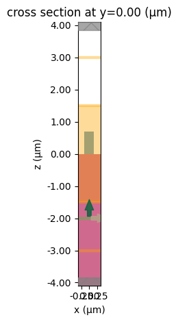
We first compute the complex transmission of a single periodic nanobar cell. The important quantity is the zeroth transmitted diffraction order, since that is the forward-propagating channel used to define the local phase response. We extract it from a DiffractionMonitor placed above the bar.
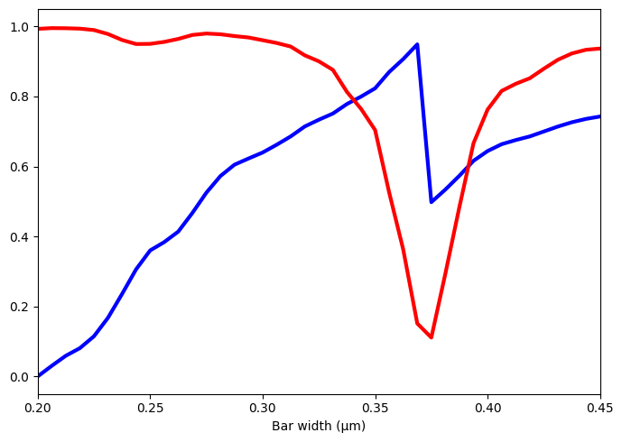
In practice, we sweep the bar width and extract both the amplitude and phase of the transmitted field. The width sweep is launched in parallel using a Batch, and the resulting phase library is later used to choose widths for a phase-gradient supercell.
example_width = 0.30 * um
sim_size_2d = (p_bar, 0, sub_t + h_bar + 2 * pml_t)

bar = make_bar(example_width, length=td.inf)
substrate = make_substrate(period_x=p_bar)

sim_uc = td.Simulation(
    center=(0, 0, 0),
    size=sim_size_2d,
    grid_spec=td.GridSpec.uniform(dl=0.02),
    structures=[bar, substrate],
    sources=[source],
    monitors=[T_monitor, R_monitor, xz_field],
    run_time=run_time,
    shutoff=1e-7,
    boundary_spec=td.BoundarySpec(
        x=td.Boundary.periodic(),
        y=td.Boundary.periodic(),
        z=td.Boundary.pml(),
    ),
    symmetry=(0, 0, 0),
    medium=air,
)

sim_uc.plot(y=0)
plt.show()
widths = np.linspace(0.20, 0.45, 41) * um

batch = web.Batch(simulations={f"w_{w:.4f}": make_unit_cell_sim(w) for w in widths})
batch_data = batch.run(path_dir="data/unit_cell_width_sweep")

t = np.zeros(len(widths), dtype=complex)

for i, w in enumerate(widths):
    data = batch_data[f"w_{w:.4f}"]
    t[i] = data["t"].amps.sel(f=freq0, orders_x=0, orders_y=0, polarization="p").item()

amps = np.abs(t)
theta = np.unwrap(np.angle(t))
theta = theta - theta[0]
theta_norm = theta / (2 * np.pi)
Output()
14:12:59 -03 Started working on Batch containing 41 tasks.
14:14:02 -03 Maximum FlexCredit cost: 1.025 for the whole batch.
             Use 'Batch.real_cost()' to get the billed FlexCredit cost after
             completion.
Output()
14:14:25 -03 Batch complete.
plt.figure(figsize=(7, 5))
plt.plot(widths / um, theta_norm, linewidth=3, c="blue")
plt.plot(widths / um, amps, linewidth=3, c="red")

plt.xlabel("Bar width (µm)")
plt.xlim(widths[0] / um, widths[-1] / um)
plt.ylim(-0.05, 1.05)
plt.yticks(np.linspace(0, 1, 6))
plt.tight_layout()
plt.show()
2. Choosing a Phase Triplet for Beam Steering
A phase-gradient metasurface redirects light by imposing a transverse phase discontinuity, as described by the generalized Snell's law framework introduced by Yu et al. [Science 2011]. For a linear phase profile, the metasurface behaves like a blazed grating: a total phase ramp of (2\pi) across one supercell period (\Lambda) preferentially redirects light into a nonzero diffraction order.
To couple the transmitted field mainly into the (\pm 1) diffraction order at the design wavelength, we choose a supercell period of approximately (\Lambda = 2121) nm. Dividing this into three equal subcells gives (p_{\mathrm{bar}} = \Lambda/3 = 707) nm per bar, so neighboring bars should differ in transmitted phase by (2\pi/3) to span a full (2\pi) ramp across the supercell.
With this choice, three bar widths from the unit-cell sweep act as a compact phase library: each supercell approximates a linear phase ramp, and repeating it across the surface directs light into the desired first diffraction order.
We now search the width sweep for triplets that satisfy two conditions:
- The transmitted phases are close to three evenly spaced values separated by (2\pi/3).
- The transmission amplitudes of all three bars exceed a chosen threshold.
After finding all valid triplets, we rank them by mean amplitude, minimum amplitude, or the product of amplitudes. This makes it easy to pick a set of widths that provides both good phase coverage and strong transmission.
import numpy as np
import matplotlib.pyplot as plt

phase = np.mod(theta, 2 * np.pi)
amp = np.abs(t)
w_list = widths / um

dphi_target = 2 * np.pi / 3
phase_tol = 0.05 * 2 * np.pi
amp_thresh = 0.8

triplet_data = []
seen = set()

for i0 in range(len(phase)):
    phi0 = phase[i0]

    phi1_target = np.mod(phi0 + dphi_target, 2 * np.pi)
    phi2_target = np.mod(phi0 + 2 * dphi_target, 2 * np.pi)

    dphi1 = np.angle(np.exp(1j * (phase - phi1_target)))
    dphi2 = np.angle(np.exp(1j * (phase - phi2_target)))

    cand1 = np.where(np.abs(dphi1) < phase_tol)[0]
    cand2 = np.where(np.abs(dphi2) < phase_tol)[0]

    if cand1.size == 0 or cand2.size == 0:
        continue

    i1 = int(cand1[np.argmin(np.abs(dphi1[cand1]))])
    i2 = int(cand2[np.argmin(np.abs(dphi2[cand2]))])

    idx_trip = tuple(sorted([i0, i1, i2]))

    if len(set(idx_trip)) < 3 or idx_trip in seen:
        continue
    seen.add(idx_trip)

    amps_trip = amp[list(idx_trip)]
    phases_trip = phase[list(idx_trip)]

    if np.all(amps_trip > amp_thresh):
        triplet_data.append(
            {
                "indices": idx_trip,
                "w": w_list[list(idx_trip)],
                "amp": amps_trip,
                "phase_norm": phases_trip / (2 * np.pi),
                "mean_amp": np.mean(amps_trip),
                "min_amp": np.min(amps_trip),
                "prod_amp": np.prod(amps_trip),
            }
        )

best_by_mean = sorted(triplet_data, key=lambda x: x["mean_amp"], reverse=True)
best_by_min = sorted(triplet_data, key=lambda x: x["min_amp"], reverse=True)
best_by_prod = sorted(triplet_data, key=lambda x: x["prod_amp"], reverse=True)

print(f"Found {len(triplet_data)} valid triplets\n")

print("Top 10 triplets by mean amplitude:")
for item in best_by_mean[:10]:
    print(
        f"indices={item['indices']}, "
        f"w={np.round(item['w'], 4)}, "
        f"amp={np.round(item['amp'], 4)}, "
        f"phase/2pi={np.round(item['phase_norm'], 4)}, "
        f"mean={item['mean_amp']:.4f}, "
        f"min={item['min_amp']:.4f}, "
        f"prod={item['prod_amp']:.4f}"
    )

# Choose one candidate, matching the previous notebook style
best = best_by_mean[9]
idx_trip = np.array(best["indices"])
w_trip = w_list[idx_trip]

phase_norm = np.mod(theta, 2 * np.pi) / (2 * np.pi)
amp = np.abs(t)

fig, ax_phase = plt.subplots(figsize=(6, 4))

color_phase = "C0"
color_amp = "C1"

ax_phase.plot(
    w_list,
    phase_norm,
    color=color_phase,
    lw=2,
    label="Phase / 2π",
)

ax_phase.plot(
    w_trip,
    phase_norm[idx_trip],
    linestyle="none",
    marker="o",
    markersize=8,
    markeredgecolor="k",
    markerfacecolor=color_phase,
    label="bar widths",
)

ax_phase.set_xlabel("w (µm)")
ax_phase.set_ylabel("Phase / 2π", color=color_phase)
ax_phase.tick_params(axis="y", labelcolor=color_phase)

ax_amp = ax_phase.twinx()
ax_amp.plot(
    w_list,
    amp,
    color=color_amp,
    lw=2,
    ls="--",
    label="|t|",
)
ax_amp.set_ylabel("|t|", color=color_amp)
ax_amp.tick_params(axis="y", labelcolor=color_amp)
ax_amp.set_ylim(0, 1.05 * amp.max())

lines_phase, labels_phase = ax_phase.get_legend_handles_labels()
lines_amp, labels_amp = ax_amp.get_legend_handles_labels()
ax_phase.legend(lines_phase + lines_amp, labels_phase + labels_amp, loc="best")

fig.tight_layout()
plt.show()

print("Best triplet indices:", idx_trip)
print("Best triplet w:", w_trip)
print("Best triplet |t|:", amp[idx_trip])
print("Best triplet phase/2π:", phase_norm[idx_trip])
Found 15 valid triplets

Top 10 triplets by mean amplitude:
indices=(0, 7, 17), w=[0.2    0.2438 0.3062], amp=[0.9933 0.95   0.9529], phase/2pi=[0.     0.3061 0.6622], mean=0.9654, min=0.9500, prod=0.8992
indices=(3, 10, 40), w=[0.2188 0.2625 0.45  ], amp=[0.9939 0.9646 0.937 ], phase/2pi=[0.0808 0.414  0.7429], mean=0.9652, min=0.9370, prod=0.8983
indices=(2, 10, 39), w=[0.2125 0.2625 0.4438], amp=[0.9951 0.9646 0.9336], phase/2pi=[0.0591 0.414  0.736 ], mean=0.9644, min=0.9336, prod=0.8960
indices=(1, 8, 18), w=[0.2062 0.25   0.3125], amp=[0.9954 0.9505 0.9427], phase/2pi=[0.0303 0.3601 0.686 ], mean=0.9629, min=0.9427, prod=0.8919
indices=(2, 9, 38), w=[0.2125 0.2563 0.4375], amp=[0.9951 0.956  0.9231], phase/2pi=[0.0591 0.3839 0.7264], mean=0.9581, min=0.9231, prod=0.8782
indices=(2, 9, 19), w=[0.2125 0.2563 0.3188], amp=[0.9951 0.956  0.9176], phase/2pi=[0.0591 0.3839 0.7144], mean=0.9562, min=0.9176, prod=0.8730
indices=(2, 10, 20), w=[0.2125 0.2625 0.325 ], amp=[0.9951 0.9646 0.9006], phase/2pi=[0.0591 0.414  0.7336], mean=0.9534, min=0.9006, prod=0.8644
indices=(2, 9, 37), w=[0.2125 0.2563 0.4312], amp=[0.9951 0.956  0.905 ], phase/2pi=[0.0591 0.3839 0.7141], mean=0.9520, min=0.9050, prod=0.8610
indices=(3, 10, 21), w=[0.2188 0.2625 0.3313], amp=[0.9939 0.9646 0.876 ], phase/2pi=[0.0808 0.414  0.7514], mean=0.9448, min=0.8760, prod=0.8398
indices=(1, 8, 36), w=[0.2062 0.25   0.425 ], amp=[0.9954 0.9505 0.8794], phase/2pi=[0.0303 0.3601 0.7   ], mean=0.9417, min=0.8794, prod=0.8320
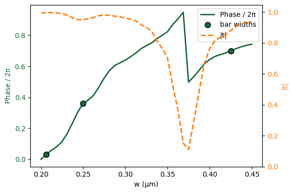
Best triplet indices: [ 1  8 36]
Best triplet w: [0.20625 0.25    0.425  ]
Best triplet |t|: [0.99543214 0.95045022 0.87935738]
Best triplet phase/2π: [0.03031425 0.36010208 0.69998862]
3. Building and Testing a Three-Bar Phase-Gradient Supercell
Once a suitable triplet of bar widths has been selected, we can combine the three unit cells into a single supercell. Repeating this supercell along the metasurface imposes a discrete approximation to a linear phase ramp, which should redirect transmitted light into a nonzero diffraction order.
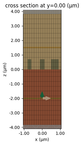
Here we construct a three-bar supercell with period (3p_{\mathrm{bar}}), using the selected widths in neighboring cells. We then simulate the structure and examine the transmitted diffraction efficiencies as a function of wavelength. If the phase-gradient design is working as intended, most of the transmitted power should be directed into one of the first diffraction orders rather than remaining in the zeroth order.
def make_3bar_unit_cell_sim(w1, w2, w3, dl=0.02):
    sim_size_3bar = (3 * p_bar, 0, sub_t + h_bar + 2 * pml_t)

    monitor_t_3bar = td.DiffractionMonitor(
        center=(0, 0, 1.5),
        size=(td.inf, td.inf, 0),
        freqs=freqs,
        name="t",
    )

    xz_field_3bar = td.FieldMonitor(
        center=(0, 0, 0),
        size=(td.inf, 0, td.inf),
        fields=["Ex", "Ey", "Ez", "Hx", "Hy", "Hz"],
        freqs=freqs,
        name="xz_field",
        colocate=True,
    )

    structures = [
        make_bar(w1, center=(-p_bar, 0, h_bar / 2), length=td.inf),
        make_bar(w2, center=(0.0, 0, h_bar / 2), length=td.inf),
        make_bar(w3, center=(p_bar, 0, h_bar / 2), length=td.inf),
        make_substrate(period_x=3 * p_bar),
    ]

    sim = td.Simulation(
        center=(0, 0, 0),
        size=sim_size_3bar,
        grid_spec=td.GridSpec.uniform(dl=dl),
        structures=structures,
        sources=[source],
        monitors=[monitor_t_3bar, xz_field_3bar],
        run_time=5e-12,
        shutoff=1e-7,
        boundary_spec=td.BoundarySpec(
            x=td.Boundary.periodic(),
            y=td.Boundary.periodic(),
            z=td.Boundary.pml(),
        ),
        symmetry=(0, 0, 0),
        medium=air,
    )
    return sim
w1, w2, w3 = best["w"]
sim_3bar = make_3bar_unit_cell_sim(w1, w2, w3)

ax = sim_3bar.plot(y=0)
sim_3bar.plot_grid(y=0, ax=ax)
ax.set_aspect(0.8)
plt.show()
sim_3bar_data = web.run(
    sim_3bar,
    task_name="3bar_sim",
    path="data/tutorial/3bar_sim.hdf5",
)
14:14:50 -03 Created task '3bar_sim' with resource_id
             'fdve-9bc35d3f-338b-49fa-bd9e-8a7088be6b3d' and task_type 'FDTD'.
             View task using web UI at
             'https://tidy3d.simulation.cloud/workbench?taskId=fdve-9bc35d3f-338
             b-49fa-bd9e-8a7088be6b3d'.
Task folder: 'default'.
Output()
14:14:53 -03 Estimated FlexCredit cost: 0.025. Minimum cost depends on task
             execution details. Use 'web.real_cost(task_id)' to get the billed
             FlexCredit cost after a simulation run.
14:14:55 -03 status = queued
             To cancel the simulation, use 'web.abort(task_id)' or
             'web.delete(task_id)' or abort/delete the task in the web UI.
             Terminating the Python script will not stop the job running on the
             cloud.
Output()
14:15:05 -03 starting up solver
running solver
Output()
14:15:16 -03 early shutoff detected at 57%, exiting.
14:15:17 -03 status = postprocess
Output()
14:15:23 -03 status = success
14:15:25 -03 View simulation result at
             'https://tidy3d.simulation.cloud/workbench?taskId=fdve-9bc35d3f-338
             b-49fa-bd9e-8a7088be6b3d'.
Output()
14:15:34 -03 Loading results from data/tutorial/3bar_sim.hdf5
import numpy as np
import matplotlib.pyplot as plt

diff_t = sim_3bar_data["t"]

freqs_3bar = np.asarray(diff_t.f)
lams = td.constants.C_0 / freqs_3bar
lams_um = lams

amps = diff_t.amps
amps_p = amps.sel(polarization="p")
eta_p = np.abs(amps_p) ** 2

try:
    eta_p_1d = eta_p.squeeze("orders_y")
except Exception:
    eta_p_1d = eta_p

orders_x = np.asarray(eta_p_1d.coords["orders_x"])

fig, ax = plt.subplots(figsize=(6, 4))

for m in orders_x:
    eta_m = np.asarray(eta_p_1d.sel(orders_x=m))
    ax.plot(lams_um, eta_m, label=f"m = {m}")

ax.set_xlabel("Wavelength (µm)")
ax.set_ylabel("Diffraction efficiency (p-pol)")
ax.set_title("Transmitted diffraction efficiency vs wavelength")
ax.legend(title="Order", bbox_to_anchor=(1.05, 1), loc="upper left")
ax.set_ylim(0, 1.05 * np.max(np.asarray(eta_p_1d)))

fig.tight_layout()
plt.show()
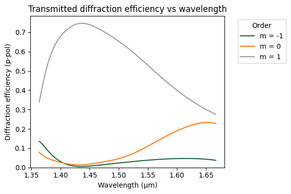
The result confirms that the three-bar supercell functions as a beam-steering metasurface. Instead of transmitting mostly into the zeroth order, the structure redirects most of the transmitted power into one of the first diffraction orders over a broad wavelength range. This verifies that the discrete phase ramp selected from the unit-cell phase library is sufficient to produce the intended anomalous refraction behavior.
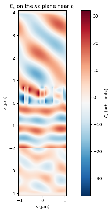
We can also inspect the near-field distribution inside and above the supercell. The field profile on the (xz) plane shows how the three neighboring bars shape the transmitted wavefront and launch a tilted outgoing field. In particular, the phase ramp encoded by the three bar widths appears as a spatially varying field pattern above the metasurface, consistent with the redistribution of power into a nonzero diffraction order.
To make this more intuitive, we animate the real part of the complex field at a fixed frequency near (f_0). This phase sweep reconstructs the time-harmonic oscillation of the field and makes the steered transmitted wavefront easier to see than a single static snapshot.
xz = sim_3bar_data["xz_field"]

Ex_da = xz.Ex.sel(f=freq0, method="nearest").squeeze()

if Ex_da.dims == ("z", "x"):
    Ex_da = Ex_da.transpose("x", "z")

x = np.asarray(Ex_da.coords["x"])
z = np.asarray(Ex_da.coords["z"])
Ex_plot = np.real(np.asarray(Ex_da))

fig, ax = plt.subplots(figsize=(10, 7))
pcm = ax.pcolormesh(
    x,
    z,
    Ex_plot.T,
    shading="auto",
    cmap="RdBu_r",
)

ax.set_xlabel("x (µm)")
ax.set_ylabel("z (µm)")
ax.set_title(r"$E_x$ on the $xz$ plane near $f_0$")
ax.set_aspect("equal")

cbar = fig.colorbar(pcm, ax=ax)
cbar.set_label(r"$E_x$ (arb. units)")

fig.tight_layout()
plt.show()
from matplotlib.animation import FuncAnimation
from IPython.display import HTML

Ex_vals = np.asarray(Ex_da)
Ex_mag = np.abs(Ex_vals)
Ex_arg = np.angle(Ex_vals)

n_frames = 40
phases = np.linspace(0, 2 * np.pi, n_frames, endpoint=False)

fig, ax = plt.subplots(figsize=(6, 4))

Ex_frame = Ex_mag * np.cos(Ex_arg - phases[0])

pcm = ax.pcolormesh(
    x,
    z,
    Ex_frame.T,
    shading="auto",
    cmap="RdBu_r",
    vmin=-np.max(Ex_mag),
    vmax=np.max(Ex_mag),
)

ax.set_xlabel("x (µm)")
ax.set_ylabel("z (µm)")
ax.set_title(r"$\Re\{E_x\}$ on the $xz$ plane at $f_0$")
ax.set_aspect("equal")

cbar = fig.colorbar(pcm, ax=ax)
cbar.set_label(r"$\Re\{E_x\}$ (arb. units)")

fig.tight_layout()


def update(i):
    Ex_frame = Ex_mag * np.cos(Ex_arg - phases[i])
    pcm.set_array(Ex_frame.T.ravel())
    return (pcm,)


anim = FuncAnimation(
    fig,
    update,
    frames=n_frames,
    interval=80,
    blit=True,
)

plt.close(fig)
HTML(anim.to_jshtml())
4. Guided-Mode Analysis of the Widest Bar
The three-bar supercell demonstrates beam steering, but it does not yet explain how a high-(Q) resonance can be introduced. To build that part of the design, we next analyze the guided modes supported by one of the nanobars in the supercell using the ModeSolver plugin.
We focus on the widest bar in the selected triplet, since it typically supports the most strongly confined modes in this geometry. By solving for its guided modes, we can extract both the modal field profiles and the propagation constant (\beta), which together tell us how light propagates along the bar.
This information is essential because a guided mode cannot usually be excited directly from normal-incidence free-space illumination. To couple light into that mode, we must later add a weak periodic perturbation that supplies the missing momentum. The required perturbation period is set by the guided wavelength (\lambda_g = 2\pi/\beta).
lams_mode = np.arange(1.45, 1.55 + 1e-9, 0.01)
freqs_mode = td.C_0 / lams_mode

w1, w2, w3 = best["w"]

Lx_mode = 6 * w3
Lz_mode = sub_t + h_bar + 2 * pml_t

wg_core = td.Structure(
    geometry=td.Box(center=(0, 0, h_bar / 2), size=(w3, td.inf, h_bar)),
    medium=si,
    name="wg_core",
)

wg_substrate = td.Structure(
    geometry=td.Box(
        center=(0, 0, -sub_t / 2),
        size=(td.inf, td.inf, sub_t),
    ),
    medium=sapphire,
    name="wg_substrate",
)

sim_mode = td.Simulation(
    center=(0, 0, 0),
    size=(Lx_mode, 0, Lz_mode),
    grid_spec=td.GridSpec.uniform(dl=0.02),
    structures=[wg_core, wg_substrate],
    sources=[],
    monitors=[],
    run_time=1e-12,
    boundary_spec=td.BoundarySpec(
        x=td.Boundary.pml(),
        y=td.Boundary.periodic(),
        z=td.Boundary.pml(),
    ),
    symmetry=(0, 0, 0),
    medium=air,
)

mode_spec = td.ModeSpec(
    num_modes=4,
    target_neff=2.7,
)

plane = td.Box(
    center=(0, 0, 0),
    size=(Lx_mode, 0, Lz_mode),
)

mode_solver = ModeSolver(
    simulation=sim_mode,
    plane=plane,
    mode_spec=mode_spec,
    freqs=freqs_mode,
)

mode_data = mode_solver.solve()
mode_data.to_dataframe()
14:15:38 -03 WARNING: Use the remote mode solver with subpixel averaging for
             better accuracy through 'tidy3d.web.run(...)' or the deprecated
             'tidy3d.plugins.mode.web.run(...)'. Alternatively, you can install
             the package 'tidy3d-extras' using 'pip install "tidy3d"' and set
             'config.simulation.use_local_subpixel=True'.
| wavelength | n eff | k eff | loss (dB/cm) | TE (Ex) fraction | wg TE fraction | wg TM fraction | mode area | ||
|---|---|---|---|---|---|---|---|---|---|
| f | mode_index | ||||||||
| 2.067534e+14 | 0 | 1.45 | 3.071280 | 0.0 | 0.0 | 0.001525 | 0.901049 | 0.899968 | 0.222209 |
| 1 | 1.45 | 2.927399 | 0.0 | 0.0 | 0.990738 | 0.723665 | 0.948246 | 0.288919 | |
| 2 | 1.45 | 2.546938 | 0.0 | 0.0 | 0.874179 | 0.794376 | 0.747433 | 0.332909 | |
| 3 | 1.45 | 2.546307 | 0.0 | 0.0 | 0.015817 | 0.652361 | 0.917692 | 0.344248 | |
| 2.053373e+14 | 0 | 1.46 | 3.066298 | 0.0 | 0.0 | 0.001576 | 0.899598 | 0.899149 | 0.223469 |
| 1 | 1.46 | 2.919543 | 0.0 | 0.0 | 0.990453 | 0.720415 | 0.947682 | 0.291697 | |
| 2 | 1.46 | 2.533974 | 0.0 | 0.0 | 0.870152 | 0.793691 | 0.743615 | 0.337302 | |
| 3 | 1.46 | 2.533062 | 0.0 | 0.0 | 0.016546 | 0.648753 | 0.917310 | 0.347876 | |
| 2.039404e+14 | 0 | 1.47 | 3.061292 | 0.0 | 0.0 | 0.001629 | 0.898137 | 0.898331 | 0.224744 |
| 1 | 1.47 | 2.911622 | 0.0 | 0.0 | 0.990161 | 0.717166 | 0.947117 | 0.294510 | |
| 2 | 1.47 | 2.520921 | 0.0 | 0.0 | 0.866047 | 0.793076 | 0.739751 | 0.341775 | |
| 3 | 1.47 | 2.519713 | 0.0 | 0.0 | 0.017309 | 0.645194 | 0.916939 | 0.351542 | |
| 2.025625e+14 | 0 | 1.48 | 3.056260 | 0.0 | 0.0 | 0.001683 | 0.896666 | 0.897516 | 0.226036 |
| 1 | 1.48 | 2.903638 | 0.0 | 0.0 | 0.989861 | 0.713920 | 0.946550 | 0.297358 | |
| 2 | 1.48 | 2.507780 | 0.0 | 0.0 | 0.861866 | 0.792533 | 0.735842 | 0.346330 | |
| 3 | 1.48 | 2.506262 | 0.0 | 0.0 | 0.018106 | 0.641688 | 0.916578 | 0.355246 | |
| 2.012030e+14 | 0 | 1.49 | 3.051204 | 0.0 | 0.0 | 0.001739 | 0.895185 | 0.896703 | 0.227343 |
| 1 | 1.49 | 2.895588 | 0.0 | 0.0 | 0.989554 | 0.710677 | 0.945981 | 0.300240 | |
| 2 | 1.49 | 2.494552 | 0.0 | 0.0 | 0.857610 | 0.792065 | 0.731887 | 0.350967 | |
| 3 | 1.49 | 2.492708 | 0.0 | 0.0 | 0.018939 | 0.638240 | 0.916228 | 0.358987 | |
| 1.998616e+14 | 0 | 1.50 | 3.046122 | 0.0 | 0.0 | 0.001796 | 0.893693 | 0.895892 | 0.228667 |
| 1 | 1.50 | 2.887474 | 0.0 | 0.0 | 0.989240 | 0.707439 | 0.945411 | 0.303158 | |
| 2 | 1.50 | 2.481237 | 0.0 | 0.0 | 0.853280 | 0.791670 | 0.727887 | 0.355686 | |
| 3 | 1.50 | 2.479054 | 0.0 | 0.0 | 0.019810 | 0.634854 | 0.915890 | 0.362766 | |
| 1.985381e+14 | 0 | 1.51 | 3.041016 | 0.0 | 0.0 | 0.001855 | 0.892192 | 0.895084 | 0.230008 |
| 1 | 1.51 | 2.879295 | 0.0 | 0.0 | 0.988917 | 0.704205 | 0.944839 | 0.306110 | |
| 2 | 1.51 | 2.467837 | 0.0 | 0.0 | 0.848879 | 0.791352 | 0.723841 | 0.360487 | |
| 3 | 1.51 | 2.465300 | 0.0 | 0.0 | 0.020719 | 0.631534 | 0.915562 | 0.366583 | |
| 1.972319e+14 | 0 | 1.52 | 3.035885 | 0.0 | 0.0 | 0.001916 | 0.890681 | 0.894278 | 0.231365 |
| 1 | 1.52 | 2.871050 | 0.0 | 0.0 | 0.988586 | 0.700976 | 0.944265 | 0.309097 | |
| 2 | 1.52 | 2.454351 | 0.0 | 0.0 | 0.844410 | 0.791111 | 0.719750 | 0.365372 | |
| 3 | 1.52 | 2.451446 | 0.0 | 0.0 | 0.021670 | 0.628286 | 0.915246 | 0.370438 | |
| 1.959428e+14 | 0 | 1.53 | 3.030730 | 0.0 | 0.0 | 0.001978 | 0.889160 | 0.893475 | 0.232740 |
| 1 | 1.53 | 2.862739 | 0.0 | 0.0 | 0.988247 | 0.697754 | 0.943690 | 0.312118 | |
| 2 | 1.53 | 2.440782 | 0.0 | 0.0 | 0.839874 | 0.790947 | 0.715614 | 0.370339 | |
| 3 | 1.53 | 2.437493 | 0.0 | 0.0 | 0.022662 | 0.625113 | 0.914941 | 0.374332 | |
| 1.946704e+14 | 0 | 1.54 | 3.025549 | 0.0 | 0.0 | 0.002042 | 0.887629 | 0.892675 | 0.234132 |
| 1 | 1.54 | 2.854362 | 0.0 | 0.0 | 0.987900 | 0.694540 | 0.943113 | 0.315174 | |
| 2 | 1.54 | 2.427129 | 0.0 | 0.0 | 0.835274 | 0.790862 | 0.711433 | 0.375391 | |
| 3 | 1.54 | 2.423444 | 0.0 | 0.0 | 0.023699 | 0.622021 | 0.914649 | 0.378265 | |
| 1.934145e+14 | 0 | 1.55 | 3.020344 | 0.0 | 0.0 | 0.002108 | 0.886089 | 0.891877 | 0.235541 |
| 1 | 1.55 | 2.845919 | 0.0 | 0.0 | 0.987544 | 0.691333 | 0.942535 | 0.318264 | |
| 2 | 1.55 | 2.413395 | 0.0 | 0.0 | 0.830614 | 0.790856 | 0.707208 | 0.380525 | |
| 3 | 1.55 | 2.409299 | 0.0 | 0.0 | 0.024781 | 0.619016 | 0.914368 | 0.382238 |
We begin by plotting the first few modal field profiles at a representative wavelength near (1.5) µm. These mode shapes help us identify the character of the supported guided modes and distinguish the dominant fundamental-like solutions from higher-order ones.
lam_plot = 1.50
f0_ind = np.argmin(np.abs(lams_mode - lam_plot))
num_modes_plot = 4

fig, axes = plt.subplots(
    num_modes_plot,
    2,
    figsize=(10, 6 * num_modes_plot),
    tight_layout=True,
)

for m in range(num_modes_plot):
    abs(mode_data.Ex.isel(mode_index=m, f=f0_ind)).plot(
        x="x",
        y="z",
        ax=axes[m, 0],
        cmap="magma",
        add_colorbar=True,
    )
    abs(mode_data.Ez.isel(mode_index=m, f=f0_ind)).plot(
        x="x",
        y="z",
        ax=axes[m, 1],
        cmap="magma",
        add_colorbar=True,
    )

    axes[m, 0].set_title(f"Mode {m}: |Ex| at λ = {lams_mode[f0_ind]:.2f} µm")
    axes[m, 0].set_aspect("equal")

    axes[m, 1].set_title(f"Mode {m}: |Ez| at λ = {lams_mode[f0_ind]:.2f} µm")
    axes[m, 1].set_aspect("equal")

plt.show()
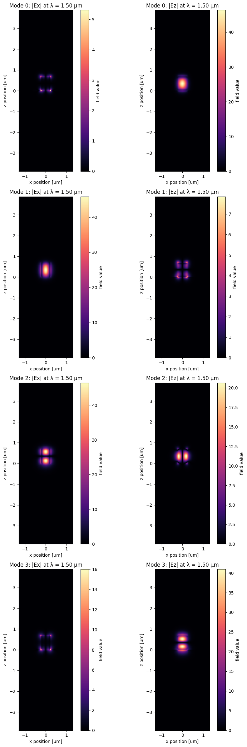
After identifying the guided modes, we examine their dispersion through the propagation constant (\beta). Here we focus on modes 0 and 1, which correspond most closely to the fundamental TE-like and TM-like guided modes of the bar. These are the most relevant modes for the perturbative high-(Q) design that follows.
n_eff_da = np.real(mode_data.n_eff)
f_mode = np.asarray(n_eff_da.coords["f"])
n_eff = np.asarray(n_eff_da)

lam_mode = td.C_0 / f_mode
beta = (2 * np.pi * f_mode[:, None] / td.C_0) * n_eff

modes_to_plot = [0, 1]

fig, ax = plt.subplots(figsize=(6, 4))

for m in modes_to_plot:
    ax.plot(lam_mode, beta[:, m], label=f"Mode {m}")

ax.set_xlabel("Wavelength (µm)")
ax.set_ylabel(r"$\beta$ (rad/µm)")
ax.set_title(r"Propagation constant $\beta$ vs wavelength")
ax.legend()
ax.grid(True, alpha=0.3)

plt.show()
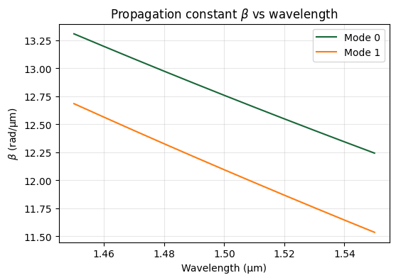
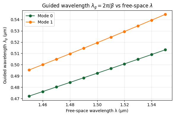
From the propagation constant, we can compute the guided wavelength (\lambda_g = 2\pi/\beta). This quantity sets the spatial scale of the longitudinal perturbation needed to phase-match the incident plane wave into the guided mode. In the next section, we use this result to choose the perturbation period for the resonant metasurface design.
lambda_g = 2 * np.pi / beta

modes_to_plot = [0, 1]

fig, ax = plt.subplots(figsize=(6, 4))

for m in modes_to_plot:
    ax.plot(lam_mode, lambda_g[:, m], marker="o", label=f"Mode {m}")

ax.set_xlabel("Free-space wavelength λ (µm)")
ax.set_ylabel(r"Guided wavelength $\lambda_g$ (µm)")
ax.set_title(r"Guided wavelength $\lambda_g = 2\pi/\beta$ vs free-space $\lambda$")
ax.legend()
ax.grid(True, alpha=0.3)

fig.tight_layout()
plt.show()
5. Choosing the Perturbation Period and Building the Perturbed Bar
The guided-mode calculation tells us how rapidly the phase of a supported mode accumulates along the bar. At a target free-space wavelength near (1.5) µm, the corresponding guided wavelength (\lambda_g) sets the longitudinal scale needed to couple incident light into that mode.
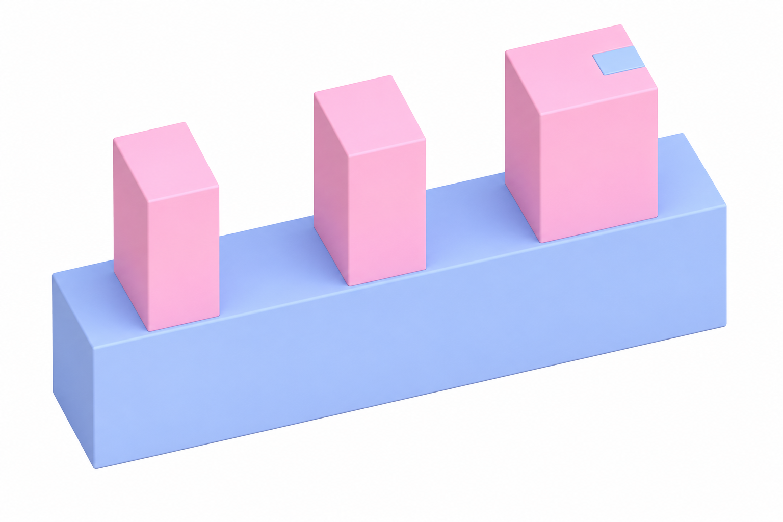
We now use that result to choose the period of a weak structural perturbation. In practice, we introduce a shallow notch and repeat it periodically along the (y) direction. This perturbation breaks the translational symmetry of the unperturbed bar and supplies the momentum needed to phase-match normally incident light into the guided mode.
To verify that this mechanism works, we first simulate a single perturbed bar in a 3D periodic cell. This isolates the resonance physics before we later return to the full phase-gradient metasurface.
lam_target = 1.50
i0 = np.argmin(np.abs(lam_mode - lam_target))

mode_index_target = 1
lambda_g_target = lambda_g[i0, mode_index_target]

print(f"Closest λ in grid: {lam_mode[i0]:.4f} µm")
print(
    f"Guided wavelength λ_g for mode {mode_index_target} at λ ≈ {lam_mode[i0]:.4f} µm: "
    f"{lambda_g_target:.4f} µm"
)
print(
    f"Based on the mode analysis, we choose a perturbation period of approximately "
    f"{lambda_g_target * 1000:.0f} nm to couple free-space light into the selected guided mode."
)
Closest λ in grid: 1.5000 µm
Guided wavelength λ_g for mode 1 at λ ≈ 1.5000 µm: 0.5195 µm
Based on the mode analysis, we choose a perturbation period of approximately 519 nm to couple free-space light into the selected guided mode.
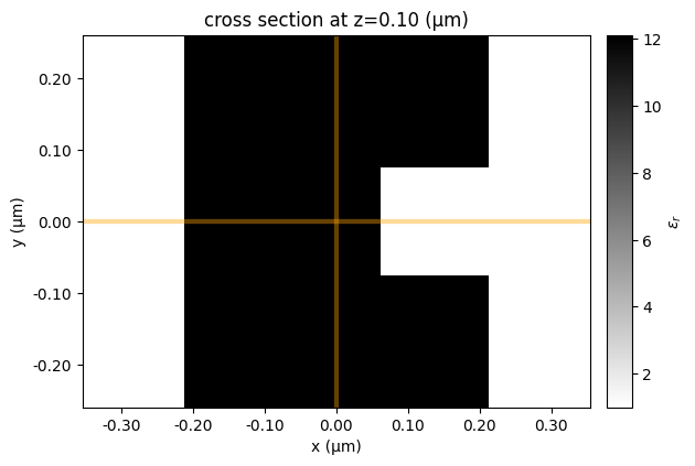
We now transition from the 2D phase-gradient picture to a 3D periodic simulation of a weakly perturbed bar. The unit cell is periodic in both (x) and (y): periodicity in (x) preserves the original metasurface period, while periodicity in (y) represents the repeated notch perturbation used to excite the guided mode.
The notch is designed to be weak, so that it enables coupling to the guided mode without strongly distorting the underlying bar geometry. This weak coupling is what allows the resonant leakage rate to remain small, leading to a narrow linewidth and a high quality factor.
w_bar = w3
p_notch = float(lambda_g_target)

w_notch = 0.15 * um
d_notch = 0.15 * um

wl_center = 1.50 * um
wl_band = 0.06 * um
wl_min = wl_center - wl_band / 2
wl_max = wl_center + wl_band / 2

freq0_3d = td.C_0 / wl_center
fwidth_3d = 0.5 * (td.C_0 / wl_min - td.C_0 / wl_max)

num_freqs_3d = 1001
monitor_freqs_3d = np.linspace(td.C_0 / wl_max, td.C_0 / wl_min, num_freqs_3d)
monitor_lambdas_3d = td.C_0 / monitor_freqs_3d

dl_3d = wl_min / (30 * np.sqrt(si.permittivity))
run_time_3d = 50e-12

print(f"Chosen perturbation period p_notch = {p_notch:.4f} µm")
print(f"Grid step dl = {dl_3d * 1000:.1f} nm")
Chosen perturbation period p_notch = 0.5195 µm
Grid step dl = 14.1 nm
def make_notched_bar_sim(
    w_bar,
    p_notch,
    w_notch=0.15 * um,
    d_notch=0.10 * um,
    dl=dl_3d,
    freqs=monitor_freqs_3d,
):
    bar = td.Structure(
        geometry=td.Box(
            center=(0, 0, h_bar / 2),
            size=(w_bar, td.inf, h_bar),
        ),
        medium=si,
        name="bar",
    )

    substrate = td.Structure(
        geometry=td.Box(
            center=(0, 0, -sub_t / 2),
            size=(td.inf, td.inf, sub_t),
        ),
        medium=sapphire,
        name="substrate",
    )

    notch = td.Structure(
        geometry=td.Box(
            center=(w_bar / 2 - d_notch / 2, 0, h_bar / 2),
            size=(d_notch, w_notch, h_bar),
        ),
        medium=air,
        name="notch",
    )

    source_3d = td.PlaneWave(
        source_time=td.GaussianPulse(freq0=freq0_3d, fwidth=fwidth_3d),
        size=(td.inf, td.inf, 0),
        center=(0, 0, -2.0),
        direction="+",
        pol_angle=0,
        name="planewave",
    )

    T_monitor_3d = td.FluxMonitor(
        center=(0, 0, 3.0),
        size=(td.inf, td.inf, 0),
        freqs=freqs,
        name="Transmission",
    )

    R_monitor_3d = td.FluxMonitor(
        center=(0, 0, -3.0),
        size=(td.inf, td.inf, 0),
        freqs=freqs,
        name="Reflection",
    )

    xz_field_3d = td.FieldMonitor(
        center=(0, 0, 0),
        size=(td.inf, 0, 3.0),
        fields=["Ex", "Ey", "Ez", "Hx", "Hy", "Hz"],
        freqs=freqs,
        name="xz_field",
        colocate=True,
    )

    xy_field_3d = td.FieldMonitor(
        center=(0, 0, h_bar / 2),
        size=(td.inf, td.inf, 0),
        fields=["Ex", "Ey", "Ez", "Hx", "Hy", "Hz"],
        freqs=freqs,
        name="xy_field",
        colocate=True,
    )

    yz_field_3d = td.FieldMonitor(
        center=(0, 0, 0),
        size=(0, td.inf, 3.0),
        fields=["Ex", "Ey", "Ez", "Hx", "Hy", "Hz"],
        freqs=freqs,
        name="yz_field",
        colocate=True,
    )

    sim_3d = td.Simulation(
        center=(0, 0, 0),
        size=(p_bar, p_notch, sub_t + h_bar + 2 * pml_t),
        grid_spec=td.GridSpec.uniform(dl=dl),
        structures=[bar, substrate, notch],
        sources=[source_3d],
        monitors=[T_monitor_3d, R_monitor_3d, xz_field_3d, xy_field_3d, yz_field_3d],
        run_time=run_time_3d,
        shutoff=1e-7,
        boundary_spec=td.BoundarySpec(
            x=td.Boundary.periodic(),
            y=td.Boundary.periodic(),
            z=td.Boundary.pml(),
        ),
        symmetry=(0, 0, 0),
        medium=air,
    )

    return sim_3d
sim_3d = make_notched_bar_sim(
    w_bar=w_bar,
    p_notch=p_notch,
    w_notch=w_notch,
    d_notch=d_notch,
)

sim_3d.plot_eps(z=0.1)
<Axes: title={'center': 'cross section at z=0.10 (μm)'}, xlabel='x (μm)', ylabel='y (μm)'>
sim_3d_data = web.run(
    sim_3d,
    task_name="3d_notched_bar",
    path="data/tutorial/3d_notched_bar.hdf5",
)
14:16:04 -03 WARNING: Simulation has 1.87e+06 time steps. The 'run_time' may be
             unnecessarily large, unless there are very long-lived resonances.
14:16:05 -03 Created task '3d_notched_bar' with resource_id
             'fdve-ab8f044f-d1c4-4482-a4e7-e1e030ad7d5c' and task_type 'FDTD'.
             View task using web UI at
             'https://tidy3d.simulation.cloud/workbench?taskId=fdve-ab8f044f-d1c
             4-4482-a4e7-e1e030ad7d5c'.
Task folder: 'default'.
Output()
14:16:08 -03 Estimated FlexCredit cost: 0.814. Minimum cost depends on task
             execution details. Use 'web.real_cost(task_id)' to get the billed
             FlexCredit cost after a simulation run.
14:16:10 -03 status = queued
             To cancel the simulation, use 'web.abort(task_id)' or
             'web.delete(task_id)' or abort/delete the task in the web UI.
             Terminating the Python script will not stop the job running on the
             cloud.
Output()
14:16:14 -03 status = preprocess
14:16:19 -03 starting up solver
14:16:20 -03 running solver
Output()
14:23:33 -03 early shutoff detected at 79%, exiting.
status = postprocess
Output()
14:24:10 -03 status = success
14:24:12 -03 View simulation result at
             'https://tidy3d.simulation.cloud/workbench?taskId=fdve-ab8f044f-d1c
             4-4482-a4e7-e1e030ad7d5c'.
Output()
14:25:06 -03 Loading results from data/tutorial/3d_notched_bar.hdf5
T = np.asarray(sim_3d_data["Transmission"].flux)
R = np.asarray(sim_3d_data["Reflection"].flux)

fig, (ax1, ax2) = plt.subplots(1, 2, figsize=(8, 4), tight_layout=True)

ax1.plot(monitor_lambdas_3d, np.abs(T), lw=2)
ax1.set_xlabel("Wavelength (µm)")
ax1.set_ylabel("Transmittance")
ax1.set_title("Transmission spectrum")

ax2.plot(monitor_lambdas_3d, np.abs(R), lw=2)
ax2.set_xlabel("Wavelength (µm)")
ax2.set_ylabel("Reflectance")
ax2.set_title("Reflection spectrum")

plt.show()
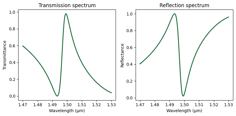
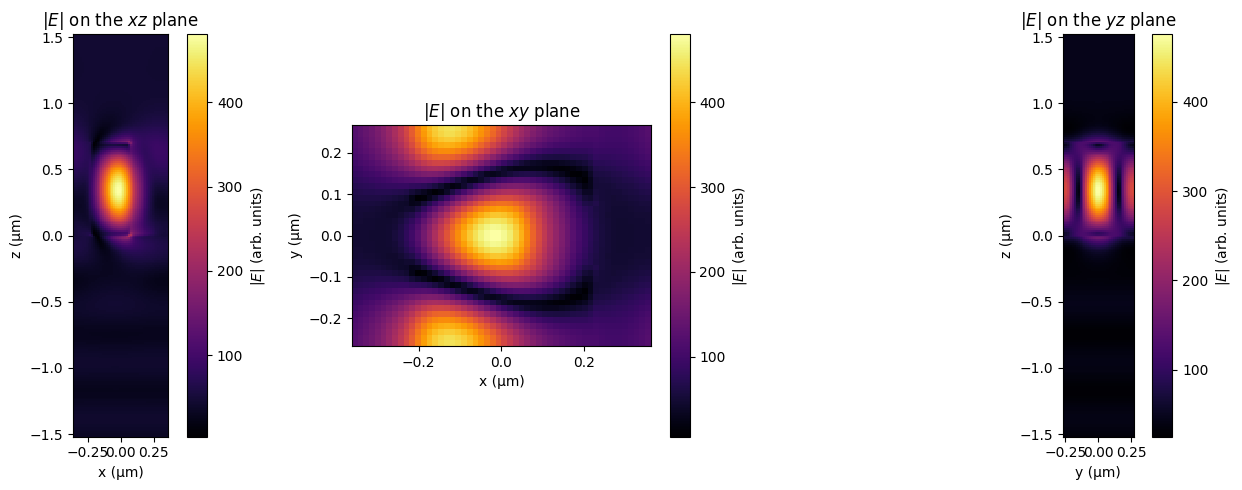
To confirm the resonant character of the perturbed bar, it is helpful to inspect the field distributions at the central wavelength. We plot the field magnitude on the (xz), (xy), and (yz) planes to visualize where the resonance is localized inside the bar, how strongly it interacts with the notch perturbation, and how it extends into the surrounding medium.
Together, these cross-sections provide a more complete picture of the guided-mode resonance than the spectrum alone. Strong field concentration near the bar and notch region is consistent with resonant excitation of a weakly radiative guided mode.
fig, axes = plt.subplots(1, 3, figsize=(14, 5), tight_layout=True)

# --- xz plane ---
xz = sim_3d_data["xz_field"]
Ex = xz.Ex.sel(f=freq0_3d, method="nearest").squeeze()
Ey = xz.Ey.sel(f=freq0_3d, method="nearest").squeeze()
Ez = xz.Ez.sel(f=freq0_3d, method="nearest").squeeze()
if Ex.dims == ("z", "x"):
    Ex, Ey, Ez = Ex.transpose("x", "z"), Ey.transpose("x", "z"), Ez.transpose("x", "z")
x = np.asarray(Ex.coords["x"])
z = np.asarray(Ex.coords["z"])
Eabs_xz = np.sqrt(
    np.abs(np.asarray(Ex)) ** 2
    + np.abs(np.asarray(Ey)) ** 2
    + np.abs(np.asarray(Ez)) ** 2
)
pcm0 = axes[0].pcolormesh(x, z, Eabs_xz.T, shading="auto", cmap="inferno")
axes[0].set_xlabel("x (µm)")
axes[0].set_ylabel("z (µm)")
axes[0].set_title(r"$|E|$ on the $xz$ plane")
axes[0].set_aspect("equal")
fig.colorbar(pcm0, ax=axes[0], label=r"$|E|$ (arb. units)")

# --- xy plane ---
xy = sim_3d_data["xy_field"]
Ex = xy.Ex.sel(f=freq0_3d, method="nearest").squeeze()
Ey = xy.Ey.sel(f=freq0_3d, method="nearest").squeeze()
Ez = xy.Ez.sel(f=freq0_3d, method="nearest").squeeze()
if Ex.dims == ("y", "x"):
    Ex, Ey, Ez = Ex.transpose("x", "y"), Ey.transpose("x", "y"), Ez.transpose("x", "y")
x = np.asarray(Ex.coords["x"])
y = np.asarray(Ex.coords["y"])
Eabs_xy = np.sqrt(
    np.abs(np.asarray(Ex)) ** 2
    + np.abs(np.asarray(Ey)) ** 2
    + np.abs(np.asarray(Ez)) ** 2
)
pcm1 = axes[1].pcolormesh(x, y, Eabs_xy.T, shading="auto", cmap="inferno")
axes[1].set_xlabel("x (µm)")
axes[1].set_ylabel("y (µm)")
axes[1].set_title(r"$|E|$ on the $xy$ plane")
axes[1].set_aspect("equal")
fig.colorbar(pcm1, ax=axes[1], label=r"$|E|$ (arb. units)")

# --- yz plane ---
yz = sim_3d_data["yz_field"]
Ex = yz.Ex.sel(f=freq0_3d, method="nearest").squeeze()
Ey = yz.Ey.sel(f=freq0_3d, method="nearest").squeeze()
Ez = yz.Ez.sel(f=freq0_3d, method="nearest").squeeze()
if Ex.dims == ("z", "y"):
    Ex, Ey, Ez = Ex.transpose("y", "z"), Ey.transpose("y", "z"), Ez.transpose("y", "z")
y = np.asarray(Ex.coords["y"])
z = np.asarray(Ex.coords["z"])
Eabs_yz = np.sqrt(
    np.abs(np.asarray(Ex)) ** 2
    + np.abs(np.asarray(Ey)) ** 2
    + np.abs(np.asarray(Ez)) ** 2
)
pcm2 = axes[2].pcolormesh(y, z, Eabs_yz.T, shading="auto", cmap="inferno")
axes[2].set_xlabel("y (µm)")
axes[2].set_ylabel("z (µm)")
axes[2].set_title(r"$|E|$ on the $yz$ plane")
axes[2].set_aspect("equal")
fig.colorbar(pcm2, ax=axes[2], label=r"$|E|$ (arb. units)")

plt.show()
6. High-Q Phase-Gradient Metasurface with Periodic Perturbations
We now combine the two ingredients developed so far: the three-bar phase-gradient supercell for beam steering, and the periodic notch perturbation for guided-mode excitation.
Each bar in the selected triplet retains the width chosen from the phase library, so the spatial phase gradient and beam-steering behavior are preserved. In addition, a small notch is placed on the widest bar — the one whose guided wavelength we computed in the previous section — and repeated periodically along (y) with period (p_{\mathrm{notch}}).
This perturbation couples incident light into the guided mode of the bar, producing a narrow high-(Q) resonance superimposed on the broadband beam-steering response.
wl_center = 1.50 * um
wl_band = 0.04 * um
wl_min = wl_center - wl_band / 2
wl_max = wl_center + wl_band / 2

freq_min = td.C_0 / wl_max
freq_max = td.C_0 / wl_min
freq0_3d = 0.5 * (freq_min + freq_max)
fwidth_3d = freq_max - freq_min

num_freqs_3d = 1001
freqs_3d = np.linspace(freq_min, freq_max, num_freqs_3d)
lams_3d = td.C_0 / freqs_3d
def make_3bar_notched_sim(w1, w2, w3, dl=0.02):
    sim_size_3bar = (3 * p_bar, p_notch, sub_t + h_bar + 2 * pml_t)

    source_3bar = td.PlaneWave(
        source_time=td.GaussianPulse(freq0=freq0_3d, fwidth=fwidth_3d),
        size=(td.inf, td.inf, 0),
        center=(0, 0, -2),
        direction="+",
        pol_angle=0,
        name="planewave_3bar",
    )

    monitor_t_3bar = td.DiffractionMonitor(
        center=(0, 0, 1.5),
        size=(td.inf, td.inf, 0),
        freqs=freqs_3d,
        name="t",
    )

    xz_field_3bar = td.FieldMonitor(
        center=(0, 0, 0),
        size=(td.inf, 0, td.inf),
        fields=["Ex", "Ey", "Ez", "Hx", "Hy", "Hz"],
        freqs=freqs_3d,
        name="xz_field",
        colocate=True,
    )

    xy_field_3bar = td.FieldMonitor(
        center=(0, 0, h_bar / 2),
        size=(td.inf, td.inf, 0),
        fields=["Ex", "Ey", "Ez", "Hx", "Hy", "Hz"],
        freqs=[freq0_3d],
        name="xy_field",
        colocate=True,
    )

    yz_field_3bar = td.FieldMonitor(
        center=(0, 0, 0),
        size=(0, td.inf, td.inf),
        fields=["Ex", "Ey", "Ez", "Hx", "Hy", "Hz"],
        freqs=[freq0_3d],
        name="yz_field",
        colocate=True,
    )

    structures = [
        make_bar(w1, center=(-p_bar, 0, h_bar / 2), length=td.inf),
        make_bar(w2, center=(0.0, 0, h_bar / 2), length=td.inf),
        make_bar(w3, center=(p_bar, 0, h_bar / 2), length=td.inf),
        make_substrate(period_x=3 * p_bar, period_y=p_notch),
        td.Structure(
            geometry=td.Box(
                center=(p_bar + w3 / 2 - d_notch / 2, 0, h_bar / 2),
                size=(d_notch, w_notch, h_bar),
            ),
            medium=air,
            name="notch",
        ),
    ]

    sim = td.Simulation(
        center=(0, 0, 0),
        size=sim_size_3bar,
        grid_spec=td.GridSpec.uniform(dl=dl),
        structures=structures,
        sources=[source_3bar],
        monitors=[monitor_t_3bar, xz_field_3bar, xy_field_3bar, yz_field_3bar],
        run_time=100e-12,
        shutoff=1e-7,
        boundary_spec=td.BoundarySpec(
            x=td.Boundary.periodic(),
            y=td.Boundary.periodic(),
            z=td.Boundary.pml(),
        ),
        symmetry=(0, 0, 0),
        medium=air,
    )
    return sim
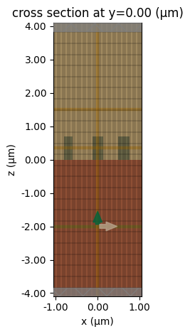
We build the notched three-bar supercell and visualize the geometry before running. The simulation is now fully 3D: the supercell is periodic in (x) with period (3p_{\mathrm{bar}}), and periodic in (y) with the notch period (p_{\mathrm{notch}}) derived from the guided-mode analysis. PML boundaries are applied along (z) as before.
w1, w2, w3 = best["w"]

sim_3bar_notched = make_3bar_notched_sim(w1, w2, w3, dl=0.02)

ax = sim_3bar_notched.plot(y=0)
sim_3bar_notched.plot_grid(y=0, ax=ax)
ax.set_aspect(0.8)
plt.show()
sim_3bar_notched_data = web.run(
    sim_3bar_notched,
    task_name="3bar_notched_sim",
    path="data/tutorial/3bar_notched_sim.hdf5",
)
14:25:09 -03 WARNING: Simulation has 2.63e+06 time steps. The 'run_time' may be
             unnecessarily large, unless there are very long-lived resonances.
             Created task '3bar_notched_sim' with resource_id
             'fdve-a69a4df7-3704-4539-9e0f-7373eded2fa5' and task_type 'FDTD'.
             View task using web UI at
             'https://tidy3d.simulation.cloud/workbench?taskId=fdve-a69a4df7-370
             4-4539-9e0f-7373eded2fa5'.
Task folder: 'default'.
Output()
14:25:13 -03 Estimated FlexCredit cost: 1.691. Minimum cost depends on task
             execution details. Use 'web.real_cost(task_id)' to get the billed
             FlexCredit cost after a simulation run.
14:25:15 -03 status = queued
             To cancel the simulation, use 'web.abort(task_id)' or
             'web.delete(task_id)' or abort/delete the task in the web UI.
             Terminating the Python script will not stop the job running on the
             cloud.
Output()
14:25:21 -03 status = preprocess
14:25:27 -03 starting up solver
running solver
Output()
14:27:08 -03 status = postprocess
Output()
14:28:30 -03 status = success
14:28:32 -03 View simulation result at
             'https://tidy3d.simulation.cloud/workbench?taskId=fdve-a69a4df7-370
             4-4539-9e0f-7373eded2fa5'.
Output()
14:30:17 -03 Loading results from data/tutorial/3bar_notched_sim.hdf5
Diffraction Efficiency Spectrum
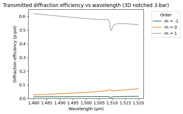
We first examine the transmitted diffraction efficiency as a function of wavelength. Unlike the unperturbed three-bar supercell, which shows a smooth broadband response, the notched structure should exhibit a sharp spectral feature near the guided-mode resonance wavelength. The (m = 1) order — the beam-steered channel — is the most informative one to examine, since the resonance modulates exactly the channel that carries the steered beam.
diff_t = sim_3bar_notched_data["t"]

freqs_3bar = np.asarray(diff_t.f)
lams = td.constants.C_0 / freqs_3bar
lams_um = lams

amps = diff_t.amps
amps_p = amps.sel(polarization="p")
eta_p = np.abs(amps_p) ** 2

try:
    eta_p_1d = eta_p.squeeze("orders_y")
except Exception:
    eta_p_1d = eta_p

orders_x = np.asarray(eta_p_1d.coords["orders_x"])

fig, ax = plt.subplots(figsize=(6, 4))

for m in orders_x:
    eta_m = np.asarray(eta_p_1d.sel(orders_x=m))
    ax.plot(lams_um, eta_m, label=f"m = {m}")

ax.set_xlabel("Wavelength (µm)")
ax.set_ylabel("Diffraction efficiency (p-pol)")
ax.set_title("Transmitted diffraction efficiency vs wavelength (3D notched 3-bar)")
ax.legend(title="Order", bbox_to_anchor=(1.05, 1), loc="upper left")
ax.set_ylim(0, 1.05 * np.max(np.asarray(eta_p_1d)))

fig.tight_layout()
plt.show()
Near-Field Visualization at Resonance
To confirm that the spectral feature is associated with guided-mode excitation, we identify the resonance wavelength from the minimum of the (m = 1) diffraction order and extract the near-field at that frequency. Plotting both (\mathrm{Re}(E_x)) and (|E|) on the (xz) plane provides complementary information: the real part reveals the oscillatory phase structure of the resonantly excited mode, while the field magnitude shows where energy is localized within the bar and surrounding medium.
diff_t = sim_3bar_notched_data["t"]
xz = sim_3bar_notched_data["xz_field"]

# --- find resonance from minimum of transmitted first diffraction order ---
freqs_diff = np.asarray(diff_t.f)
lams_diff = td.C_0 / freqs_diff

amps_p = diff_t.amps.sel(polarization="p")
eta_p = np.abs(amps_p) ** 2

try:
    eta_p = eta_p.squeeze("orders_y")
except Exception:
    pass

eta_m1 = np.asarray(eta_p.sel(orders_x=1))
i_res = np.argmin(eta_m1)

freq_res = freqs_diff[i_res]
lam_res = lams_diff[i_res]

print(f"Resonant wavelength from m=1 minimum: {lam_res:.6f} um")
print(f"Resonant frequency: {freq_res:.6e} Hz")

# --- extract xz-plane fields at the resonant frequency ---
Ex = xz.Ex.sel(f=freq_res, method="nearest").squeeze()
Ey = xz.Ey.sel(f=freq_res, method="nearest").squeeze()
Ez = xz.Ez.sel(f=freq_res, method="nearest").squeeze()

if Ex.dims == ("z", "x"):
    Ex = Ex.transpose("x", "z")
    Ey = Ey.transpose("x", "z")
    Ez = Ez.transpose("x", "z")

x = np.asarray(Ex.coords["x"])
z = np.asarray(Ex.coords["z"])

Ex_np = np.asarray(Ex)
Ey_np = np.asarray(Ey)
Ez_np = np.asarray(Ez)

Ex_real = np.real(Ex_np)
Eabs = np.sqrt(np.abs(Ex_np) ** 2 + np.abs(Ey_np) ** 2 + np.abs(Ez_np) ** 2)

# --- plot side by side ---
fig, axes = plt.subplots(1, 2, figsize=(13, 5), constrained_layout=True)

# Re(Ex), closer to the web interface style
v = np.max(np.abs(Ex_real))
pcm0 = axes[0].pcolormesh(
    x,
    z,
    Ex_real.T,
    shading="auto",
    cmap="RdBu_r",
    vmin=-v,
    vmax=v,
)
axes[0].set_xlabel("x (µm)")
axes[0].set_ylabel("z (µm)")
axes[0].set_title(rf"$\mathrm{{Re}}(E_x)$ at $\lambda \approx {lam_res:.4f}\,\mu$m")
axes[0].set_aspect("equal")
fig.colorbar(pcm0, ax=axes[0], label=r"$\mathrm{Re}(E_x)$ (arb. units)")

# |E|, good for guided-mode visualization
pcm1 = axes[1].pcolormesh(
    x,
    z,
    Eabs.T,
    shading="auto",
    cmap="inferno",
)
axes[1].set_xlabel("x (µm)")
axes[1].set_ylabel("z (µm)")
axes[1].set_title(rf"$|E|$ at $\lambda \approx {lam_res:.4f}\,\mu$m")
axes[1].set_aspect("equal")
fig.colorbar(pcm1, ax=axes[1], label=r"$|E|$ (arb. units)")

plt.show()
Resonant wavelength from m=1 minimum: 1.509637 um
Resonant frequency: 1.985859e+14 Hz
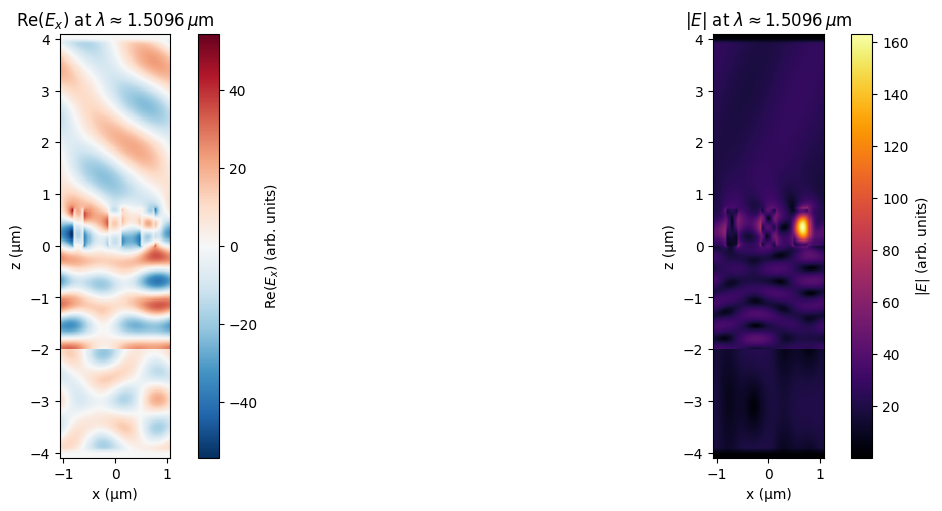
The field plots confirm that the sharp spectral feature arises from resonant excitation of the guided mode identified in the mode-solver analysis. The strong near-field localization within the bar and the structured spatial pattern along (z) are characteristic signatures of a weakly radiative guided-mode resonance.
Together, the diffraction spectrum and near-field maps demonstrate the central result of this tutorial: by combining a phase-gradient supercell with a weak periodic perturbation, it is possible to realize a metasurface that simultaneously steers light into a chosen diffraction order and exhibits a high-(Q) spectral response. This design principle is the basis of the resonant phase-gradient metasurfaces demonstrated experimentally in the cited literature.
Summary
| Design element | Role |
|---|---|
| Bar width sweep | Provides phase library for local phase control |
| Phase-triplet selection | Identifies three widths spanning (2\pi) with high transmission |
| Three-bar supercell | Imposes a linear phase ramp to steer light into the (m = \pm 1) order |
| Guided-mode analysis | Determines the perturbation period needed for resonant coupling |
| Periodic notch | Weakly couples free-space light into the guided mode, producing a high-(Q) resonance |
| Notched supercell | Combines beam steering and high-(Q) spectral selectivity in a single device |