Author: Dominic Thompson, Queen's University
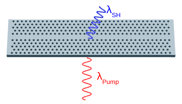
Photonic crystal waveguides (PCWs) offer an exciting platform for enhancing light-matter interactions due to their ability to generate regions of very large group index $n_g>30$. In this notebook, we will demonstrate how to calculate the band structure, modes, and group index for the W1 PCW. We will then use this information to compute the Purcell Enhancement, a quantity that reduces the lifetime and increases the indistinguishability of quantum emitters.
Overview
- Set up the geometry of the W1 PCW.
- Set the source and monitor response times so that we only observe the resonant response of the PCW.
- We use Bloch boundary conditions and the ResonanceFinder plugin to compute the band structure of the PCW.
- Run the band structure simulations again with field monitors targeting the frequencies of the guided Bloch modes in the PCW.
- Use the PCW Bloch modes to calculate the group index through the Hellmann-Feynman Theorem.
- Use the group index and normalized Bloch mode to calculate the Purcell Enhancement.
The Hellmann-Feynman Theorem method for computing group index is covered in the work of John D. Joannopoulos, Steven G. Johnson, Joshua N. Winn, and Robert D. Meade, entitled "Photonic Crystals: Molding the Flow of Light, Second Edition", Princeton University Press, 2008.
The method used to calculate the Purcell Enhancement, along with the geometry benchmarked against, is laid out in V. S. C. Manga Rao and S. Hughes, entitled "Single quantum-dot Purcell factor and β factor in a photonic crystal waveguide", Physical Review B, 2007. DOI: https://doi.org/10.1103/PhysRevB.75.205437
# import relevant libraries
import matplotlib.pyplot as plt
import numpy as np
import tidy3d as td
from tidy3d import web
from tidy3d.plugins.resonance import ResonanceFinder
Geometry Set Up
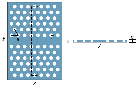
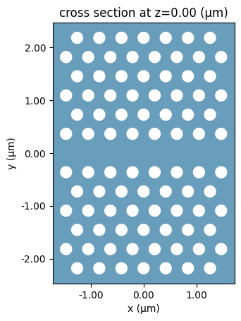
The W1 PCW has the geometry shown above. We will only include a single unit cell in our simulation, shown by the black dashed box, but we define the whole slab for ease of use. There is a buffer added to the width and length of the slab such that holes do not overlap with the edges.
The relevant geometric parameters, materials, and frequency parameters are defined below.
#lattice constant
a = 0.420

#number in each direction
Ny = 13 # Number of rows in the PCW. Should be odd number to account for the center row.
Nx = 8 # Number of unit cells in the x direction
pitch = np.sqrt(3)/2 # Define the pitch of the PCW, set by the hexagonal lattice of the W1

#some basic parameters for the slab
d_thick = 0.5*a # Define the thickness of the slab
hole_radius = 0.275*a # Define the radius of the holes
extra_width = 0.1*a # Define the extra width of the slab
extra_height = 0.25*a # Define the extra height of the slab
slab_length = Nx*a+2*extra_width # Define the length of the slab
slab_width = Ny*a*pitch+2*extra_height # Define the width of the slab

#set up the mins and maxes
freq_min = 180E12
freq_max = 230E12

#set up the frequency range
num_freqs = 151
freqs = np.linspace(freq_min, freq_max, num_freqs)
freq0 = np.mean(freqs)

#set up the width of the frequency range
fwidth = freq0 / 10

#define the run time
run_time = 30 / fwidth

#define the materials
n_slab = np.sqrt(12)
n_clad = 1
slab_Medium = td.Medium(permittivity=n_slab**2)
clad_Medium = td.Medium(permittivity=n_clad**2)
We define the full geometry of the slab with our slab material, and add the holes by adding cylinders of the cladding material.
# define the geometry of the slab
def get_geometry(Nx=Nx,Ny=Ny):

    #define the slab
    slab = td.Structure(geometry=td.Box(center=[0, 0, 0], size=[slab_length, slab_width, d_thick]), medium=slab_Medium)

    # define the holes
    holes_group = []
    for xi in np.arange(Nx)-Nx//2:
        for yi in np.arange(Ny)-Ny//2:
            if yi == 0 or (xi == -Nx//2 and yi%2==0):
                continue
            elif yi%2 == 1:
                center = [a*xi+.5*a, a*yi*pitch, 0]
            else:
                center = [a*xi, a*yi*pitch, 0]
            holes_group.append(td.Cylinder(center=center, radius=hole_radius, length=d_thick))
    holes = td.Structure(geometry=td.GeometryGroup(geometries=holes_group), medium=clad_Medium)


    #define the geometry
    return [slab, holes]
Quickly view the PCW slab using the Scene function
fig, ax = plt.subplots(1,1)
structures = get_geometry(Nx=Nx,Ny=Ny)

scene = td.Scene(
    structures=structures,
    medium=clad_Medium,
)

scene.plot(z=0, ax=ax)

plt.show()
Source and Monitor Times
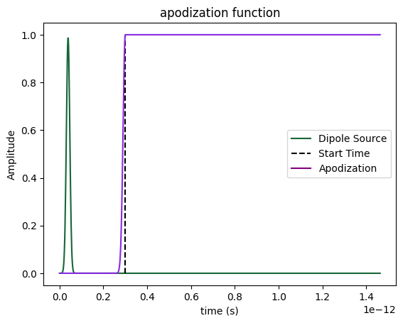
We will be exciting the modes of the PCW using dipole sources and monitoring the response using FieldTimeMonitors and FieldMonitors for finding the resonances and Bloch modes, respectively. For these monitors, we are not interested in the initial dipole source, but rather the resonant response of the PCW. To exclude the dipole source from these computations, we need to ensure that we start monitoring the field well after the dipole source has finished emitting. Below, we plot the dipole source in time along with the start time of the FieldTimeMonitors and the apodization of the FieldMonitor.
# time for apodization to start
source_time = td.GaussianPulse(freq0=freq0, fwidth=fwidth)
t_start = 3e-13
apodization = td.ApodizationSpec(start=t_start, width=10e-15)
# plot the dipole source in time, we can see they turn on well after the source has finished emitting
fig,ax = plt.subplots(1,1)
times = np.linspace(0,run_time,1000)
ax.plot(times,np.abs(source_time.amp_time(times)),label='Dipole Source')
ax.vlines(t_start,0,1,color='black',linestyle='--',label='Start Time')
apodization.plot(times, ax=ax)
ax.plot([], [], color='purple', label='Apodization')  # add a dummy plot just for legend label
ax.set_ylabel('Amplitude')
ax.legend()
plt.show()
Band Structure Simulation
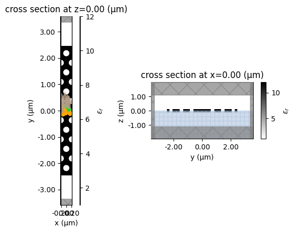
To simulate the band structure of the PCW, we isolate one unit cell of the PCW and add Bloch boundary conditions on the left and right sides of the unit cell. This only allows modes with the specified Bloch vector to remain resonant in the PCW. Therefore, by sweeping the Bloch vector, we can use the ResonanceFinder plugin to calculate the resonant frequencies of the PCW for each Bloch vector. We are only interested in the modes traveling along the waveguide, so we only add Bloch boundary conditions along the x-axis and use PML for the rest.
We excite all of the TE modes in the waveguide by randomly distributing a few y-polarized dipole sources in the center region of the PCW. A few sources are used instead of one to ensure we overlap with all TE modes. Similarly, a few randomly distributed monitors are used to pick up the resonant response, with the time windowing discussed before.
We also allow for the inclusion of the field monitor in the simulation. This will be used later for computing the Bloch mode electric field distribution.
def get_band_sim(Ny=Ny, bloch_vec=0, Nsources=5, Nmonitors=5, include_field_monitor=False, field_monitor_freq=freq0):

    # set the random seed for reproducibility
    np.random.seed(42)

    # get the geometry of the PCW
    structures = get_geometry(Nx=Ny)

    # define the size of the simulation
    sim_size = (
        a,
        a*pitch*Ny+2,
        d_thick+2,
    )

    #add the dipole source in the center of the slab
    sources = []
    for i in range(Nsources):
        xpos_dipole = np.random.uniform(-a/2, a/2)
        ypos_dipole = np.random.uniform(-a*pitch/2, a*pitch/2)
        dipole_center = [xpos_dipole, ypos_dipole, 0]
        dipole_source = td.PointDipole(
            center=dipole_center,
            size=[0,0,0],
            source_time=source_time,
            polarization="Ey",
            name="dipole_source_" + str(i),
        )
        sources.append(dipole_source)

    #add the monitors
    monitors = []
    for i in range(Nmonitors):
        xpos_monitor = np.random.uniform(-a/2, a/2)
        ypos_monitor = np.random.uniform(-a*pitch/2, a*pitch/2)
        monitor_center = [xpos_monitor, ypos_monitor, 0]
        time_monitor = td.FieldTimeMonitor(
            fields=["Ey"],
            center=monitor_center,
            size=(0, 0, 0),
            start=t_start,
            name="monitor_time_" + str(i),
        )
        monitors.append(time_monitor)

    if include_field_monitor:
        field_mnt_size = [sim_size[0], sim_size[1], sim_size[2]]
        field_mnt = td.FieldMonitor(
            center=[0, 0, 0],
            size=field_mnt_size,
            freqs=[field_monitor_freq],
            name="field",
            apodization=apodization,
        )
        monitors.append(field_mnt)

    # make the grid specs, ensure that the grid in x and y line up with the unit cell size
    steps_per_unit_length = 20
    grid_spec = td.GridSpec(
        grid_x=td.UniformGrid(dl=a / steps_per_unit_length),
        grid_y=td.UniformGrid(dl=a / steps_per_unit_length * pitch),
        grid_z=td.AutoGrid(min_steps_per_wvl=steps_per_unit_length),
    )

    # define the boundary conditions, bloch boundary on the x-axis and pml on the y and z-axes
    boundary_spec = td.BoundarySpec(
        x=td.Boundary.bloch(bloch_vec),
        y=td.Boundary.pml(),
        z=td.Boundary.pml(),
    )

    # set up the simulation
    sim = td.Simulation(
        size=sim_size,
        grid_spec=grid_spec,
        structures=structures,
        sources=sources,
        monitors=monitors,
        run_time=run_time,
        boundary_spec=boundary_spec,
        symmetry=(0, 0, 1),
        medium=clad_Medium,
        shutoff=0    # ensure we run for the full simulation time for ResonanceFinder
    )

    return sim
# Show the simulation of the PCW with the sources and monitors
sim = get_band_sim(Ny=Ny, include_field_monitor=False, bloch_vec=0, Nsources=5, Nmonitors=5)
fig,axs = plt.subplots(1,2)
sim.plot_eps(z=0,ax=axs[0])
sim.plot_eps(x=0,ax=axs[1])
plt.show()
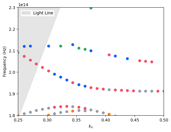
We compute the band structure by using 25 separate $k_x(2\pi/a)$ Bloch vectors ranging from $0.25$ to $0.5$.
Note: Simulations are run locally; this may take several minutes.
ks = np.linspace(0.25,0.5,25) # bloch vectors
sims = {}
for i,k in enumerate(ks):
    sims[f"sim_{i}"] = get_band_sim(Ny=Ny, bloch_vec=k)

# initialize a batch and run them all
batch = web.Batch(simulations=sims, verbose=True)

# run the batch and store all of the data in the `data/` dir.
path = "data/tidy3d_output"
batch_data = batch.run(path_dir=path)
Output()
09:41:33 EDT Started working on Batch containing 25 tasks.
09:41:58 EDT Maximum FlexCredit cost: 0.625 for the whole batch.
             Use 'Batch.real_cost()' to get the billed FlexCredit cost after
             completion.
Output()
09:42:32 EDT Batch complete.
For each simulation, we pull out the resonant frequencies using the ResonanceFinder plugin. This will return all resonances found for the PCW within the frequency range we studied, so we store all resonant frequencies found within "bands." We will then find the band we are interested in and isolate those resonant frequencies.
resonance_finder = ResonanceFinder(freq_window=tuple((freqs[0],freqs[-1])))
bands = np.zeros((len(batch_data.keys()),20)) # for storing all resonant frequencies found

# Loop through each simulation and store the resonances
for i,key in enumerate(batch_data.keys()):
    resonance_data = resonance_finder.run(signals=batch_data[key].data)
    resonance_freqs = resonance_data.freq.to_numpy()
    bands[i,:len(resonance_freqs)] = resonance_freqs
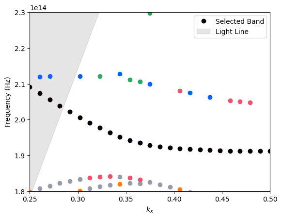
The plot below shows the resonances found for the PCW, with the light line shown as the gray shaded region. The band we are interested in is the one that has a frequency of approximately 190 THz at $k_x=0.5$. As can be seen from the different colors of the points along the band, the indices of the resonances found on this band are not consistent for all $k_x$ values.
plt.plot(ks,bands,'o')
plt.fill_between(ks, 1E15, (ks/n_clad/a*td.C_0), color='gray', alpha=0.2,label='Light Line')
plt.ylim(freqs[0],freqs[-1])
plt.xlim(0.25,0.5)
plt.xlabel(r'$k_x$')
plt.ylabel(r'Frequency (Hz)')
plt.legend()
plt.show()
We isolate the band we are interested in by working backward through the $k_x$ points and adding the frequency that keeps the band continuous.
# band frequency at k_x=0.5
final_band_freq = 190E12
band_interest = np.zeros(len(ks))

# Choose the frequency that keeps the band continuous
for i in range(len(ks)):
    if i == 0:
        band_interest[-1] = bands[-1,np.argmin(np.abs(bands[-1,:]-final_band_freq))]
    else:
        band_interest[-i-1] = bands[-i-1,np.argmin(np.abs(bands[-i-1,:]-band_interest[-i]))]
plt.plot(ks,bands,'o')
plt.plot(ks,band_interest,'o',color='black',label='Selected Band')
plt.fill_between(ks, 1E15, (ks/n_clad/a*td.C_0), color='gray', alpha=0.2,label='Light Line')
plt.ylim(freqs[0],freqs[-1])
plt.xlim(0.25,0.5)
plt.xlabel(r'$k_x$')
plt.ylabel(r'Frequency (Hz)')
plt.legend()
plt.show()
Mode Calculation
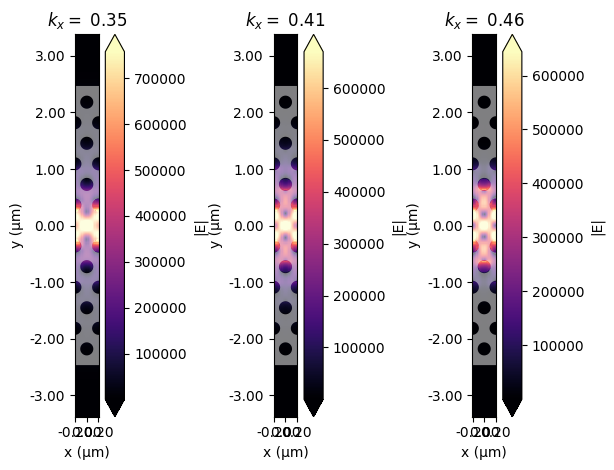
We now know the frequency associated with every Bloch vector we are interested in. Using this, we run a second set of simulations that includes the FieldMonitor and the apodization previously defined for the frequency we just calculated. This will give us the Bloch mode electric field profile for the Bloch vectors used.
Note: Simulations are run locally; this may take several minutes.
sims = {}
for i,k in enumerate(ks):
    sims[f"sim_{i}"] = get_band_sim(Ny=Ny, bloch_vec=k, include_field_monitor=True, field_monitor_freq=band_interest[i])

# initialize a batch and run them all
batch_fields = web.Batch(simulations=sims, verbose=True)

# run the batch and store all of the data in the `data/` dir.
path = "data/tidy3d_output"
batch_data_fields = batch_fields.run(path_dir=path)
Output()
09:43:02 EDT Started working on Batch containing 25 tasks.
09:43:28 EDT Maximum FlexCredit cost: 0.625 for the whole batch.
             Use 'Batch.real_cost()' to get the billed FlexCredit cost after
             completion.
Output()
09:45:00 EDT Batch complete.
fig, axs = plt.subplots(1,3)
batch_data_fields["sim_10"].plot_field("field", "E", val="abs", z=0, eps_alpha=.5, ax=axs[0])
axs[0].set_title(fr'$k_x=$ {ks[10]:.2f}')
batch_data_fields["sim_15"].plot_field("field", "E", val="abs", z=0, eps_alpha=.5, ax=axs[1])
axs[1].set_title(fr'$k_x=$ {ks[15]:.2f}')
batch_data_fields["sim_20"].plot_field("field", "E", val="abs", z=0, eps_alpha=.5, ax=axs[2])
axs[2].set_title(fr'$k_x=$ {ks[20]:.2f}')
plt.tight_layout()
plt.show()
Compute Group Index
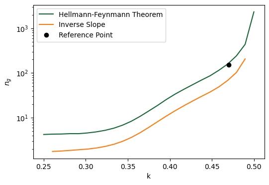
The group index can be computed in two ways
- Through the inverse slope of the band
$$n_g(\omega_k)=c\frac{dk}{d\omega_k}$$
where $\omega$ is the angular frequency
- Through the Hellmann-Feynman Theorem $$n_g(\omega_k) = \frac{2c(U_{e,k} + U_{h,k})}{\left| \int_{V} d\mathbf{r} \, \text{Re}[\mathbf{e}_k^*(\mathbf{r}) \times \mathbf{h}_k(\mathbf{r})] \right|}$$
where $e$ is the electric field Bloch mode, $h$ is the magnetic field Bloch mode, $V$ is the volume of a unit cell, $U_{e}$ and $U_{h}$ are the time-averaged electric and magnetic field energies, and are calculated as
$$U_e = \frac{\varepsilon_0}{4} \int_{V} \varepsilon(\mathbf{r}) |\mathbf{e}_k(\mathbf{r})|^2 \, d\mathbf{r}\\ U_h = \frac{\mu_0}{4} \int_{V} |\mathbf{h}_k(\mathbf{r})|^2 \, d\mathbf{r}$$
We normalize our electric field such that
$$\int_{V} \varepsilon(\mathbf{r}) |\mathbf{e}_k(\mathbf{r})|^2 \, d\mathbf{r}=1 \\ \frac{\mu_0}{\varepsilon_0}\int_{V} |\mathbf{h}_k(\mathbf{r})|^2 \, d\mathbf{r}=1$$
We also know from the virial-like theorem that $U_e=U_h$ for any Bloch mode. Therefore the numerator of the group index computation becomes $2c(U_e+U_h)=c\varepsilon_0$ and therefore $$n_g(\omega_k) = \frac{c\varepsilon_0}{\left| \int_{V} d\mathbf{r} \, \text{Re}[\mathbf{e}_k^*(\mathbf{r}) \times \mathbf{h}_k(\mathbf{r})] \right|}$$
We will show the computation using both methods and find that the Hellmann-Feynman Theorem gives more accurate results since we have limited Bloch vector resolution.
# Compute the norm of the electric and magnetic fields
def calc_norm(sim_data):

    # Pull out the electric field
    Ex = sim_data['field'].Ex.isel(f=0)
    Ey = sim_data['field'].Ey.isel(f=0)
    Ez = sim_data['field'].Ez.isel(f=0)

    # Pull out the permittivity
    box_size = [1, slab_width, d_thick*6]
    full_box = td.Box(center=[0, 0, 0], size=box_size)
    eps = sim_data.simulation.epsilon(box=full_box, coord_key='centers')

    # interpolate the field to the permittivity grid
    Ex_interp = Ex.interp_like(eps,method='linear')
    Ey_interp = Ey.interp_like(eps,method='linear')
    Ez_interp = Ez.interp_like(eps,method='linear')

    # compute the norm
    Enorm = (eps*(np.abs(Ex_interp)**2 + np.abs(Ey_interp)**2 + np.abs(Ez_interp)**2)).integrate(coord=('x','y','z')).item()

    # compute the magnetic field norm
    Hx = sim_data['field'].Hx.isel(f=0)
    Hy = sim_data['field'].Hy.isel(f=0)
    Hz = sim_data['field'].Hz.isel(f=0)

    # compute the magnetic field norm
    Hnorm = td.MU_0/td.EPSILON_0*(np.abs(Hx)**2 + np.abs(Hy)**2 + np.abs(Hz)**2).integrate(coord=('x','y','z')).item()

    return Enorm, Hnorm
We compute the group index using the Hellmann-Feynman Theorem
def calc_ng_HF(sim_data,Enorm=1,Hnorm=1):

    # Pull out the electric field
    Ex = sim_data['field'].Ex.isel(f=0)/np.sqrt(Enorm)
    Ey = sim_data['field'].Ey.isel(f=0)/np.sqrt(Enorm)
    Ez = sim_data['field'].Ez.isel(f=0)/np.sqrt(Enorm)

    # Pull out the magnetic field
    Hx = sim_data['field'].Hx.isel(f=0)/np.sqrt(Hnorm)
    Hy = sim_data['field'].Hy.isel(f=0)/np.sqrt(Hnorm)
    Hz = sim_data['field'].Hz.isel(f=0)/np.sqrt(Hnorm)

    # Put everything on the same grid, use cubic for increased accuracy
    Ey_interp = Ey.interp_like(Ex, method='linear')
    Ez_interp = Ez.interp_like(Ex, method='linear')
    Hx_interp = Hx.interp_like(Ex, method='linear')
    Hy_interp = Hy.interp_like(Ex, method='linear')
    Hz_interp = Hz.interp_like(Ex, method='linear')

    # compute the cross product
    S_x = np.conj(Ey_interp)*Hz_interp-np.conj(Ez_interp)*Hy_interp
    S_y = np.conj(Ez_interp)*Hx_interp-np.conj(Ex)*Hz_interp
    S_z = np.conj(Ex)*Hy_interp-np.conj(Ey_interp)*Hx_interp

    # compute the integral
    S_x = np.real(S_x.integrate(coord=('x','y','z')).item())
    S_y = np.real(S_y.integrate(coord=('x','y','z')).item())
    S_z = np.real(S_z.integrate(coord=('x','y','z')).item())

    S_norm = np.sqrt(S_x**2+S_y**2+S_z**2)

    # compute the group index
    ng = td.C_0*td.EPSILON_0/S_norm

    return ng

ngs = []
for i in range(len(ks)):
    Enorm,Hnorm = calc_norm(batch_data_fields[f"sim_{i}"])
    ng = calc_ng_HF(batch_data_fields[f"sim_{i}"],Enorm,Hnorm)
    ngs.append(ng)
Plot both methods to compare the results. The reference point is taken from the Hughes paper referenced at the start. It is clear that the Hellmann-Feynman Theorem method is much more accurate. This is due to the limited resolution of the Bloch vector computation. If you were to run many more simulations with a finer Bloch vector resolution, the results would converge.
fig,ax = plt.subplots(1,1,figsize=(6,4))
ax.plot(ks,np.array(ngs),label='Hellmann-Feynman Theorem')

# Compute the group index using the inverse slope of the band and central difference
numer = ks[2:] - ks[:-2]
denom = band_interest[2:] - band_interest[:-2]
central_diff_ng = np.abs(numer / denom)
ax.plot(ks[1:-1],central_diff_ng*td.C_0,label='Inverse Slope')

# plot reference point
ax.plot(0.47,154,'o',color='black',label='Reference Point')

ax.set_yscale('log')
ax.set_xlabel('k')
ax.set_ylabel(r'$n_g$')
ax.legend()
plt.show()
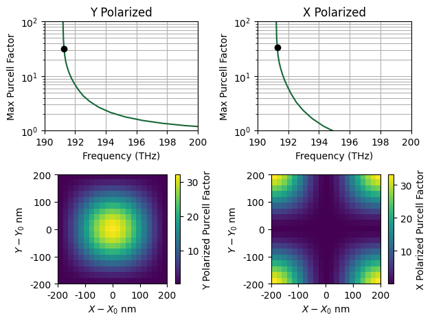
Compute the Purcell enhancement
The Purcell enhancement can be computed using
$$\mathrm{PF}(r_d) = \frac{3\pi c^2 a \left| \mathbf{e}_{k_\omega}(r_d) \cdot \hat{\mathbf{n}} \right|^2n_g(\omega_k)}{\omega_d^2 \sqrt{\varepsilon}}$$
where $r_d$ is the position of the dipole, $\omega_d$ is the frequency of the dipole, $c$ is the speed of light, $\hat{\mathbf{n}}$ is the dipole moment, $\varepsilon$ is the dielectric constant of the slab material, and $\mathbf{e}$ is the normalized electric field bloch mode. We will assume that $\omega_d=\omega_k$.
We only look at the Purcell Factor at the center of the slab $z=0$.
def calc_pf(sim_data,freq=190E12,ng=1,Enorm=1,n=[0,1,0],x_range=(-0.5,0.5),y_range=(-0.5,0.5)):

    # Pull out the electric field within the specified range
    Ex = sim_data['field'].Ex.isel(f=0).sel(x=slice(x_range[0],x_range[1]),y=slice(y_range[0],y_range[1]),z=0)/np.sqrt(Enorm)
    Ey = sim_data['field'].Ey.isel(f=0).sel(x=slice(x_range[0],x_range[1]),y=slice(y_range[0],y_range[1]),z=0)/np.sqrt(Enorm)
    Ez = sim_data['field'].Ez.isel(f=0).sel(x=slice(x_range[0],x_range[1]),y=slice(y_range[0],y_range[1]),z=0)/np.sqrt(Enorm)

    # compute the dot product and coefficient
    dot_prod = np.abs(Ex*n[0]+Ey*n[1]+Ez*n[2])**2
    omega = 2*np.pi*freq
    coef = 3*np.pi*td.C_0**2*a*ng/(omega**2*n_slab)

    return coef*dot_prod
Compute the spatial distributions of the Purcell factor for x and y-polarized dipoles
# compute the purcell enhancement for each simulation
pfs_y = []
pfs_x = []
for i in range(len(ks)):
    Enorm,Hnorm = calc_norm(batch_data_fields["sim_"+str(i)])
    pfs_y.append(calc_pf(batch_data_fields["sim_"+str(i)],freq=band_interest[i],ng=ngs[i],Enorm=Enorm,n=[0,1,0],x_range=(-.2,.2),y_range=(-.2,.2)))
    pfs_x.append(calc_pf(batch_data_fields["sim_"+str(i)],freq=band_interest[i],ng=ngs[i],Enorm=Enorm,n=[1,0,0],x_range=(-.2,.2),y_range=(-.2,.2)))
We pull out the maximum Purcell Factor in the central 400nm by 400nm region of the PCW for both dipoles. We also show the Purcell Factor as a function of position in the central region of the PCW unit cell for both dipoles
k_plot = 21
fig, axs = plt.subplots(2,2)
axs[0,0].plot(band_interest*1E-12,np.max(np.max(pfs_y,axis=1),axis=1))
axs[0,0].plot(band_interest[k_plot]*1E-12,np.max(np.max(pfs_y,axis=1),axis=1)[k_plot],'o',color='black')
axs[0,0].set_xlim(190,200)
axs[0,0].set_ylim(1,1E2)
axs[0,0].set_yscale('log')
axs[0,0].grid(True, which='both', axis='both')
axs[0,0].set_xlabel('Frequency (THz)')
axs[0,0].set_ylabel('Max Purcell Factor')
axs[0,0].set_title('Y Polarized')


axs[0,1].plot(band_interest*1E-12,np.max(np.max(pfs_x,axis=1),axis=1))
axs[0,1].plot(band_interest[k_plot]*1E-12,np.max(np.max(pfs_x,axis=1),axis=1)[k_plot],'o',color='black')
axs[0,1].set_xlim(190,200)
axs[0,1].set_ylim(1,1E2)
axs[0,1].grid(True, which='both', axis='both')
axs[0,1].set_title('X Polarized')
axs[0,1].set_yscale('log')
axs[0,1].set_xlabel('Frequency (THz)')
axs[0,1].set_ylabel('Max Purcell Factor')

# Set extent to the limits of the ticks
x_ticks = [-200, -100, 0, 100, 200]
y_ticks = [-200, -100, 0, 100, 200]
extent = [x_ticks[0], x_ticks[-1], y_ticks[0], y_ticks[-1]]

im = axs[1,0].imshow(pfs_y[k_plot], extent=extent, origin='lower')
axs[1,0].set_xlabel(r'$X-X_0$ nm')
axs[1,0].set_ylabel(r'$Y-Y_0$ nm')
axs[1,0].set_xticks(x_ticks)
axs[1,0].set_yticks(y_ticks)
axs[1,0].set_xticklabels([f"{x}" for x in x_ticks])
axs[1,0].set_yticklabels([f"{y}" for y in y_ticks])
fig.colorbar(im, ax=axs[1,0],label='Y Polarized Purcell Factor')

im = axs[1,1].imshow(pfs_x[k_plot], extent=extent, origin='lower')
axs[1,1].set_xlabel(r'$X-X_0$ nm')
axs[1,1].set_ylabel(r'$Y-Y_0$ nm')
axs[1,1].set_xticks(x_ticks)
axs[1,1].set_yticks(y_ticks)
axs[1,1].set_xticklabels([f"{x}" for x in x_ticks])
axs[1,1].set_yticklabels([f"{y}" for y in y_ticks])
fig.colorbar(im, ax=axs[1,1],label='X Polarized Purcell Factor')


plt.tight_layout()
Conclusion
The band structure, mode profiles, group index, and Purcell factor can all be computed efficiently using Tidy3D and the ResonanceFinder plugin. We hope that this example is useful to the community and encourages more research in PCWs.