





Author: Arvind Saravanakumar, UC Davis
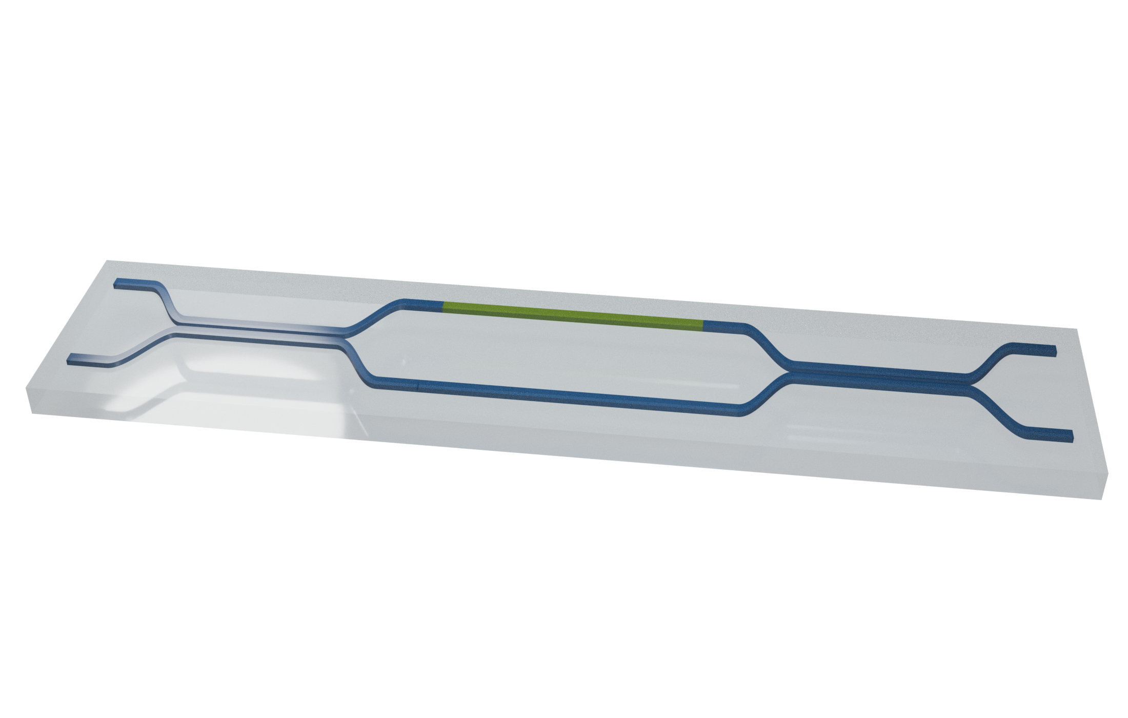
This notebook demonstrates the design and simulation of a tunable silicon photonic Mach-Zehnder interferometer using Tidy3D. The device consists of two directional couplers (3 dB coupling length) connected by two waveguide arms, with one arm containing a phase-shift section. This optimized coupler is then used to construct the MZI, and the phase-section refractive index is swept to demonstrate tunable power transfer between the two output ports.
The notebook highlights how interferometric switching can be modeled using full-wave FDTD simulations and mode monitors. It also connects the device behavior to the 2×2 matrix representation commonly used for programmable photonic circuits.
Simulation Setup
Define the optical wavelength range, waveguide cross section, material indices, and simulation domain. The helper functions in this section assemble the directional couplers, straight waveguide arms, source, and monitors into a reusable MZI model.
import tidy3d as td
import tidy3d.web as web
import numpy as np
import gdstk
import matplotlib.pyplot as plt

# ============================================================
# Parameterized tunable MZI in Tidy3D
# Two directional couplers + one phase-shifted arm
# Units: microns
# ============================================================

# ------------------------------------------------------------
# User parameters
# ------------------------------------------------------------

# Wavelength settings
lambda0 = 1.55
lambda_min = 1.50
lambda_max = 1.60
num_freqs = 10

freq0 = td.C_0 / lambda0
freqs = td.C_0 / np.linspace(lambda_min, lambda_max, num_freqs)

# Waveguide geometry
wg_width = 0.45  # um, y direction
wg_thickness = 0.22  # um, z direction

# Coupler geometry
wg_spacing_in = 5.0  # um, center-to-center spacing of separated arms
wg_spacing_coup = 0.20  # um, edge-to-edge gap in coupling region
wg_length = 3.0  # um, straight input/output length in each coupler
coup_length = 12.18  # um, 3 dB coupling length found from Tidy3D
bend_length = 4.0  # um, cosine S-bend length
sidewall_angle = 0.0

# MZI geometry
phase_length = 20.0  # um, straight phase-shifter section between couplers
phase_arm = "top"  # "top" or "bottom"

# Material indices for simple lossless simulation
n_sio2 = 1.44
n_si = 3.48
phase_index = 3.52  # use 3.48 for passive MZI, larger for phase shift

# Simulation settings
sim_y_span = 8.0
sim_z_span = 3.0
sim_x_padding = 8.0
runtime = 8e-12

# Source/monitor settings
num_modes = 4
mode_plane_y = 2.0
mode_plane_z = 1.5

# Total length of one directional coupler object
dc_total_length = 2 * wg_length + 2 * bend_length + coup_length

# Center the two couplers around x = 0
dc_spacing = dc_total_length + phase_length
dc1_x = -dc_spacing / 2
dc2_x = +dc_spacing / 2
arm_x = 0.0
top_y = +wg_spacing_in / 2
bottom_y = -wg_spacing_in / 2

mzi_x_min = dc1_x - dc_total_length / 2
mzi_x_max = dc2_x + dc_total_length / 2
mzi_length = mzi_x_max - mzi_x_min

# Source and monitor positions
source_x = mzi_x_min + 0.5
monitor_x = mzi_x_max - 0.5

# ------------------------------------------------------------
# Materials
# ------------------------------------------------------------

sio2 = td.Medium(
    name="SiO2_lossless",
    permittivity=n_sio2**2,
)
si = td.Medium(
    name="Si_lossless",
    permittivity=n_si**2,
)

# ------------------------------------------------------------
# Mode specification
# ------------------------------------------------------------

mode_spec = td.ModeSpec(
    num_modes=num_modes,
    sort_spec={
        "filter_reference": 0,
        "filter_order": "over",
        "sort_key": "n_eff",
        "track_freq": "central",
        "keep_modes": "all",
    },
    group_index_step=True,
)


# ------------------------------------------------------------
# Directional coupler structure generator
# ------------------------------------------------------------


def make_directional_coupler(x0, name):
    """
    Creates one symmetric directional coupler centered at x = x0.

    The coupler contains:
    separated input arms -> cosine S-bend -> parallel coupling region
    -> cosine S-bend -> separated output arms.
    """

    cell = gdstk.Cell(name)

    # Top path starts on the upper separated arm.
    x_start = -wg_length - bend_length - coup_length / 2 + x0
    y_start = wg_spacing_in / 2

    top_path = gdstk.RobustPath(
        (x_start, y_start),
        wg_width,
        layer=1,
        datatype=0,
    )

    # Left straight section
    top_path.segment((-bend_length - coup_length / 2 + x0, y_start))

    # The center-to-center spacing in coupling region is:
    # wg_width + wg_spacing_coup
    A = (wg_spacing_in - wg_spacing_coup - wg_width) / 4

    # Bend into coupling region
    top_path.segment(
        (-coup_length / 2 + x0, y_start),
        offset=lambda u: A * np.cos(np.pi * u) - A,
    )

    # Parallel coupling region
    top_path.segment((coup_length / 2 + x0, y_start))

    # Bend out of coupling region
    top_path.segment(
        (bend_length + coup_length / 2 + x0, y_start),
        offset=lambda u: -A * np.cos(np.pi * u) - A,
    )

    # Right straight section
    top_path.segment((wg_length + bend_length + coup_length / 2 + x0, y_start))

    cell.add(top_path)

    # Bottom path is mirrored across y = 0.
    bottom_path = top_path.copy().mirror((0, 0), (1, 0))
    cell.add(bottom_path)

    # Convert GDS paths into a 3D Tidy3D PolySlab.
    dc_geo = td.PolySlab.from_gds(
        cell,
        gds_layer=1,
        axis=2,
        slab_bounds=(-wg_thickness / 2, wg_thickness / 2),
        sidewall_angle=sidewall_angle,
    )

    return td.Structure(
        geometry=td.GeometryGroup(geometries=dc_geo),
        medium=si,
        name=name,
    )


# ------------------------------------------------------------
# Straight arm generator
# ------------------------------------------------------------


def make_straight_arm(x_center, y_center, medium, name):
    """
    Creates a straight waveguide section between the two couplers.
    """

    return td.Structure(
        geometry=td.Box(
            center=(x_center, y_center, 0),
            size=(phase_length, wg_width, wg_thickness),
        ),
        medium=medium,
        name=name,
    )


# ------------------------------------------------------------
# Simulation generator
# ------------------------------------------------------------


def make_mzi_sim(phase_index_value):
    """
    Builds one tunable MZI simulation for a given phase-section material index.
    """
    phase_medium = td.Medium(
        name=f"phase_shift_medium_n_{phase_index_value:.4f}",
        permittivity=phase_index_value**2,
    )

    # Build couplers
    dc1 = make_directional_coupler(dc1_x, "directional_coupler_1")
    dc2 = make_directional_coupler(dc2_x, "directional_coupler_2")

    # Choose which arm is phase shifted
    if phase_arm.lower() == "top":
        top_medium = phase_medium
        bottom_medium = si
        top_name = "top_phase_shifter"
        bottom_name = "bottom_connector"

    elif phase_arm.lower() == "bottom":
        top_medium = si
        bottom_medium = phase_medium
        top_name = "top_connector"
        bottom_name = "bottom_phase_shifter"

    else:
        raise ValueError("phase_arm must be either 'top' or 'bottom'.")

    top_arm = make_straight_arm(
        x_center=arm_x,
        y_center=top_y,
        medium=top_medium,
        name=top_name,
    )
    bottom_arm = make_straight_arm(
        x_center=arm_x,
        y_center=bottom_y,
        medium=bottom_medium,
        name=bottom_name,
    )
    waveguides = [
        make_straight_arm(
            x_center=(dc_total_length + phase_length) * sign,
            y_center=y,
            medium=si,
            name=f"waveguide_{ii}_{jj}",
        )
        for ii, y in enumerate([top_y, bottom_y])
        for jj, sign in enumerate([-1, 1])
    ]

    structures = [dc1, dc2, top_arm, bottom_arm] + waveguides

    source = td.ModeSource(
        name="input_mode_source",
        center=(source_x, bottom_y, 0),
        size=(0, mode_plane_y, mode_plane_z),
        source_time=td.GaussianPulse(
            freq0=freq0,
            fwidth=freq0 / 10,
        ),
        direction="+",
        mode_spec=mode_spec,
    )

    top_monitor = td.ModeMonitor(
        name="top_output_mode_monitor",
        center=(monitor_x, top_y, 0),
        size=(0, mode_plane_y, mode_plane_z),
        freqs=freqs,
        mode_spec=mode_spec,
    )
    bottom_monitor = td.ModeMonitor(
        name="bottom_output_mode_monitor",
        center=(monitor_x, bottom_y, 0),
        size=(0, mode_plane_y, mode_plane_z),
        freqs=freqs,
        mode_spec=mode_spec,
    )
    field_monitor = td.FieldMonitor(
        name="field_xy",
        center=(0, 0, 0),
        size=(mzi_length, sim_y_span - 1.0, 0),
        freqs=[freq0],
        fields=["Ex", "Ey", "Ez"],
    )

    sim = td.Simulation(
        center=(0, 0, 0),
        size=(mzi_length + sim_x_padding, sim_y_span, sim_z_span),
        grid_spec=td.GridSpec.auto(wavelength=lambda0),
        run_time=runtime,
        medium=sio2,
        structures=structures,
        sources=[source],
        monitors=[top_monitor, bottom_monitor, field_monitor],
    )
    return sim


print("MZI geometry summary")
print("--------------------")
print(f"Coupler total length: {dc_total_length:.3f} um")
print(f"Coupler 1 center x:   {dc1_x:.3f} um")
print(f"Coupler 2 center x:   {dc2_x:.3f} um")
print(f"MZI x min:            {mzi_x_min:.3f} um")
print(f"MZI x max:            {mzi_x_max:.3f} um")
print(f"MZI total length:     {mzi_length:.3f} um")

print()
print("Simulation domain")
print("-----------------")
print(f"x span: {mzi_length + sim_x_padding:.3f} um")
print(f"y span: {sim_y_span:.3f} um")
print(f"z span: {sim_z_span:.3f} um")
print(f"source x:  {source_x:.3f} um")
print(f"monitor x: {monitor_x:.3f} um")
MZI geometry summary
--------------------
Coupler total length: 26.180 um
Coupler 1 center x:   -23.090 um
Coupler 2 center x:   23.090 um
MZI x min:            -36.180 um
MZI x max:            36.180 um
MZI total length:     72.360 um

Simulation domain
-----------------
x span: 80.360 um
y span: 8.000 um
z span: 3.000 um
source x:  -35.680 um
monitor x: 35.680 um
Geometry Preview
Plot the baseline device layout before launching the sweep. This check confirms the couplers, arms, phase-shifting section, source, and output monitors are positioned as expected.
sim_base = make_mzi_sim(phase_index_value=phase_index)

fig, ax = plt.subplots(figsize=(12, 4))
sim_base.plot(z=0, ax=ax)
ax.set_title("Parameterized tunable MZI geometry, x-y slice")
plt.tight_layout()
plt.show()

The post-processing helpers extract the quantities used to compare devices across the sweep. get_mode_power returns the forward-propagating TE0 modal power at the selected wavelength, and approximate_phase_shift_rad estimates the accumulated phase shift from the phase-section index change.
def get_mode_power(sim_data, monitor_name, wavelength=1.55, mode_index=0):
    """
    Returns |a|^2 for a selected mode at the chosen wavelength.
    """

    freq = td.C_0 / wavelength
    amps = sim_data[monitor_name].amps

    # Select string/integer coordinates exactly first
    selected = amps.sel(
        direction="+",
        mode_index=mode_index,
    )

    # Select nearest numeric frequency separately
    amp_at_freq = selected.sel(
        f=freq,
        method="nearest",
    )
    return float(np.abs(amp_at_freq.values) ** 2)


def approximate_phase_shift_rad(
    phase_index_value,
    base_index=3.48,
    phase_length_um=20.0,
    wavelength_um=1.55,
    effective_index_sensitivity=0.7,
):
    """
    Approximate MZI phase shift in radians.

    effective_index_sensitivity approximates dneff/dncore.
    It is not exact. For a silicon strip waveguide, values around 0.5–0.8
    are reasonable for a first estimate.
    """
    delta_n_material = phase_index_value - base_index
    delta_n_eff_approx = effective_index_sensitivity * delta_n_material
    delta_phi = 2 * np.pi * delta_n_eff_approx * phase_length_um / wavelength_um
    return delta_phi
Run Batch Simulations
Sweep the phase-section material index and submit the resulting simulations as a Tidy3D batch. Each simulation uses the same geometry and monitors, with only the phase-section index updated.
import pathlib

pathlib.Path("data").mkdir(exist_ok=True)

phase_index_values = np.array(
    [
        3.510,
        3.515,
        3.520,
        3.525,
        3.530,
    ]
)

# Build all simulations up front
sims_dict = {
    f"mzi_phase_index_{str(n).replace('.', 'p')}": make_mzi_sim(n)
    for n in phase_index_values
}

# Submit and run all in parallel
batch_data = web.run_async(
    simulations=sims_dict,
    path_dir="./data",
    verbose=True,
)
Output()
14:45:35 KST Started working on Batch containing 5 tasks.
14:45:42 KST Maximum FlexCredit cost: 3.123 for the whole batch.
             Use 'Batch.real_cost()' to get the billed FlexCredit cost after
             completion.
Output()
14:47:45 KST Batch complete.
Results and Analysis
Switching Condition for a Balanced MZI
For an ideal balanced Mach-Zehnder interferometer built from two identical 3 dB directional couplers, the output state is determined by the relative phase difference between the two arms. Up to a port-dependent phase convention, the normalized output powers can be written as
$$ P_1 = \cos^2\left(\frac{\Delta \phi}{2}\right), \qquad P_2 = \sin^2\left(\frac{\Delta \phi}{2}\right). $$
Therefore, when the arms have no relative phase shift,
$$ \Delta \phi = 0, $$
the output is ideally
$$ (P_1, P_2) = (1, 0). $$
When the relative phase shift reaches
$$ \Delta \phi = \pi, $$
the interference condition is reversed and the output switches to
$$ (P_1, P_2) = (0, 1). $$
More generally, one output state occurs when
$$ \Delta \phi = 2m\pi, $$
and the switched state occurs when
$$ \Delta \phi = (2m+1)\pi, $$
where (m) is an integer.
The phase shift introduced by changing the effective index of one arm is approximately
$$ \Delta \phi = \frac{2\pi}{\lambda_0} \Delta n_\mathrm{eff} L_\mathrm{phase}. $$
For a full switch, we set $\Delta \phi = \pi$. Therefore,
$$ \pi = \frac{2\pi}{\lambda_0} \Delta n_\mathrm{eff} L_\mathrm{phase}. $$
Solving for the required effective-index change gives
$$ \Delta n_\mathrm{eff} = \frac{\lambda_0}{2L_\mathrm{phase}}. $$
For this design, $\lambda_0 = 1.55~\mu\mathrm{m}$ and $L_\mathrm{phase} = 20~\mu\mathrm{m}$, so
$$ \Delta n_\mathrm{eff} = \frac{1.55}{2(20)} \approx 0.03875. $$
Thus, the phase-shifted arm should have an effective index approximately (0.039) larger than the unperturbed arm to produce a full $\pi$-phase shift.
Matrix Form of the MZI Transfer Function
The same switching behavior can also be written in matrix form. This is useful because photonic circuits act on complex optical field amplitudes, not just optical powers. An ideal 3 dB directional coupler can be represented as
$$ C = \frac{1}{\sqrt{2}} \begin{bmatrix} 1 & i \\ i & 1 \end{bmatrix} $$
A phase shifter in one arm can be represented as
$$ P(\Delta \phi) = \begin{bmatrix} 1 & 0 \\ 0 & e^{i\Delta \phi} \end{bmatrix} $$
For an ideal MZI made from two identical 3 dB couplers, the field transfer matrix is
$$ U_\mathrm{MZI}(\Delta \phi) = C P(\Delta \phi) C $$
Substituting the matrices gives
$$ U_\mathrm{MZI}(\Delta \phi) = \frac{1}{2} \begin{bmatrix} 1 - e^{i\Delta \phi} & i\left(1 + e^{i\Delta \phi}\right) \\ i\left(1 + e^{i\Delta \phi}\right) & -1 + e^{i\Delta \phi} \end{bmatrix} $$
This matrix maps the input field amplitudes to the output field amplitudes:
$$ \begin{bmatrix} E_{\mathrm{top,out}} \\ E_{\mathrm{bottom,out}} \end{bmatrix} = U_\mathrm{MZI} \begin{bmatrix} E_{\mathrm{top,in}} \\ E_{\mathrm{bottom,in}} \end{bmatrix}. $$
The measurable output powers are obtained from the squared magnitude of the complex field amplitudes. For example, if light is injected into only one input port, the ideal normalized output powers vary as
$$ P_1 = \cos^2\left(\frac{\Delta \phi}{2}\right), \qquad P_2 = \sin^2\left(\frac{\Delta \phi}{2}\right), $$
depending on the output-port labeling convention. Therefore, changing the phase shift by approximately $\pi$ switches the MZI between its two routing states.
# Ideal 2x2 MZI matrix calculation
def ideal_mzi_matrix(delta_phi):
    """Return the ideal 2x2 MZI field transfer matrix for a phase shift delta_phi."""
    C = (1 / np.sqrt(2)) * np.array(
        [
            [1, 1j],
            [1j, 1],
        ],
        dtype=complex,
    )

    P = np.array(
        [
            [1, 0],
            [0, np.exp(1j * delta_phi)],
        ],
        dtype=complex,
    )
    return C @ P @ C


U_0 = ideal_mzi_matrix(0)
U_pi = ideal_mzi_matrix(np.pi)

print("Ideal MZI field matrix for Δφ = 0:")
print(np.round(U_0, 3))

print("\nPower transfer matrix |U|² for Δφ = 0:")
print(np.round(np.abs(U_0) ** 2, 3))

print("\nIdeal MZI field matrix for Δφ = π:")
print(np.round(U_pi, 3))

print("\nPower transfer matrix |U|² for Δφ = π:")
print(np.round(np.abs(U_pi) ** 2, 3))
Ideal MZI field matrix for Δφ = 0:
[[0.+0.j 0.+1.j]
 [0.+1.j 0.+0.j]]

Power transfer matrix |U|² for Δφ = 0:
[[0. 1.]
 [1. 0.]]

Ideal MZI field matrix for Δφ = π:
[[ 1.-0.j -0.+0.j]
 [-0.+0.j -1.+0.j]]

Power transfer matrix |U|² for Δφ = π:
[[1. 0.]
 [0. 1.]]
Relevance to Photonic Computation
The matrix representation is also why the MZI is a fundamental building block for programmable photonic circuits. In linear optics, the optical field amplitudes at the outputs are linear combinations of the input field amplitudes. Therefore, an MZI implements a tunable $2\times2$ linear transformation.
By adjusting the phase shift, the same physical device can be programmed to route power between ports or to implement intermediate splitting ratios. Larger photonic processors can be built by cascading many tunable MZI blocks into an interferometer mesh. In that setting, each MZI acts as a programmable matrix element, and the full mesh implements a larger matrix-vector multiplication on optical signals. This is the basic connection between tunable interferometers and photonic computing: computation is performed through controlled interference and linear optical transformations.
# Analytical estimate for the effective-index change needed for a full MZI switch
lambda0_est = lambda0
phase_length_est = phase_length
neff_phase_example = 2.35  # example guided-mode effective index near the switched state

required_delta_neff_pi = lambda0_est / (2 * phase_length_est)
neff_base_implied = neff_phase_example - required_delta_neff_pi

print(f"Required Δneff for π phase shift: {required_delta_neff_pi:.5f}")
print(
    f"If neff_phase ≈ {neff_phase_example:.3f}, implied neff_base ≈ {neff_base_implied:.5f}"
)
Required Δneff for π phase shift: 0.03875
If neff_phase ≈ 2.350, implied neff_base ≈ 2.31125
# Extract results from BatchData
results = []

for name, n_phase in zip(sims_dict.keys(), phase_index_values):
    sim_data = batch_data[name]

    p_top = get_mode_power(
        sim_data, "top_output_mode_monitor", wavelength=lambda0, mode_index=0
    )
    p_bottom = get_mode_power(
        sim_data, "bottom_output_mode_monitor", wavelength=lambda0, mode_index=0
    )

    p_sum = p_top + p_bottom
    top_frac = p_top / p_sum if p_sum > 0 else np.nan
    bottom_frac = p_bottom / p_sum if p_sum > 0 else np.nan
    phase_rad = approximate_phase_shift_rad(
        phase_index_value=n_phase,
        base_index=n_si,
        phase_length_um=phase_length,
        wavelength_um=lambda0,
        effective_index_sensitivity=0.7,
    )
    phase_pi = phase_rad / np.pi
    results.append(
        {
            "phase_index": n_phase,
            "p_top": p_top,
            "p_bottom": p_bottom,
            "top_frac": top_frac,
            "bottom_frac": bottom_frac,
            "phase_rad": phase_rad,
            "phase_pi": phase_pi,
        }
    )
    print(
        f"phase_index={n_phase:.4f} | top={top_frac:.4f} | bottom={bottom_frac:.4f} | Δφ={phase_rad:.3f} rad = {phase_pi:.3f}π"
    )
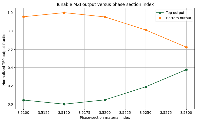
phase_index=3.5100 | top=0.0451 | bottom=0.9549 | Δφ=1.703 rad = 0.542π
phase_index=3.5150 | top=0.0001 | bottom=0.9999 | Δφ=1.986 rad = 0.632π
phase_index=3.5200 | top=0.0470 | bottom=0.9530 | Δφ=2.270 rad = 0.723π
phase_index=3.5250 | top=0.1894 | bottom=0.8106 | Δφ=2.554 rad = 0.813π
phase_index=3.5300 | top=0.3775 | bottom=0.6225 | Δφ=2.838 rad = 0.903π
Collect the batch results into NumPy arrays for plotting. The arrays keep the phase-section indices, normalized output fractions, and estimated phase shifts aligned point by point.
phase_indices = np.array([r["phase_index"] for r in results])
top_fracs = np.array([r["top_frac"] for r in results])
bottom_fracs = np.array([r["bottom_frac"] for r in results])
The final plot compares the normalized TE0 power at the two output ports. As the phase-section index changes, the MZI interference condition shifts and power transfers between the top and bottom outputs.
plt.figure(figsize=(8, 5))
plt.plot(phase_indices, top_fracs, "o-", label="Top output")
plt.plot(phase_indices, bottom_fracs, "o-", label="Bottom output")
plt.xlabel("Phase-section material index")
plt.ylabel("Normalized TE0 output fraction")
plt.title("Tunable MZI output versus phase-section index")
plt.grid(True)
plt.legend()
plt.tight_layout()
plt.show()
Comparison Between Analytical Switching Condition and Simulated Effective Index
For an ideal balanced MZI, full switching occurs when the relative phase shift between the two arms reaches approximately $\pi$. The required effective-index change is
$$ \Delta n_\mathrm{eff} = \frac{\lambda_0}{2L_\mathrm{phase}}. $$
For this design, $\lambda_0 = 1.55~\mu\mathrm{m}$ and $L_\mathrm{phase} = 20~\mu\mathrm{m}$, giving
$$ \Delta n_\mathrm{eff} = \frac{1.55}{2(20)} \approx 0.03875. $$
A separate mode calculation gave an effective index of approximately
$$ n_{\mathrm{eff,base}} \approx 2.35 $$
for the unmodified waveguide and
$$ n_{\mathrm{eff,phase}} \approx 2.39 $$
for the phase-shifted waveguide. Therefore, the simulated effective-index change is
$$ \Delta n_\mathrm{eff} = 2.39 - 2.35 = 0.04. $$
The corresponding phase shift is
$$ \Delta \phi = \frac{2\pi}{1.55}(0.04)(20) \approx 3.24~\mathrm{rad} \approx 1.03\pi. $$
This agrees closely with the analytical switching condition. The FDTD sweep showed nearly complete transfer to the opposite output port near this phase-shifter setting, consistent with the expected $\pi$-phase shift required to switch a balanced MZI from one output state to the other.
Note on Phase-Axis Calibration
It should also be noted that the calibrated phase axis used in the sweep is approximate. In the initial estimate, the material-index change in the phase-shifter section was converted to an effective-index change using an assumed sensitivity factor,
$$ \Delta n_\mathrm{eff} \approx 0.7\Delta n_\mathrm{material}. $$
This factor is only a rough approximation. The true relationship between material index and effective index depends on the waveguide geometry, modal confinement, wavelength, polarization, and surrounding cladding. Since the optical mode is not entirely confined to the silicon core, the effective-index change is smaller than the applied material-index change, but the exact scaling factor should not be assumed universally.
The most accurate way to determine the phase shift is to directly compute the guided-mode effective index for both the unmodified waveguide and the phase-shifted waveguide. The phase difference can then be calculated from
$$ \Delta \phi = \frac{2\pi}{\lambda_0} \left( n_{\mathrm{eff,phase}} - n_{\mathrm{eff,base}} \right) L_\mathrm{phase}. $$
Using separately simulated effective indices, $n_{\mathrm{eff,base}}\approx 2.35$ and $n_{\mathrm{eff,phase}}\approx 2.39$, gives
$$ \Delta n_\mathrm{eff} \approx 0.04, $$
which corresponds to
$$ \Delta \phi = \frac{2\pi}{1.55}(0.04)(20) \approx 3.24~\mathrm{rad} \approx 1.03\pi. $$
This direct effective-index calculation agrees closely with the ideal $\pi$-phase switching condition and is more reliable than the approximate $0.7\Delta n_\mathrm{material}$ estimate.


 TERMS & CONDITIONS


 How the process works:
 Try this real URL to see an example: