





Author: Oliver Liu Wang, Columbia University
The purpose of this notebook is to determine the coupling rate between the fundamental mode of a single-mode waveguide and a phase-matched higher-order mode in an adjacent multimode waveguide. The calculation is done based on coupled mode theory.
Reference: N. V. Vitanov and B. M. Garraway, "Landau-Zener model: Effects of finite coupling duration," Phys. Rev. A 53, 4288 (1996) DOI:10.1103/PhysRevA.53.4288.
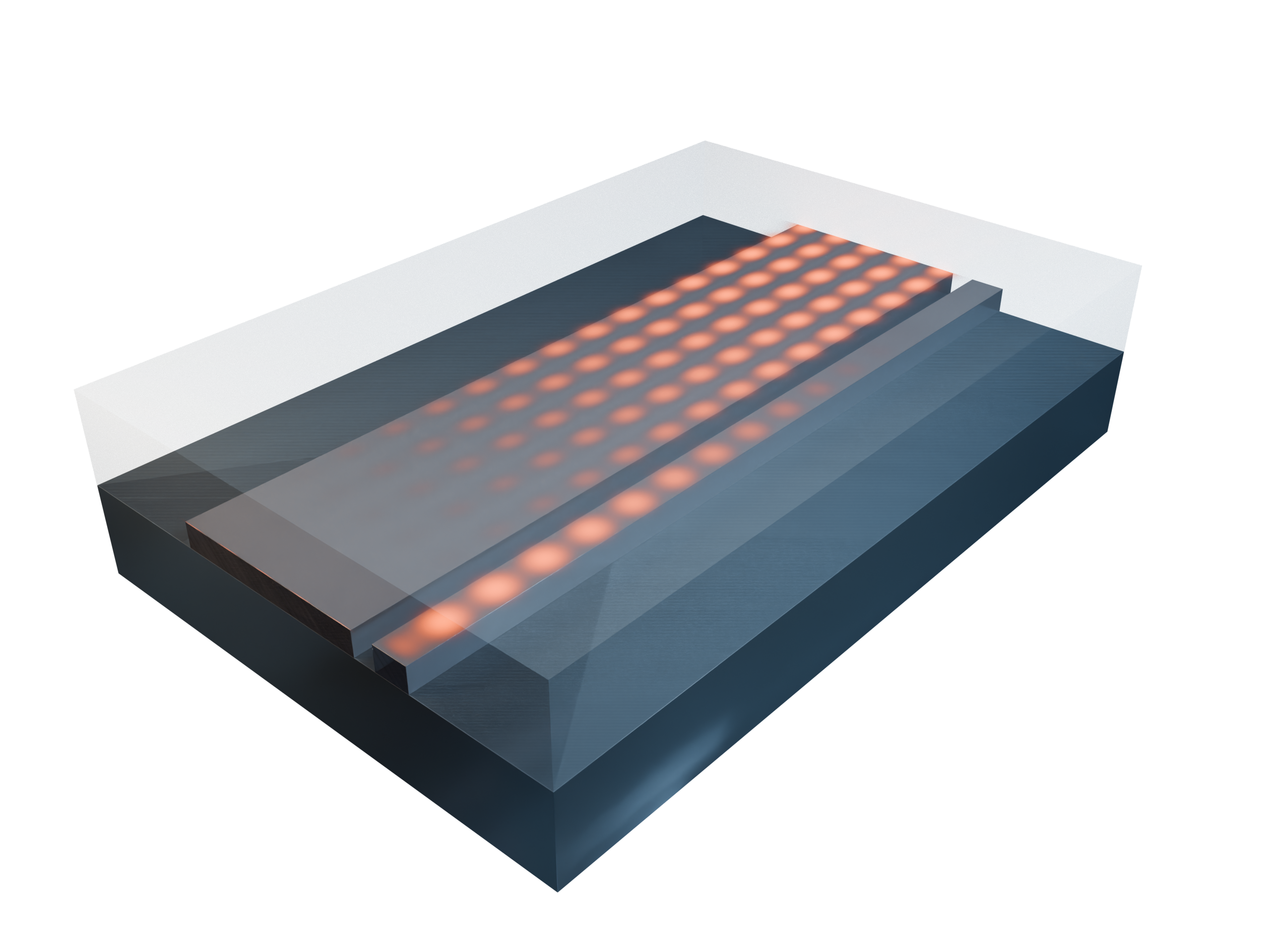
Coupled Mode Theory
In coupled mode theory (Vitanov et al.), the amplitudes of the individual waveguide modes $a_{1,2}$ obey the equation $$ i\frac{d}{dz}\begin{pmatrix} a_1 \\ a_2 \end{pmatrix} = \begin{pmatrix} \Delta(z) & \Omega(z) \\ \Omega(z) & -\Delta(z) \end{pmatrix}\begin{pmatrix} a_1 \\ a_2 \end{pmatrix}\tag{1} $$
Here $z$ is the coordinate along the direction of propagation, $\Delta$ is the propagation constant detuning of each mode from the average propagation constant, $\Omega$ is the coupling rate between the modes, and $i$ is the imaginary unit. We can transform the equation into the basis of supermodes ($c_{1,2}$) instead of individual waveguide modes ($a_{1,2}$) using the following transformation:
$$ \begin{pmatrix} c_1 \\ c_2 \end{pmatrix} = \begin{pmatrix} \cos\left(\vartheta(z)\right) & -\sin\left(\vartheta(z)\right) \\ \sin\left(\vartheta(z)\right) & \cos\left(\vartheta(z)\right) \end{pmatrix}\begin{pmatrix} a_1 \\ a_2 \end{pmatrix} \tag{2} $$ where $\vartheta$ is defined by $$ \tan\left(2\vartheta(z)\right) = \frac{\Omega(z)}{\Delta(z)}\tag{3} $$ In this basis, Eq. (1) becomes $$ i\frac{d}{dz}\begin{pmatrix} c_1 \\ c_2 \end{pmatrix} = \begin{pmatrix} \sqrt{\Delta^2+\Omega^2} & i\frac{d}{dz}\vartheta \\ i\frac{d}{dz}\vartheta & -\sqrt{\Delta^2+\Omega^2} \end{pmatrix}\begin{pmatrix} c_1 \\ c_2 \end{pmatrix}\tag{4} $$
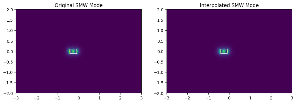
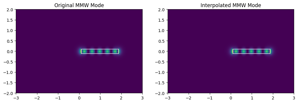
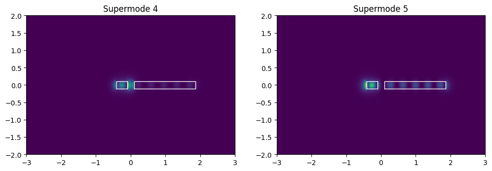
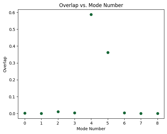
From Eq. (4), it can be seen that the propagation constant detuning for each supermode is $\Delta_s\equiv \pm \sqrt{\Delta^2 + \Omega^2}$. From here, the coupling between the individual waveguide modes can be calculated by $$ \Omega=\sqrt{\left(k_0 n_{eff,avg}-\Delta_s\right)^2 - \Delta^2}\tag{5} $$ Here $k_0 n_{eff,avg}$ is the average propagation constant of the individual waveguide modes being coupled. This code automatically finds the mode in the multimode waveguide that is closest in effective index to the fundamental mode in the single-mode waveguide, and then finds the supermodes based on those two modes when both waveguides are present.
import tempfile

import matplotlib.pyplot as plt
import numpy as np
import tidy3d as td
from scipy.integrate import simpson
from scipy.interpolate import RegularGridInterpolator
from tidy3d import web

td.config.logging.level = "ERROR"
td.config.web.enable_caching = False
td.config.local_cache.enabled = False
Helper Functions
makesim
This function is used for generating the mode data for one particular set of single-mode waveguide width, multimode waveguide width, and gap. The parameters for this function are as follows:
| Variable | Description |
|---|---|
sm_width |
single-mode waveguide width |
core_thickness |
waveguide core layer thickness |
mm_width |
multimode waveguide width |
gap |
edge-to-edge gap between the two waveguides |
smon |
if True, includes the single-mode waveguide in the simulation |
mmon |
if True, includes the multimode waveguide in the simulation |
modenum |
number of modes for the mode solver |
claddingargs |
list containing the type and name of the cladding material to be used from Tidy3D's material library |
coreargs |
list containing the type and name of the core material to be used from Tidy3D's material library |
overridex |
mesh override size in the x (horizontal transverse) direction |
overridey |
mesh override size in the y (vertical transverse) direction |
wavelength |
wavelength used for the mode simulations |
def makesim(
    sm_width=1,
    core_thickness=0.22,
    mm_width=1,
    gap=1,
    smon=True,
    mmon=True,
    modenum=10,
    claddingargs=None,
    coreargs=None,
    overridex=0.01,
    overridey=0.01,
    wavelength=1.55,
):

    if coreargs is None:
        coreargs = ["cSi", "Palik_Lossless"]
    if claddingargs is None:
        claddingargs = ["SiO2", "Palik_Lossless"]
    SiO2 = td.material_library[claddingargs[0]][claddingargs[1]]
    Si = td.material_library[coreargs[0]][coreargs[1]]
    sm = td.Structure(
        geometry=td.Box(
            center=[0, -gap / 2 - sm_width / 2, 0],
            size=[td.inf, sm_width, core_thickness],
        ),
        name="sm",
        medium=Si,
    )

    mm = td.Structure(
        geometry=td.Box(
            center=[0, gap / 2 + mm_width / 2, 0],
            size=[td.inf, mm_width, core_thickness],
        ),
        name="mm",
        medium=Si,
    )

    sm_mesh = td.MeshOverrideStructure(
        name="sm_mesh",
        geometry=td.Box(
            center=[0, -gap / 2 - sm_width / 2, 0],
            size=[1, sm_width + 0.5, core_thickness + 0.5],
        ),
        dl=[1, overridex, overridey],
    )

    mm_mesh = td.MeshOverrideStructure(
        name="mm_mesh",
        geometry=td.Box(
            center=[0, gap / 2 + mm_width / 2, 0],
            size=[1, mm_width + 0.5, core_thickness + 0.5],
        ),
        dl=[1, overridex, overridey],
    )

    structs = []
    meshes = []
    if smon:
        structs.append(sm)
        meshes.append(sm_mesh)
    if mmon:
        structs.append(mm)
        meshes.append(mm_mesh)

    sim = td.ModeSimulation(
        plane=td.Box(size=[0, 20, 10]),
        freqs=[td.constants.C_0 / wavelength],
        mode_spec=td.ModeSpec(
            num_modes=modenum,
            num_pml=[8, 8],
            sort_spec={
                "filter_key": "TE_fraction",
                "filter_reference": 0.5,
                "filter_order": "over",
                "sort_key": "n_eff",
                "track_freq": "central",
                "keep_modes": "filtered",
            },
            group_index_step=True,
        ),
        size=[0, 12, 3],
        symmetry=[0, 0, 1],
        grid_spec=td.GridSpec.auto(wavelength=wavelength, override_structures=meshes),
        medium=SiO2,
        sources=[],
        monitors=[],
        structures=structs,
    )
    return sim
simprocessor
Finds the supermodes matching the individual waveguide modes and runs through the coupled mode theory calculation to determine the coupling rate between the modes. The parameters for this function are as follows:
| Variable | Description |
|---|---|
simresults |
a dictionary of Tidy3D mode simulation results, one each for the case of single-mode waveguide only, multimode waveguide only, and both waveguides present |
showplots |
if True, plots selected mode fields and overlap results |
plotxlims |
x limits for mode plots |
plotylims |
y limits for mode plots |
def simprocessor(
    simresults,
    showplots=False,
    plotxlims=None,
    plotylims=None,
):
    if plotylims is None:
        plotylims = [-2, 2]
    if plotxlims is None:
        plotxlims = [-3, 3]
    smres = simresults["sm"]
    mmres = simresults["mm"]
    sures = simresults["su"]
    smwav = smres.simulation.grid_spec.wavelength
    mmwav = mmres.simulation.grid_spec.wavelength
    suwav = sures.simulation.grid_spec.wavelength
    assert len({smwav, mmwav, suwav}) <= 1, (
        "All mode simulations must be run at the same wavelength"
    )

    smfield = np.squeeze(smres.modes.Ey.to_numpy())[:, :, 0]
    smx = smres.modes.Ey["y"].to_numpy()
    smy = smres.modes.Ey["z"].to_numpy()
    smneff = np.squeeze(np.real(smres.modes.n_complex.to_numpy()))[0]

    mmindex = np.argmin(
        np.abs(np.squeeze(np.real(mmres.modes.n_complex.to_numpy())) - smneff)
    )
    mmfield = np.squeeze(mmres.modes.Ey.to_numpy())[:, :, mmindex]
    mmx = mmres.modes.Ey["y"].to_numpy()
    mmy = mmres.modes.Ey["z"].to_numpy()
    mmneff = np.squeeze(np.real(mmres.modes.n_complex.to_numpy()))[mmindex]

    sux = sures.modes.Ey["y"].to_numpy()
    suy = sures.modes.Ey["z"].to_numpy()
    suxg, suyg = np.meshgrid(sux, suy)
    points = np.column_stack((suxg.ravel(), suyg.ravel()))

    sminterp = RegularGridInterpolator(
        (smx, smy), smfield, bounds_error=False, fill_value=0.0
    )
    mminterp = RegularGridInterpolator(
        (mmx, mmy), mmfield, bounds_error=False, fill_value=0.0
    )
    smsu = np.transpose(sminterp(points).reshape(suxg.shape))
    smsu = smsu / np.sqrt(simpson(simpson(np.abs(smsu) ** 2, suy), sux))
    mmsu = np.transpose(mminterp(points).reshape(suxg.shape))
    mmsu = mmsu / np.sqrt(simpson(simpson(np.abs(mmsu) ** 2, suy), sux))

    overs = np.zeros(sures.modes.n_complex.sizes["mode_index"])
    for i in range(sures.modes.n_complex.sizes["mode_index"]):
        currmodefield = np.squeeze(sures.modes.Ey.to_numpy())[:, :, i]
        currmodefield = currmodefield / np.sqrt(
            simpson(simpson(np.abs(currmodefield) ** 2, suy), sux)
        )
        smover = simpson(simpson(smsu * np.conj(currmodefield), suy), sux)
        mmover = simpson(simpson(mmsu * np.conj(currmodefield), suy), sux)
        overs[i] = np.abs(smover * mmover)

    sortorder = np.flip(np.argsort(overs))
    suinds = sortorder[0:2]
    suneffs = np.squeeze(np.real(sures.modes.n_complex.to_numpy()))[suinds]
    mu = 0.5 * (smneff + mmneff)
    delta = 0.5 * np.abs(smneff - mmneff)
    omegas = ((suneffs - mu) ** 2 - delta**2) ** 0.5
    omegas *= 2 * np.pi / suwav
    if showplots:
        smcent = sures.simulation.structures[0].geometry.center
        smsize = sures.simulation.structures[0].geometry.size
        mmcent = sures.simulation.structures[1].geometry.center
        mmsize = sures.simulation.structures[1].geometry.size
        smwx = [
            smcent[1] - smsize[1] / 2,
            smcent[1] + smsize[1] / 2,
            smcent[1] + smsize[1] / 2,
            smcent[1] - smsize[1] / 2,
            smcent[1] - smsize[1] / 2,
        ]
        smwy = [
            smcent[2] - smsize[2] / 2,
            smcent[2] - smsize[2] / 2,
            smcent[2] + smsize[2] / 2,
            smcent[2] + smsize[2] / 2,
            smcent[2] - smsize[2] / 2,
        ]
        mmwx = [
            mmcent[1] - mmsize[1] / 2,
            mmcent[1] + mmsize[1] / 2,
            mmcent[1] + mmsize[1] / 2,
            mmcent[1] - mmsize[1] / 2,
            mmcent[1] - mmsize[1] / 2,
        ]
        mmwy = [
            mmcent[2] - mmsize[2] / 2,
            mmcent[2] - mmsize[2] / 2,
            mmcent[2] + mmsize[2] / 2,
            mmcent[2] + mmsize[2] / 2,
            mmcent[2] - mmsize[2] / 2,
        ]

        _, axes = plt.subplots(1, 2, figsize=(12, 9))
        axes[0].pcolormesh(
            smx, smy, np.abs(np.transpose(smfield)) ** 2, shading="gouraud"
        )
        axes[0].plot(smwx, smwy, "w-", linewidth=1)
        axes[0].set_xlim(plotxlims)
        axes[0].set_ylim(plotylims)
        axes[0].set_title("Original SMW Mode")
        axes[0].set_aspect("equal", adjustable="box")
        axes[1].pcolormesh(sux, suy, np.abs(np.transpose(smsu)) ** 2, shading="gouraud")
        axes[1].plot(smwx, smwy, "w-", linewidth=1)
        axes[1].set_xlim(plotxlims)
        axes[1].set_ylim(plotylims)
        axes[1].set_title("Interpolated SMW Mode")
        axes[1].set_aspect("equal", adjustable="box")

        _, axes = plt.subplots(1, 2, figsize=(12, 9))
        axes[0].pcolormesh(
            mmx, mmy, np.abs(np.transpose(mmfield)) ** 2, shading="gouraud"
        )
        axes[0].plot(mmwx, mmwy, "w-", linewidth=1)
        axes[0].set_xlim(plotxlims)
        axes[0].set_ylim(plotylims)
        axes[0].set_title("Original MMW Mode")
        axes[0].set_aspect("equal", adjustable="box")
        axes[1].pcolormesh(sux, suy, np.abs(np.transpose(mmsu)) ** 2, shading="gouraud")
        axes[1].plot(mmwx, mmwy, "w-", linewidth=1)
        axes[1].set_xlim(plotxlims)
        axes[1].set_ylim(plotylims)
        axes[1].set_title("Interpolated MMW Mode")
        axes[1].set_aspect("equal", adjustable="box")

        _, axes = plt.subplots(1, 2, figsize=(12, 9))
        axes[0].pcolormesh(
            sux,
            suy,
            np.abs(np.transpose(np.squeeze(sures.modes.Ey.to_numpy())[:, :, suinds[0]]))
            ** 2,
            shading="gouraud",
        )
        axes[0].plot(smwx, smwy, "w-", linewidth=1)
        axes[0].plot(mmwx, mmwy, "w-", linewidth=1)
        axes[0].set_xlim(plotxlims)
        axes[0].set_ylim(plotylims)
        axes[0].set_title("Supermode " + str(suinds[0]))
        axes[0].set_aspect("equal", adjustable="box")
        axes[1].pcolormesh(
            sux,
            suy,
            np.abs(np.transpose(np.squeeze(sures.modes.Ey.to_numpy())[:, :, suinds[1]]))
            ** 2,
            shading="gouraud",
        )
        axes[1].plot(smwx, smwy, "w-", linewidth=1)
        axes[1].plot(mmwx, mmwy, "w-", linewidth=1)
        axes[1].set_xlim(plotxlims)
        axes[1].set_ylim(plotylims)
        axes[1].set_title("Supermode " + str(suinds[1]))
        axes[1].set_aspect("equal", adjustable="box")

        plt.figure()
        plt.plot(
            np.arange(0, sures.modes.n_complex.sizes["mode_index"]),
            overs,
            ls="",
            marker="o",
        )
        plt.title("Overlap vs. Mode Number")
        plt.xlabel("Mode Number")
        plt.ylabel("Overlap")

    retdict = {
        "omegas": omegas,
        "neffs": [smneff, mmneff, suneffs[0], suneffs[1]],
    }
    return retdict
sweeprunner
Convenience function for running the coupled mode theory calculation over many multimode waveguide widths and gaps. The parameters for this function are as follows:
| Variable | Description |
|---|---|
smwids |
single-mode waveguide width |
mmwids |
multimode waveguide widths |
gaps |
edge-to-edge gaps between the two waveguides to sweep |
datapath |
directory to hold simulation results if the keepfiles argument is set to True
|
keepfiles |
if True, retains the simulation results in the directory under the datapath argument |
kwargs |
additional optional arguments to be passed on to subsequent calls to makesim or simprocessor |
def sweeprunner(
    gaps,
    smwids=1,
    mmwids=None,
    datapath="./supermodesim/",
    keepfiles=False,
    verbose=False,
    **kwargs,
):

    if mmwids is None:
        mmwids = [1, 2]
    makerargs = kwargs.get("makerargs", {})
    processorargs = kwargs.get("processorargs", {})

    retdict = {}
    for i in range(len(mmwids)):
        currmode = "mode" + str(i)
        retdict[currmode] = {}
        currmmwid = mmwids[i]
        smneffs = np.zeros(len(gaps))
        mmneffs = np.zeros(len(gaps))
        suneffs = np.zeros((len(gaps), 2))
        omegas = np.zeros((len(gaps), 2))
        for j in range(len(gaps)):
            currsmsim = makesim(
                sm_width=smwids,
                mm_width=currmmwid,
                gap=gaps[j],
                smon=True,
                mmon=False,
                modenum=3,
                **makerargs,
            )
            currmmsim = makesim(
                sm_width=smwids,
                mm_width=currmmwid,
                gap=gaps[j],
                smon=False,
                mmon=True,
                modenum=np.max([i + 1, 10]),
                **makerargs,
            )
            currsusim = makesim(
                sm_width=smwids,
                mm_width=currmmwid,
                gap=gaps[j],
                smon=True,
                mmon=True,
                modenum=np.max([2 * i, 10]),
                **makerargs,
            )
            currbatch = {
                "sm": currsmsim,
                "mm": currmmsim,
                "su": currsusim,
            }
            if keepfiles:
                simres = web.run(
                    currbatch,
                    path=datapath,
                    folder_name="Mode Coupling",
                    verbose=verbose,
                )
                processdict = simprocessor(
                    simres,
                    **processorargs,
                )
            else:
                with tempfile.TemporaryDirectory() as tempdir:
                    simres = web.run(
                        currbatch,
                        path=tempdir,
                        folder_name="Mode Coupling",
                        verbose=verbose,
                    )
                    processdict = simprocessor(
                        simres,
                        **processorargs,
                    )

            smneffs[j] = processdict["neffs"][0]
            mmneffs[j] = processdict["neffs"][1]
            suneffs[j, :] = processdict["neffs"][2:]
            omegas[j, :] = processdict["omegas"]

        retdict[currmode]["smneffs"] = smneffs
        retdict[currmode]["mmneffs"] = mmneffs
        retdict[currmode]["suneffs"] = suneffs
        retdict[currmode]["omegas"] = omegas

    return retdict
Example Simulation
examplesim = makesim(
    sm_width=0.3125,
    mm_width=1.762,
    gap=0.2,
)
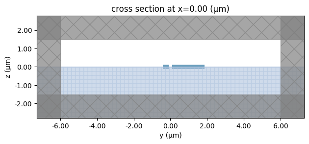
examplesim.plot(x=0)
<Axes: title={'center': 'cross section at x=0.00 (μm)'}, xlabel='y (μm)', ylabel='z (μm)'>
examplesm = makesim(
    sm_width=0.3125,
    mm_width=1.762,
    gap=0.2,
    smon=True,
    mmon=False,
)
examplemm = makesim(
    sm_width=0.3125,
    mm_width=1.762,
    gap=0.2,
    smon=False,
    mmon=True,
)
examplesu = makesim(
    sm_width=0.3125,
    mm_width=1.762,
    gap=0.2,
    smon=True,
    mmon=True,
)
examplebatch = {
    "sm": examplesm,
    "mm": examplemm,
    "su": examplesu,
}
# Uncomment these lines to run an example simulation and show mode plots
exampleresults = web.run(examplebatch)
exampleprocessed = simprocessor(exampleresults, showplots=True)
Output()
13:38:29 KST Started working on Batch containing 3 tasks.
13:38:34 KST Maximum FlexCredit cost: 0.032 for the whole batch.
             Use 'Batch.real_cost()' to get the billed FlexCredit cost after
             completion.
Output()
13:39:13 KST Batch complete.
Sweep Parameters
# Replace these values with your own values of interest
smwids = 0.3125
mmwids = [
    0.3125,
    0.672,
    1.036,
    1.399,
    1.762,
    2.125,
    2.488,
    2.851,
    3.215,
    3.578,
    3.941,
    4.305,
    4.667,
    5.031,
    5.394,
]
gaps = np.arange(50, 300, 50) * 1e-3
Running the Sweep
dat = sweeprunner(
    smwids=smwids,
    mmwids=mmwids,
    gaps=gaps,
)
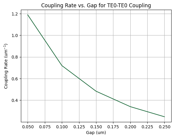
plt.figure()
plt.plot(
    gaps,
    dat["mode0"]["omegas"][:, 0],
)
plt.xlabel("Gap (um)")
plt.ylabel("Coupling Rate (um$^{-1}$)")
plt.title("Coupling Rate vs. Gap for TE0-TE0 Coupling")
plt.grid(True)
plt.show()
Plot Results for General Mode Coupling
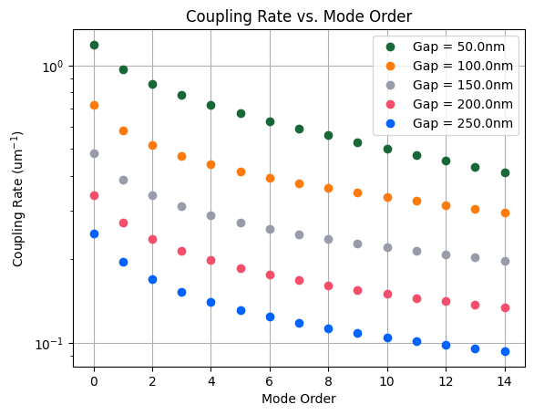
plt.figure()
for j in range(len(gaps)):
    omegapermode = []
    for i in range(len(mmwids)):
        omegapermode.append(np.max(dat["mode" + str(i)]["omegas"][j, :]))

    plt.plot(
        np.arange(0, len(mmwids)),
        omegapermode,
        ls="",
        marker="o",
        label="Gap = " + str(gaps[j] * 1e3) + "nm",
    )
plt.yscale("log")
plt.title("Coupling Rate vs. Mode Order")
plt.xlabel("Mode Order")
plt.ylabel("Coupling Rate (um$^{-1}$)")
plt.grid(True)
plt.legend()
plt.show()


 TERMS & CONDITIONS


 How the process works:
 Try this real URL to see an example: