





Alessandro Mauro and Alfonso Palmieri, Harvard John A. Paulson School of Engineering and Applied Sciences
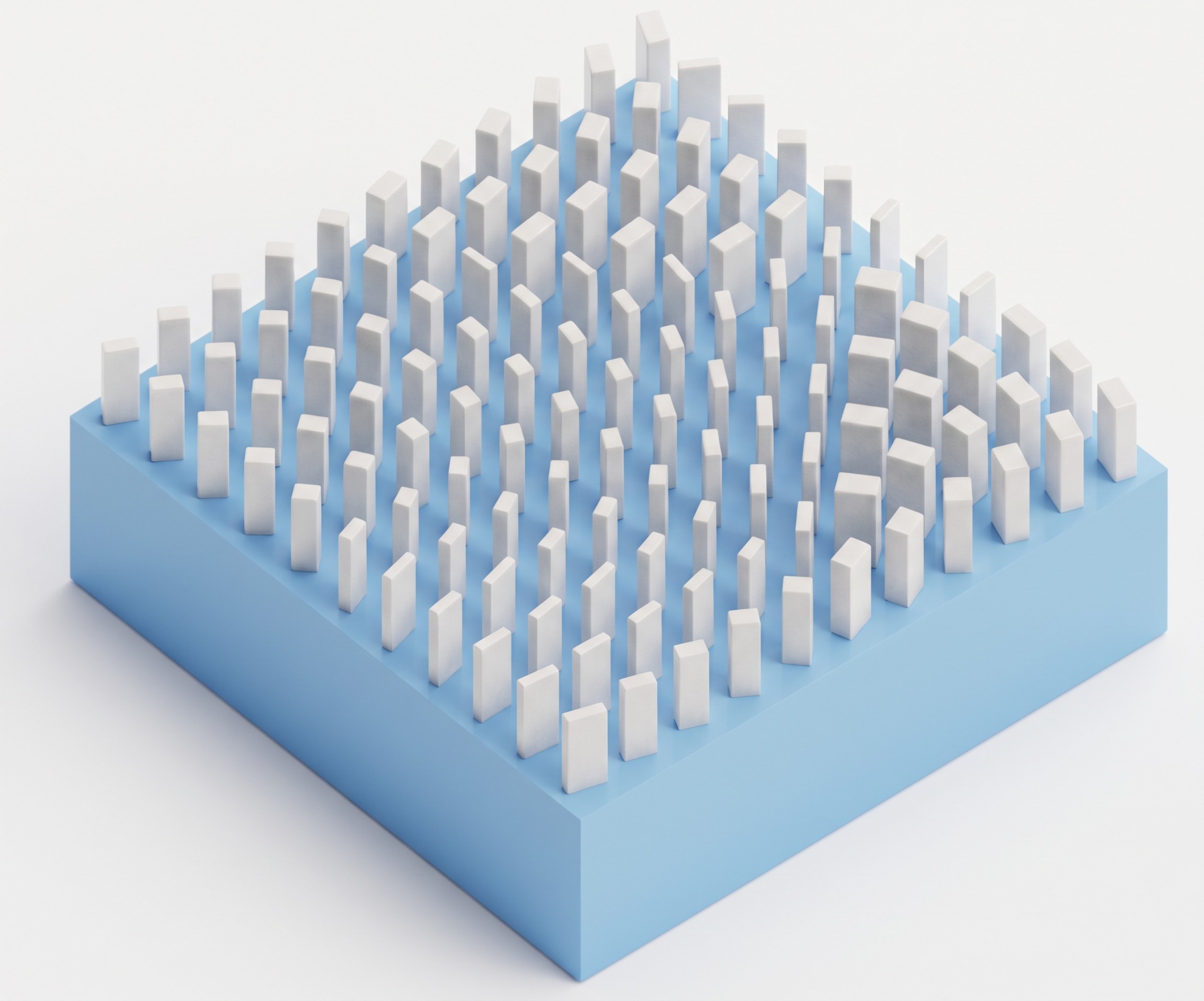
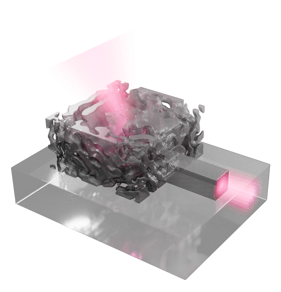
A full measurement of the polarization of light, its four Stokes parameters, normally requires several sequential measurements or a combination of waveplates, polarizers and beam splitters. Rubin et al. showed that a single metasurface can do it in one shot [1]: a periodic array of birefringent nanopillars forms a diffraction grating whose diffraction orders each act as a polarization analyzer for a different state. If the four analyzed states form a tetrahedron on the Poincaré sphere, the four order intensities determine the full Stokes vector, and a camera placed behind the grating becomes a compact full-Stokes polarization camera.
The design rests on matrix Fourier optics: the Jones matrix of the grating is expanded in a Fourier series, and each Fourier coefficient is the Jones matrix of one diffraction order. Choosing the pillar rotations and phase delays so that these coefficients are polarization analyzers turns a polarimetry problem into a constrained optimization problem.
In this notebook we reproduce the full design flow:
- Design scheme. We optimize an $11 \times 11$ supercell of ideal waveplates within the thin-element (Fourier optics) approximation, following the supplement of [1].
- Nanopillar library. We compute with Tidy3D the transmission of rectangular TiO$_2$ pillars on glass at $\lambda_0 = 532$ nm.
- Mapping. Each ideal waveplate of the design is replaced by the library pillar that best reproduces it.
-
Full-wave simulation. We simulate the complete supercell in Tidy3D and extract the Jones matrix of every diffraction order with a
DiffractionMonitor. - Analysis. We verify that the four orders are polarization analyzers for the target states and use them to reconstruct the polarization of the incident light.
The implementation of the design scheme was inspired by the open-source code by N. A. Rubin, Polarization-Grating-Design [2], which accompanies [1]. Here it is re-implemented in Python with explicit conventions, and extended with the pillar library and the full-wave verification in Tidy3D.
The helper functions for plotting, library mapping and post-processing are collected in the Appendix at the end of the notebook and in the companion module misc/mfo_helpers.py, so that the main text follows the physics.
import numpy as np
import matplotlib.pyplot as plt
from scipy.optimize import minimize

import tidy3d as td
import tidy3d.web as web

from misc import mfo_helpers as mh  # plotting, library mapping and post-processing (see the Appendix)
1. Design scheme
1.1 Conventions
Throughout the notebook we use the time dependence $e^{-i\omega t}$ (the same as Tidy3D), propagation along $+z$, and Jones vectors $\mathbf{E} = (E_x, E_y)^T$. The Stokes parameters are
$$ S_0 = |E_x|^2 + |E_y|^2, \quad S_1 = |E_x|^2 - |E_y|^2, \quad S_2 = 2\,\mathrm{Re}(E_x E_y^*), \quad S_3 = 2\,\mathrm{Im}(E_x E_y^*), $$
so that right circular polarization $(1, -i)/\sqrt{2}$ sits at the north pole of the Poincaré sphere ($S_3 = +1$). A unit Stokes vector $\mathbf{s} = (S_1, S_2, S_3)$ corresponds to the Jones vector
$$ |q\rangle = \left(\cos\frac{\chi}{2},\ \sin\frac{\chi}{2}\, e^{-i\psi}\right)^T, \qquad \cos\chi = S_1, \quad \psi = \mathrm{atan2}(S_3, S_2), $$
up to a global phase, and the orthogonal state $|q_\perp\rangle$ is the antipodal point of the sphere.
def stokes_of(E):
    '''Stokes vector (S0, S1, S2, S3) of Jones vectors E (last axis = (Ex, Ey)).'''
    Ex, Ey = E[..., 0], E[..., 1]
    return np.stack([abs(Ex) ** 2 + abs(Ey) ** 2,
                     abs(Ex) ** 2 - abs(Ey) ** 2,
                     2 * (Ex * Ey.conj()).real,
                     2 * (Ex * Ey.conj()).imag], axis=-1)


def jones_from_stokes(s):
    '''Unit Jones vectors with Stokes vectors s (last axis = (S1, S2, S3)); Ex real and >= 0.'''
    s = np.asarray(s, dtype=float)
    s = s / np.linalg.norm(s, axis=-1, keepdims=True)
    chi = np.arccos(np.clip(s[..., 0], -1, 1))
    psi = np.arctan2(s[..., 2], s[..., 1])
    return np.stack([np.cos(chi / 2), np.sin(chi / 2) * np.exp(-1j * psi)], axis=-1)


def perp(q):
    '''Jones vectors orthogonal to q (antipodal points on the Poincaré sphere).'''
    return np.stack([-q[..., 1].conj(), q[..., 0].conj()], axis=-1)


rcp = np.array([1, -1j]) / np.sqrt(2)
print("Stokes vector of RCP:", stokes_of(rcp).round(3) + 0.0)
Stokes vector of RCP: [1. 0. 0. 1.]
1.2 Target analyzers
Four intensity measurements are the minimum needed to determine the four Stokes parameters. The best-conditioned choice is a set of four analyzer states at the vertices of a regular tetrahedron inscribed in the Poincaré sphere [1]. We place one vertex at the north pole (RCP) and the other three at $S_3 = -1/3$, and assign them to the four first orders $(\pm1, 0)$ and $(0, \pm1)$.
ORDERS = [(1, 0), (-1, 0), (0, 1), (0, -1)]


def tetrahedron_stokes():
    '''Unit Stokes vectors of the tetrahedron, one row per order in ORDERS.'''
    phi = np.radians([120, 0, 240])
    r = np.sqrt(8) / 3
    lower = np.column_stack([r * np.cos(phi), r * np.sin(phi), np.full(3, -1 / 3)])
    return np.vstack([lower, [0.0, 0.0, 1.0]])


S = tetrahedron_stokes()  # target Stokes vectors, shape (4, 3)
Q = jones_from_stokes(S)  # target Jones vectors, shape (4, 2)

for o, s in zip(ORDERS, S):
    print(f"order {str(o):>8}:  s = ({s[0]:+.3f}, {s[1]:+.3f}, {s[2]:+.3f})")
order   (1, 0):  s = (-0.471, +0.816, -0.333)
order  (-1, 0):  s = (+0.943, +0.000, -0.333)
order   (0, 1):  s = (-0.471, -0.816, -0.333)
order  (0, -1):  s = (+0.000, +0.000, +1.000)
1.3 Matrix Fourier optics
Consider a metasurface whose local Jones matrix $J(x, y)$ is periodic with periods $d_x$ and $d_y$. Within the thin-element approximation, the field transmitted into the diffraction order $(m, n)$ is $\mathbf{E}_{mn} = J_{mn}\,\mathbf{E}_{\rm in}$, where $J_{mn}$ is a Fourier coefficient of the Jones matrix:
$$ J_{mn} = \frac{1}{d_x d_y} \iint_{\rm cell} J(x, y)\, e^{-i 2\pi \left(m x / d_x + n y / d_y\right)}\, dx\, dy . $$
The minus sign in the exponent is what sends order $+m$ toward $+k_x$ with our $e^{-i\omega t}$ convention.
We want order $k$ to behave as a polarization analyzer for the state $|q_k\rangle$: the transmitted power must be proportional to $|\langle q_k | \mathbf{E}_{\rm in}\rangle|^2$, and it must vanish for the orthogonal state. The metasurface is built from linearly birefringent pillars, whose Jones matrices are symmetric ($J = J^T$). The Fourier coefficients are therefore symmetric too, and the analyzer must take the form
$$ J_{k} = a_k\, |q_k^*\rangle\langle q_k| , $$
so the light leaving order $k$ is always in the state $|q_k^*\rangle$ (the mirror image of $|q_k\rangle$ across the equator), whatever the input.
For a lossless metasurface $J(x, y)$ is unitary, and Parseval's theorem gives $\sum_{mn} J_{mn}^\dagger J_{mn} = \mathbb{1}$: the power is conserved over all orders. For four tetrahedron analyzers of equal strength, $\sum_k J_k^\dagger J_k = 2|a|^2\,\mathbb{1}$. The best possible design therefore has $|a|^2 = 1/2$, i.e. $\sum_k I_q^{(k)} = 2$, with all the light in the four orders.
1.4 Pixelated grating
The supercell is divided into $A \times B$ pixels of pitch $d$, each containing one pillar. Pixel $(a, b)$ is an ideal waveplate with phase delays $\phi_x$ and $\phi_y$ along its own axes, rotated by $\theta$:
$$ J_{ab} = R(\theta_{ab}) \begin{pmatrix} e^{i\phi_{x,ab}} & 0 \\ 0 & e^{i\phi_{y,ab}} \end{pmatrix} R(\theta_{ab})^T . $$
Since $J(x, y)$ is piecewise constant, the Fourier integral becomes a discrete Fourier transform times a sinc envelope from the pixel shape (Eq. S37 of [1]):
$$ J_{mn} = \frac{1}{AB}\,\mathrm{sinc}\!\left(\frac{m}{A}\right)\mathrm{sinc}\!\left(\frac{n}{B}\right) \sum_{a=1}^{A}\sum_{b=1}^{B} J_{ab}\; e^{-i 2\pi \left[m (a - 1/2)/A + n (b - 1/2)/B\right]} . $$
In code, the design is a flat vector of $3AB$ parameters $(\phi_x, \phi_y, \theta)$, and all maps are arrays of shape $(B, A)$ indexed as [b, a].
A = B = 11  # pixels per supercell side


def pack(phix, phiy, theta):
    '''Three (B, A) maps -> one flat parameter vector.'''
    return np.concatenate([phix.ravel(), phiy.ravel(), theta.ravel()])


def unpack(x, A, B):
    '''Flat parameter vector -> (phix, phiy, theta), each of shape (B, A).'''
    phix, phiy, theta = np.asarray(x).reshape(3, B, A)
    return phix, phiy, theta


def pillar_matrices(phix, phiy, theta, tx=1.0, ty=1.0):
    '''Jones matrix of every pixel, shape (B, A, 2, 2): R(theta) diag(tx e^{i phix}, ty e^{i phiy}) R(theta)^T.
    tx = ty = 1 for ideal waveplates, library amplitudes for real pillars.'''
    ex, ey = tx * np.exp(1j * phix), ty * np.exp(1j * phiy)
    c, s = np.cos(theta), np.sin(theta)
    J = np.empty(np.shape(theta) + (2, 2), dtype=complex)
    J[..., 0, 0] = c**2 * ex + s**2 * ey
    J[..., 1, 1] = s**2 * ex + c**2 * ey
    J[..., 0, 1] = J[..., 1, 0] = c * s * (ex - ey)
    return J


def order_weights(orders, A, B):
    '''Weight of every pixel in every order (Eq. S37 without the Jones matrices), shape (K, B, A).'''
    a = np.arange(1, A + 1) - 0.5
    b = np.arange(1, B + 1) - 0.5
    W = np.empty((len(orders), B, A), dtype=complex)
    for k, (m, n) in enumerate(orders):
        envelope = np.sinc(m / A) * np.sinc(n / B) / (A * B)
        W[k] = envelope * np.exp(-2j * np.pi * (n * b[:, None] / B + m * a[None, :] / A))
    return W


def order_jones(J, W):
    '''Jones matrix of every order, shape (K, 2, 2).'''
    return np.einsum("kba,baij->kij", W, J)


W = order_weights(ORDERS, A, B)
1.5 Figures of merit
For each order we evaluate the power transmitted when its own target state is incident, $I_q$, and when the orthogonal state is incident, $I_{q\perp}$ (Eqs. S38 and S39):
$$ I_q^{(k)} = \langle q_k | J_k^\dagger J_k | q_k\rangle, \qquad I_{q\perp}^{(k)} = \langle q_{k\perp} | J_k^\dagger J_k | q_{k\perp}\rangle, \qquad \eta_k = \frac{I_q^{(k)} - I_{q\perp}^{(k)}}{I_q^{(k)} + I_{q\perp}^{(k)}} . $$
A perfect analyzer has contrast $\eta_k = 1$. The optimization problem (Eqs. S41 to S43) is
$$ \max_{\phi_x, \phi_y, \theta}\ \sum_k I_q^{(k)} \quad \text{subject to} \quad \eta_k = 1 \ \ \forall k, \qquad \mathrm{var}\big(I_q^{(k)}\big) = 0 . $$
The second constraint makes the four analyzers equally strong. We use the variance rather than the standard deviation because it is smooth at zero, which the gradient-based optimizer needs.
def I_q(Jk, Q):
    '''Power in each order when its target state is incident.'''
    return np.sum(np.abs(np.einsum("kij,kj->ki", Jk, Q)) ** 2, axis=1)


def contrast(Jk, Q):
    '''(I_q - I_qperp) / (I_q + I_qperp) for each order.'''
    iq, ip = I_q(Jk, Q), I_q(Jk, perp(Q))
    return (iq - ip) / (iq + ip)


def orders_from_x(x, W, A, B):
    return order_jones(pillar_matrices(*unpack(x, A, B)), W)


def merit(x, W, Q, A, B):
    '''Sum of the I_q over the four orders, to be maximized.'''
    return I_q(orders_from_x(x, W, A, B), Q).sum()


def constraints(x, W, Q, A, B):
    '''Equality constraints, all zero at a valid design: contrast - 1 for each order, variance of the I_q.'''
    Jk = orders_from_x(x, W, A, B)
    return np.append(contrast(Jk, Q) - 1, np.var(I_q(Jk, Q)))
1.6 Optimization
We maximize the merit with sequential least-squares programming (SLSQP) from scipy, starting from several random designs, and keep the best run that satisfies all the constraints. The problem has $3AB = 363$ variables; the full multi-start takes a few minutes on a laptop.
def evaluate(x, W, Q, A, B):
    Jk = orders_from_x(x, W, A, B)
    iq = I_q(Jk, Q)
    return {"merit": iq.sum(), "I_q": iq, "contrast": contrast(Jk, Q), "var": np.var(iq)}


def optimize(seed, W, Q, A, B, maxiter=1000, ftol=1e-9):
    '''One SLSQP run from a random design; returns the final design and the history of the metrics.'''
    rng = np.random.default_rng(seed)
    phix, phiy = rng.uniform(0, 2 * np.pi, (2, B, A))
    theta = rng.uniform(0, np.pi, (B, A))
    x0 = pack(phix, phiy, theta)

    args = (W, Q, A, B)
    history = [evaluate(x0, *args)]
    res = minimize(lambda x: -merit(x, *args), x0, method="SLSQP",
                   constraints={"type": "eq", "fun": constraints, "args": args},
                   options={"maxiter": maxiter, "ftol": ftol},
                   callback=lambda xk: history.append(evaluate(xk, *args)))
    history = {key: np.array([h[key] for h in history]) for key in history[0]}
    violation = np.max(np.abs(constraints(res.x, *args)))
    return {"seed": seed, "x": res.x, "history": history, "violation": violation}


runs = [optimize(seed, W, Q, A, B) for seed in range(5)]
for r in runs:
    print(f"seed {r['seed']}:  merit = {r['history']['merit'][-1]:.4f}   max constraint violation = {r['violation']:.1e}")

best = max((r for r in runs if r["violation"] < 1e-3), key=lambda r: r["history"]["merit"][-1])
print(f"\nbest design: seed {best['seed']}")
seed 0:  merit = 1.6651   max constraint violation = 1.5e-10
seed 1:  merit = 1.6651   max constraint violation = 8.1e-11
seed 2:  merit = 1.6651   max constraint violation = 6.6e-11
seed 3:  merit = 1.6651   max constraint violation = 8.5e-11
seed 4:  merit = 1.6651   max constraint violation = 1.4e-10

best design: seed 1
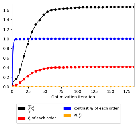
The convergence of the best run reproduces Fig. S10 of [1]: the contrast of all four orders reaches 1 within a few iterations, and the merit then grows for about 100 iterations to $\sum_k I_q \approx 1.665$, close to the value of 1.65 reported in the paper and below the bound of 2 derived above. All five random starts converge to the same merit.
mh.plot_convergence(best["history"])
1.7 The ideal design
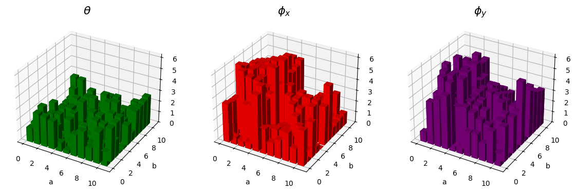
The optimized supercell, pixel by pixel (Fig. S8):
phix_t, phiy_t, theta = unpack(best["x"], A, B)
mh.plot_design(phix_t, phiy_t, theta)

Jk_ideal = order_jones(pillar_matrices(phix_t, phiy_t, theta), W)
eff_ideal = 2 * I_q(Jk_ideal, Q).mean()  # fraction of the power in the four orders, for any input

print("order        I_q     contrast")
for k, o in enumerate(ORDERS):
    print(f"{str(o):>8}   {I_q(Jk_ideal, Q)[k]:.4f}   {contrast(Jk_ideal, Q)[k]:.4f}")
print(f"\nfraction of the incident power in the four orders: {eff_ideal:.4f} (the same for every input polarization)")
order        I_q     contrast
  (1, 0)   0.4163   1.0000
 (-1, 0)   0.4163   1.0000
  (0, 1)   0.4163   1.0000
 (0, -1)   0.4163   1.0000

fraction of the incident power in the four orders: 0.8325 (the same for every input polarization)
With perfect analyzers of equal strength, $\sum_k J_k^\dagger J_k \propto \mathbb{1}$, so the power collected by the four orders does not depend on the input polarization. The rest of the light goes to the zero order and to higher orders.
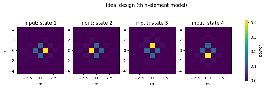
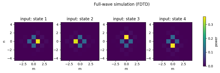
To see the analyzers at work, we send each of the four target states onto the grating and plot the power in all orders with $|m|, |n| \le 4$ (Fig. S11). For input state $k$, order $k$ is bright, and the other three orders receive the same smaller power, because the tetrahedron states are equidistant on the sphere.
M = 4
ms = ns = np.arange(-M, M + 1)
grid_orders = [(m, n) for n in ns for m in ms]
Jgrid_ideal = order_jones(pillar_matrices(phix_t, phiy_t, theta), order_weights(grid_orders, A, B))
Jgrid_ideal = Jgrid_ideal.reshape(len(ns), len(ms), 2, 2)

P_ideal = [np.sum(np.abs(np.einsum("nmij,j->nmi", Jgrid_ideal, q)) ** 2, axis=-1) for q in Q]
mh.plot_order_maps(ms, ns, P_ideal, "Ideal design (thin-element model)")
2. Nanopillar library
The design assumes ideal waveplates. To build it, we need real pillars whose transmission reproduces the required $(\phi_x, \phi_y)$ pairs. We use rectangular TiO$_2$ pillars, $600$ nm tall, on a glass substrate ($n = 1.4$), on a square lattice with $420$ nm pitch, at $\lambda_0 = 532$ nm. The refractive index of TiO$_2$ ($n = 2.4506$) comes from ellipsometry of deposited films; absorption is neglected.
Each library entry is a periodic unit cell with one pillar of sides $D_x \times D_y$, illuminated by an $x$-polarized plane wave from the substrate. Since the pitch is smaller than the wavelength in air, only the zero order propagates in transmission, and its complex amplitude is the average of $E_x$ over a plane above the pillar. We normalize it to the same quantity computed for the bare substrate, so that the library contains only the effect of the pillar. The mirror symmetry of the unit cell and of the source lets us simulate only a quarter of it.
We use a uniform grid of $10$ nm, the same that we will use for the full supercell.
nm = 1e-3  # Tidy3D lengths are in µm

lambda0 = 532 * nm
freq0 = td.C_0 / lambda0
fwidth = freq0 / 10
run_time = 200 / fwidth

period = 420 * nm
h_pillar = 600 * nm
n_sub = 1.4
n_tio2 = 2.4506  # ellipsometry, 532 nm
dl = 10 * nm

glass = td.Medium(permittivity=n_sub**2, name="glass")
tio2 = td.Medium(permittivity=n_tio2**2, name="TiO2")

# vertical layout: z = 0 is the glass/air interface
z_src = -lambda0 / 2  # plane-wave source, in the glass
z_rfl = z_src - lambda0 / 2  # reflection monitors
z_top = h_pillar  # top of the pillars
z_pad = 1.5 * lambda0  # space before the PML
substrate = td.Structure(
    geometry=td.Box(center=(0, 0, -5 * lambda0), size=(td.inf, td.inf, 10 * lambda0)),
    medium=glass,
    name="substrate",
)
z_lib_mon = z_top + lambda0 / 2
z_lib_min, z_lib_max = z_rfl - z_pad, z_lib_mon + z_pad

lib_source = td.PlaneWave(
    source_time=td.GaussianPulse(freq0=freq0, fwidth=fwidth),
    size=(td.inf, td.inf, 0),
    center=(0, 0, z_src),
    direction="+",
    pol_angle=0,
)

lib_monitor = td.FieldMonitor(
    center=(0, 0, z_lib_mon),
    size=(td.inf, td.inf, 0),
    freqs=[freq0],
    fields=["Ex"],
    name="field",
)


def make_library_sim(Dx=None, Dy=None):
    '''Unit cell with one Dx x Dy pillar; no pillar (reference) if Dx is None.'''
    structures = [substrate]
    if Dx is not None:
        pillar = td.Box(center=(0, 0, h_pillar / 2), size=(Dx, Dy, h_pillar))
        structures.append(td.Structure(geometry=pillar, medium=tio2))
    return td.Simulation(
        size=(period, period, z_lib_max - z_lib_min),
        center=(0, 0, (z_lib_max + z_lib_min) / 2),
        structures=structures,
        sources=[lib_source],
        monitors=[lib_monitor],
        grid_spec=td.GridSpec.uniform(dl=dl),
        run_time=run_time,
        boundary_spec=td.BoundarySpec.pml(z=True),  # periodic in x and y
        symmetry=(-1, 1, 0),
    )


sim_example = make_library_sim(150 * nm, 200 * nm)
fig, axs = plt.subplots(1, 2, figsize=(9, 5), gridspec_kw={"width_ratios": [1, 1.6]})
sim_example.plot(y=0, ax=axs[0])
axs[0].set_xticks([-0.2, 0.2])
sim_example.plot(z=h_pillar / 2, ax=axs[1])
plt.tight_layout()
plt.show()
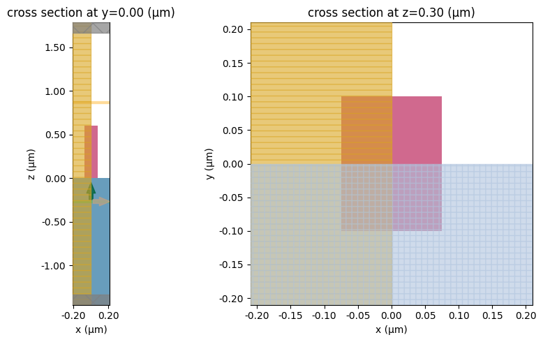
The sweep covers $D_x, D_y$ from $50$ to $250$ nm in $5$ nm steps: $41 \times 41 = 1681$ small simulations, about $42$ FlexCredits in total. The code below runs it when run_library = True; by default, it loads the result of that same sweep from misc/pillar_library.npz.
sides = np.round(np.arange(50, 250.1, 5) * nm, 6)
library_file = "misc/pillar_library.npz"
run_library = False


def zero_order(sim_data):
    '''Complex zero-order transmission: average of Ex over one period (the last grid point repeats the first).'''
    Ex = sim_data["field"].Ex.isel(f=0, z=0)
    return complex(Ex.isel(x=slice(0, -1), y=slice(0, -1)).mean())


if run_library:
    key = lambda Dx, Dy: f"Dx{round(Dx / nm):03d}_Dy{round(Dy / nm):03d}"
    sims = {key(Dx, Dy): make_library_sim(Dx, Dy) for Dx in sides for Dy in sides}
    sims["reference"] = make_library_sim()
    batch_lib = web.Batch(simulations=sims, folder_name="MFO_library")
    print(f"estimated cost: {batch_lib.estimate_cost():.1f} FlexCredits")
    lib_data = batch_lib.run(path_dir="data/library")

    t_ref_lib = zero_order(lib_data["reference"])
    t = np.array([[zero_order(lib_data[key(Dx, Dy)]) / t_ref_lib for Dy in sides] for Dx in sides])
    np.savez(library_file, sides=sides, amp=np.abs(t), phase=np.angle(t))

lib_raw = np.load(library_file)
lib = mh.load_library(library_file)
mh.plot_library(lib_raw["sides"], lib_raw["amp"], lib_raw["phase"])
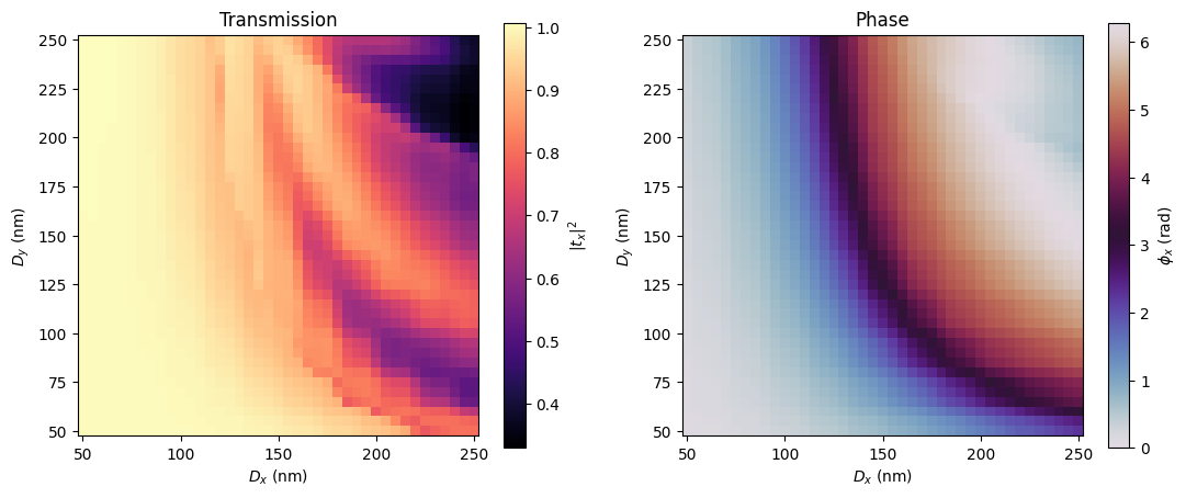
Elongated pillars behave as waveplates: the phase along the long side is larger than along the short side, and the difference can reach $\pi$. The transmission stays above $\sim 0.5$ over most of the map, with dips at resonances of the larger pillars.
3. From the ideal design to real pillars
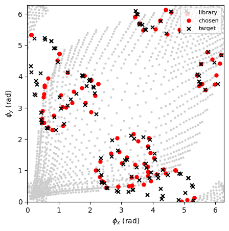
Each pixel is assigned to the library pillar that best reproduces its complex transmissions $e^{i\phi_x}$ and $e^{i\phi_y}$ (Eq. S44), up to a phase offset $c$ that is common to the whole supercell and chosen to minimize the total error (see map_to_library in the Appendix). The pillar is then rotated by the design angle $\theta$. The resulting supercell is shown in Section 4.
idx, c_best, err = mh.map_to_library(phix_t, phiy_t, lib)
Dx, Dy = lib["Dx"][idx], lib["Dy"][idx]  # chosen pillars, shape (B, A)

print(f"common offset c = {np.degrees(c_best):.1f} deg")
print(f"mapping error: mean {err.mean():.4f}, worst pixel {err.max():.4f}")
print(f"pillar sides from {1e3 * min(Dx.min(), Dy.min()):.0f} to {1e3 * max(Dx.max(), Dy.max()):.0f} nm")

mh.plot_phase_plane(lib, idx, phix_t, phiy_t, c_best)
common offset c = 184.0 deg
mapping error: mean 0.0521, worst pixel 0.2410
pillar sides from 55 to 250 nm
Before running the full-wave simulation, we can predict the performance of the real supercell with the same Fourier model, now using the measured amplitudes and phases of the chosen pillars. This library model includes the loss and phase errors of the pillars, but still neglects the coupling between neighbouring pillars that are different from each other.
J_lib = pillar_matrices(lib["phix"][idx], lib["phiy"][idx], theta, tx=lib["tx"][idx], ty=lib["ty"][idx])
Jk_lib = order_jones(J_lib, W)

print("order      I_q ideal   I_q library    contrast ideal   contrast library")
for k, o in enumerate(ORDERS):
    print(f"{str(o):>8}     {I_q(Jk_ideal, Q)[k]:.3f}       {I_q(Jk_lib, Q)[k]:.3f}"
          f"          {contrast(Jk_ideal, Q)[k]:.4f}           {contrast(Jk_lib, Q)[k]:.4f}")
order      I_q ideal   I_q library    contrast ideal   contrast library
  (1, 0)     0.416       0.347          1.0000           0.9966
 (-1, 0)     0.416       0.340          1.0000           0.9967
  (0, 1)     0.416       0.359          1.0000           0.9988
 (0, -1)     0.416       0.346          1.0000           0.9990
4. Full-wave simulation of the supercell
We now simulate the complete $11 \times 11$ supercell, $4.62 \times 4.62$ µm$^2$ with 121 rotated pillars, with periodic boundary conditions in $x$ and $y$. The first diffraction orders leave the grating at $\arcsin(\lambda_0 / 4.62\,\mu\text{m}) \approx 6.6°$.
4.1 Geometry
Each pillar is a PolySlab: the four corners of a $D_x \times D_y$ rectangle, rotated by $\theta$ and moved to the centre of its pixel.
Lx, Ly = A * period, B * period

aa, bb = np.meshgrid(np.arange(A), np.arange(B))  # same [b, a] order as the design maps
xc = (-Lx / 2 + (aa + 0.5) * period).ravel()
yc = (-Ly / 2 + (bb + 0.5) * period).ravel()
dx, dy, th = Dx.ravel() / 2, Dy.ravel() / 2, theta.ravel()

corners = np.stack([np.column_stack([+dx, +dy]), np.column_stack([-dx, +dy]),
                    np.column_stack([-dx, -dy]), np.column_stack([+dx, -dy])], axis=1)  # (N, 4, 2)
rotation = np.array([[np.cos(th), -np.sin(th)], [np.sin(th), np.cos(th)]])  # (2, 2, N)
vertices = np.einsum("nij,kjn->nik", corners, rotation) + np.column_stack([xc, yc])[:, None, :]

pillars = td.Structure(
    geometry=td.GeometryGroup(
        geometries=[td.PolySlab(vertices=v, slab_bounds=(0, h_pillar), axis=2) for v in vertices]
    ),
    medium=tio2,
    name="pillars",
)

side_x = vertices[:, 0] - vertices[:, 1]  # the Dx side of every pillar
assert np.allclose(np.linalg.norm(side_x, axis=1), Dx.ravel())
assert np.allclose(np.mod(np.arctan2(side_x[:, 1], side_x[:, 0]) - th + np.pi / 2, np.pi) - np.pi / 2, 0)
4.2 Sources and monitors
A normally incident plane wave is launched from the substrate. Two simulations, with $x$ and $y$ polarization, give the two columns of the Jones matrix of every order.
The monitors are:
- a
DiffractionMonitorabove the pillars, which decomposes the transmitted field into diffraction orders, with the complex amplitude of both polarizations of each order; - a
DiffractionMonitorin the substrate for the reflected orders; - two
FluxMonitors to check the energy balance; - a
FieldMonitorin the $xz$ plane to visualize the near field.
The transmission monitor is placed 1 µm above the pillars, far enough for the evanescent orders to have decayed.
z_diff = z_top + 1.0
z_min, z_max = z_rfl - z_pad, z_diff + z_pad

source_x = td.PlaneWave(
    source_time=td.GaussianPulse(freq0=freq0, fwidth=fwidth),
    size=(td.inf, td.inf, 0),
    center=(0, 0, z_src),
    direction="+",
    pol_angle=0,
)
source_y = source_x.updated_copy(pol_angle=np.pi / 2)

diff_T = td.DiffractionMonitor(
    center=(0, 0, z_diff), size=(td.inf, td.inf, 0), freqs=[freq0], normal_dir="+", name="diff_T"
)
diff_R = td.DiffractionMonitor(
    center=(0, 0, z_rfl), size=(td.inf, td.inf, 0), freqs=[freq0], normal_dir="-", name="diff_R"
)
flux_T = td.FluxMonitor(center=(0, 0, z_diff), size=(td.inf, td.inf, 0), freqs=[freq0], name="flux_T")
flux_R = td.FluxMonitor(center=(0, 0, z_rfl), size=(td.inf, td.inf, 0), freqs=[freq0], name="flux_R")
field_xz = td.FieldMonitor(
    center=(0, 0, 0), size=(td.inf, 0, td.inf), freqs=[freq0], fields=["Ex"], name="field_xz"
)
4.3 Simulations
We also run a reference simulation of the bare substrate. Its zero-order amplitude $t_{\rm ref}$ is the transmission of the plain glass/air interface, and dividing by it normalizes the FDTD Jones matrices in the same way as the library.
sim_x = td.Simulation(
    size=(Lx, Ly, z_max - z_min),
    center=(0, 0, (z_max + z_min) / 2),
    structures=[substrate, pillars],
    sources=[source_x],
    monitors=[diff_T, diff_R, flux_T, flux_R, field_xz],
    grid_spec=td.GridSpec.uniform(dl=dl),
    run_time=run_time,
    boundary_spec=td.BoundarySpec.pml(z=True),  # periodic in x and y
)
sim_y = sim_x.updated_copy(sources=[source_y])
sim_ref = sim_x.updated_copy(size=(period, period, z_max - z_min), structures=[substrate], monitors=[diff_T])

print(f"grid: {sim_x.num_cells / 1e6:.1f} million cells")

fig, axs = plt.subplots(1, 2, figsize=(12, 5))
sim_x.plot(z=h_pillar / 2, ax=axs[0])
sim_x.plot(y=0, ax=axs[1])
plt.tight_layout()
plt.show()
grid: 84.7 million cells
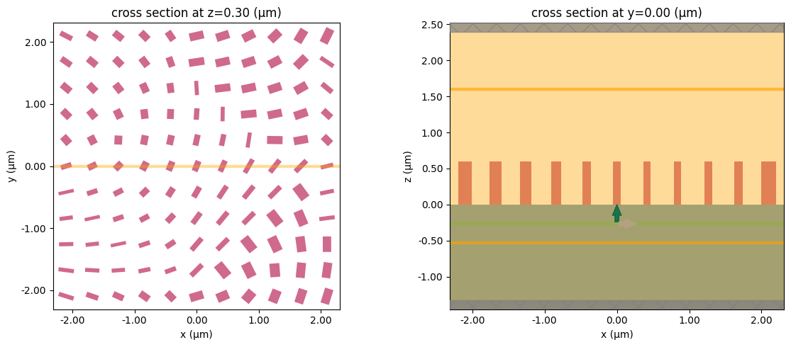
The three simulations are submitted together as a Batch.
td.config.vgpu.priority = 9
td.config.run.pay_type = "FLEX_CREDIT"

batch = web.Batch(simulations={"x": sim_x, "y": sim_y, "ref": sim_ref}, folder_name="MFO_supercell")
print(f"estimated cost: {batch.estimate_cost():.2f} FlexCredits")
00:03:15 EDT Maximum FlexCredit cost: 9.144 for the whole batch.
estimated cost: 9.14 FlexCredits
batch_data = batch.run(path_dir="data/supercell")
Output()
Started working on Batch containing 3 tasks.
00:03:20 EDT Maximum FlexCredit cost: 9.144 for the whole batch.
             Use 'Batch.real_cost()' to get the billed FlexCredit cost after
             completion.
Output()
00:03:22 EDT Batch complete.
data = {"x": batch_data["x"], "y": batch_data["y"]}

fig, ax = plt.subplots(figsize=(10, 5))
data["x"].plot_field("field_xz", "Ex", val="real", ax=ax)
plt.show()
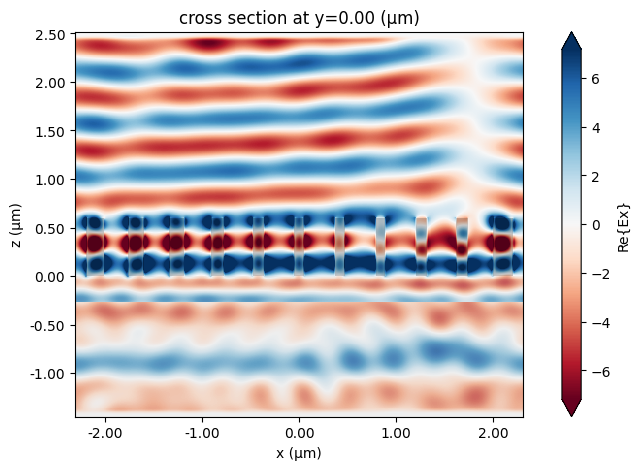
The diffraction angle of the four orders matches the grating equation, and transmitted plus reflected power adds up to one: the simulation is converged and the mesh resolves the structure.
mon = data["x"]["diff_T"]
angle = np.degrees(mon.angles[0].isel(f=0))

print("order     angle (deg)   power, x input   power, y input")
for m, n in ORDERS:
    p = [float(data[pol]["diff_T"].power.isel(f=0).sel(orders_x=m, orders_y=n)) for pol in ("x", "y")]
    print(f"{str((m, n)):>8}      {float(angle.sel(orders_x=m, orders_y=n)):.2f}          {p[0]:.4f}           {p[1]:.4f}")
print(f"grating equation: {np.degrees(np.arcsin(lambda0 / Lx)):.2f} deg\n")

for pol in ("x", "y"):
    T = float(data[pol]["flux_T"].flux.isel(f=0))
    R = -float(data[pol]["flux_R"].flux.isel(f=0))
    print(f"{pol} input:  transmitted {T:.4f}   reflected {R:.4f}   total {T + R:.4f}")
order     angle (deg)   power, x input   power, y input
  (1, 0)      6.61          0.0913           0.2456
 (-1, 0)      6.61          0.3187           0.0089
  (0, 1)      6.61          0.0937           0.2533
 (0, -1)      6.61          0.1771           0.1648
grating equation: 6.61 deg

x input:  transmitted 0.8033   reflected 0.1963   total 0.9996
y input:  transmitted 0.8051   reflected 0.1946   total 0.9997
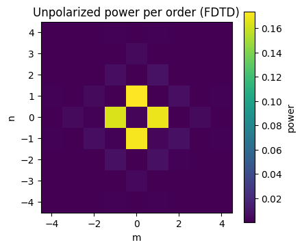
The (unpolarized) power over all transmitted orders, averaged over the $x$ and $y$ runs, shows that most of the light goes into the four first orders.
P_unpol = sum(data[pol]["diff_T"].power.isel(f=0).sel(orders_x=slice(-M, M), orders_y=slice(-M, M))
              for pol in ("x", "y")) / 2

fig, ax = plt.subplots(figsize=(4.5, 4))
pc = ax.pcolormesh(P_unpol.orders_x, P_unpol.orders_y, P_unpol.values.T, shading="auto")
fig.colorbar(pc, ax=ax, label="power")
ax.set(xlabel="m", ylabel="n", aspect="equal", title="Unpolarized power per order (FDTD)")
plt.show()
5.2 Jones matrix of each order
From the two runs we build the Jones matrix of every order (see order_jones_fdtd in the Appendix) and normalize it with the bare-substrate reference. The table compares the three levels of description: the ideal design, the library model, and the full-wave simulation.
mon_ref = batch_data["ref"]["diff_T"]
t_ref = complex(mon_ref.amps.isel(f=0).sel(orders_x=0, orders_y=0, polarization="p"))
Jk_fdtd = np.array([mh.order_jones_fdtd(data, m, n) for m, n in ORDERS]) / t_ref

print(f"bare interface transmission |t_ref|^2 = {abs(t_ref) ** 2:.4f}\n")
print("                    I_q                          contrast")
print("order      ideal  library  FDTD          ideal   library  FDTD")
for k, o in enumerate(ORDERS):
    print(f"{str(o):>8}   {I_q(Jk_ideal, Q)[k]:.3f}   {I_q(Jk_lib, Q)[k]:.3f}   {I_q(Jk_fdtd, Q)[k]:.3f}"
          f"         {contrast(Jk_ideal, Q)[k]:.4f}  {contrast(Jk_lib, Q)[k]:.4f}  {contrast(Jk_fdtd, Q)[k]:.4f}")
bare interface transmission |t_ref|^2 = 0.9725

                    I_q                          contrast
order      ideal  library  FDTD          ideal   library  FDTD
  (1, 0)   0.416   0.347   0.346         1.0000  0.9966  0.9953
 (-1, 0)   0.416   0.340   0.336         1.0000  0.9967  0.9979
  (0, 1)   0.416   0.359   0.357         1.0000  0.9988  0.9989
 (0, -1)   0.416   0.346   0.351         1.0000  0.9990  0.9986
The FDTD results follow the library model closely: the intensities agree within $1$ to $2\%$ and the contrast stays above $0.99$. The drop from the ideal $I_q \approx 0.42$ to $\approx 0.35$ comes almost entirely from the imperfect transmission of the library pillars, not from coupling between neighbouring pillars. This validates the thin-element, library-based design for this supercell.
The diffraction pattern for each target state (Fig. S11) confirms the analyzer behaviour in the full-wave simulation.
Jgrid_fdtd = np.array([[mh.order_jones_fdtd(data, m, n) for m in ms] for n in ns]) / t_ref
P_fdtd = [np.sum(np.abs(np.einsum("nmij,j->nmi", Jgrid_fdtd, q)) ** 2, axis=-1) for q in Q]
mh.plot_order_maps(ms, ns, P_fdtd, "Full-wave simulation (FDTD)")
5.3 Efficiency over the Poincaré sphere
The fraction of the incident power that ends up in the four orders, for every input polarization (Fig. S12). For the ideal design it is constant; with real pillars it varies slightly over the sphere.
th_s, ph_s = np.meshgrid(np.linspace(0, np.pi, 61), np.linspace(0, 2 * np.pi, 121), indexing="ij")
s1, s2, s3 = np.sin(th_s) * np.cos(ph_s), np.sin(th_s) * np.sin(ph_s), np.cos(th_s)
E_sphere = jones_from_stokes(np.stack([s1, s2, s3], axis=-1))


def efficiency(Jk):
    return np.sum(np.abs(np.einsum("kij,...j->k...i", Jk, E_sphere)) ** 2, axis=(0, -1))


eff_lib, eff_fdtd = efficiency(Jk_lib), efficiency(Jk_fdtd)
mh.plot_sphere_map(s1, s2, s3, eff_fdtd, "power in the four orders")

print(f"ideal:    {eff_ideal:.3f}")
print(f"library:  {eff_lib.min():.3f} to {eff_lib.max():.3f}")
print(f"FDTD:     {eff_fdtd.min():.3f} to {eff_fdtd.max():.3f}")
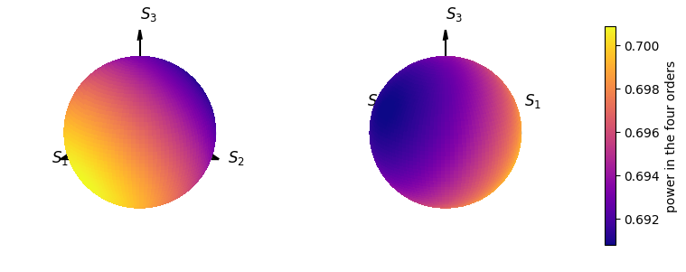
ideal:    0.833
library:  0.690 to 0.704
FDTD:     0.691 to 0.701
5.4 Realized analyzers
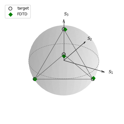
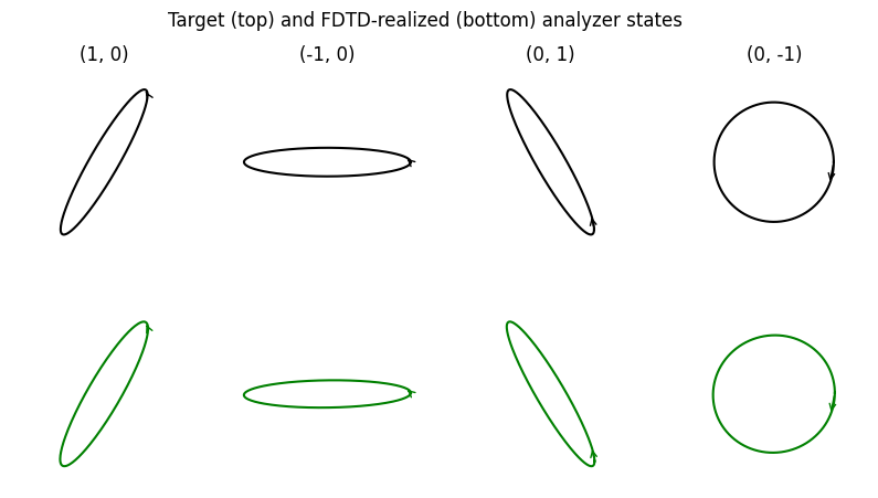
The first row of the Mueller matrix of an order gives the Stokes vector it analyzes (its direction) and its diattenuation (its length divided by $M_{00}$; $1$ for a perfect polarizer). Both are close to the design: the realized analyzers are within a few degrees of the tetrahedron vertices (Fig. 2D).
Mk = np.array([mh.jones_to_mueller(J) for J in Jk_fdtd])
row = Mk[:, 0, 1:]
S_real = row / np.linalg.norm(row, axis=1, keepdims=True)
diattenuation = np.linalg.norm(row, axis=1) / Mk[:, 0, 0]
distance = np.degrees(np.arccos(np.clip(np.sum(S_real * S, axis=1), -1, 1)))

for k, o in enumerate(ORDERS):
    print(f"order {str(o):>8}:  diattenuation {diattenuation[k]:.4f}   distance from target {distance[k]:.2f} deg")

mh.plot_analyzers(S, S_real)
mh.plot_ellipses(Q, jones_from_stokes(S_real), [str(o) for o in ORDERS])
order   (1, 0):  diattenuation 0.9967   distance from target 2.98 deg
order  (-1, 0):  diattenuation 0.9983   distance from target 1.71 deg
order   (0, 1):  diattenuation 0.9990   distance from target 0.82 deg
order  (0, -1):  diattenuation 0.9994   distance from target 2.31 deg
5.5 Output polarization
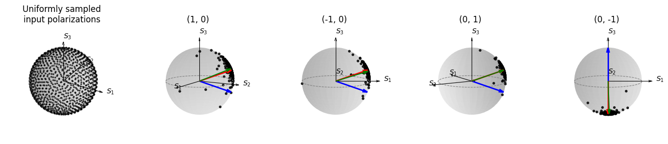
A polarization analyzer $a|q^*\rangle\langle q|$ sends out the same state $|q^*\rangle$ whatever the input. We send 1024 input states, uniformly spread over the Poincaré sphere, through each order (Fig. 2E). The output states (black) collapse around $q^*$ (red), the mirror image of the analyzed state $q$ (blue) across the equator. The green arrow is the power-weighted average output.
s_in = mh.sample_sphere(1024)
E_in = jones_from_stokes(s_in)

outputs = []
for k, o in enumerate(ORDERS):
    S_out = stokes_of(E_in @ Jk_fdtd[k].T)
    avg = S_out[:, 1:].sum(axis=0)
    avg /= np.linalg.norm(avg)
    outputs.append((S_out[:, 1:] / S_out[:, :1], avg))
    q_star = S[k] * [1, 1, -1]
    print(f"order {str(o):>8}:  angle between average output and q* = {np.degrees(np.arccos(np.clip(avg @ q_star, -1, 1))):.2f} deg")

mh.plot_output_states(s_in, outputs, S, [str(o) for o in ORDERS])
order   (1, 0):  angle between average output and q* = 2.82 deg
order  (-1, 0):  angle between average output and q* = 2.67 deg
order   (0, 1):  angle between average output and q* = 3.78 deg
order  (0, -1):  angle between average output and q* = 2.38 deg
5.6 Measuring polarization
Finally, we use the grating as a polarimeter. The power in order $k$ is $I_k = \sum_j M^{(k)}_{0j} S_j$, so the four order powers are related to the incident Stokes vector by the $4 \times 4$ instrument matrix $\mathcal{A}$, whose rows are the first rows of the four Mueller matrices:
$$ \mathbf{I} = \mathcal{A}\,\mathbf{S} \quad\Longrightarrow\quad \mathbf{S} = \mathcal{A}^{-1}\mathbf{I} . $$
We reconstruct the Stokes vectors of the two FDTD inputs, $x$ ($\mathbf{s} = (1, 0, 0)$) and $y$ ($\mathbf{s} = (-1, 0, 0)$), from the order powers recorded by the DiffractionMonitor, first with the instrument matrix of the ideal design and then with the one of the simulated device. In an experiment, the latter corresponds to a calibration of the fabricated grating.
A_ideal = np.array([mh.jones_to_mueller(J)[0] for J in Jk_ideal])
A_fdtd = Mk[:, 0, :]

for pol in ("x", "y"):
    P = np.array([float(data[pol]["diff_T"].power.isel(f=0).sel(orders_x=m, orders_y=n)) for m, n in ORDERS])
    P = P / abs(t_ref) ** 2  # same normalization as the Jones matrices
    for name, A_ins in [("ideal", A_ideal), ("calibrated", A_fdtd)]:
        s = np.linalg.solve(A_ins, P)
        print(f"{pol} input, {name:>10} instrument matrix:  S0 = {s[0]:.3f}   s = {np.round(s[1:] / s[0], 3)}")
x input,      ideal instrument matrix:  S0 = 0.841   s = [ 0.94  -0.009  0.041]
x input, calibrated instrument matrix:  S0 = 1.000   s = [ 1. -0.  0.]
y input,      ideal instrument matrix:  S0 = 0.831   s = [-1.012 -0.028 -0.02 ]
y input, calibrated instrument matrix:  S0 = 1.000   s = [-1.  0. -0.]
With the ideal instrument matrix the polarization state is already recovered within about $5\%$, while the total power is underestimated by about $16\%$ because the real pillars are less efficient than ideal waveplates. With the calibrated matrix the reconstruction is exact, which confirms that the power and amplitude data of the DiffractionMonitor are consistent.
Conclusion
We designed and verified a metasurface polarization grating for full-Stokes polarimetry, following the matrix Fourier optics approach of Rubin et al. [1]. The thin-element optimization reaches $\sum_k I_q \approx 1.66$ with perfect analyzers of equal strength. Mapped onto a library of TiO$_2$ pillars computed with Tidy3D, and simulated in full with 121 rotated pillars, the grating keeps a contrast above $0.99$, analyzes polarization states within a few degrees of the target tetrahedron, and sends about $70\%$ of the incident power into the four analyzer orders for any input polarization. The full-wave results agree with the library model within $1$ to $2\%$, which shows that the library-based design is reliable for this device.
The same workflow applies to other analyzer sets (for example the octahedron of six states), other wavelengths and materials, or larger supercells; only the targets, the library and the grid need to change.
References
[1] N. A. Rubin, G. D'Aversa, P. Chevalier, Z. Shi, W. T. Chen, and F. Capasso, "Matrix Fourier optics enables a compact full-Stokes polarization camera," Science 365, eaax1839 (2019). DOI: 10.1126/science.aax1839
[2] N. A. Rubin, Polarization-Grating-Design, GitHub repository, https://github.com/noahrbn/Polarization-Grating-Design
Appendix: helper functions
These cells contain the full source of misc/mfo_helpers.py, the module imported in the setup cell. Running them rewrites the file, so any change made here takes effect after restarting the kernel.
A.1 Polarization utilities
The Mueller matrix of a Jones matrix, $M_{ij} = \frac{1}{2}\mathrm{Tr}\left(\tau_i J \tau_j J^\dagger\right)$, with the Pauli matrices ordered to match our Stokes convention, and a quasi-uniform sampling of the Poincaré sphere.
%%writefile misc/mfo_helpers.py
"""Helper functions for the matrix Fourier optics polarization grating example.

The notebook imports this module in its setup cell; the same code is listed and
explained in the notebook Appendix, and running the Appendix rewrites this file."""
import numpy as np
import matplotlib.pyplot as plt
from matplotlib.colors import Normalize
import tidy3d as td

# Pauli matrices in the order of our Stokes vector:
# S1 = |Ex|^2 - |Ey|^2,  S2 = 2 Re(Ex Ey*),  S3 = 2 Im(Ex Ey*)
TAU = np.array([[[1, 0], [0, 1]],
                [[1, 0], [0, -1]],
                [[0, 1], [1, 0]],
                [[0, 1j], [-1j, 0]]], dtype=complex)


def jones_to_mueller(J):
    """4 x 4 Mueller matrix of a 2 x 2 Jones matrix."""
    return 0.5 * np.einsum("iab,bc,jcd,da->ij", TAU, J, TAU, J.conj().T).real


def sample_sphere(n):
    """n points spread uniformly on the unit sphere (Fibonacci lattice), shape (n, 3)."""
    i = np.arange(n) + 0.5
    z = 1 - 2 * i / n
    r, phi = np.sqrt(1 - z**2), np.pi * (1 + np.sqrt(5)) * i
    return np.column_stack([r * np.cos(phi), r * np.sin(phi), z])
Overwriting misc/mfo_helpers.py
A.2 Pillar library and mapping
load_library turns the $41 \times 41$ sweep into a flat list of pillars with their transmission along both axes. The $y$ response of pillar $(D_x, D_y)$ is the $x$ response of pillar $(D_y, D_x)$, so a single sweep with $x$-polarized light is enough.
map_to_library implements Eq. S44: for each pixel, the pillar minimizing $|t_x e^{i\phi_x^{\rm lib}} - e^{i(\phi_x + c)}|^2 + |t_y e^{i\phi_y^{\rm lib}} - e^{i(\phi_y + c)}|^2$. The offset $c$ is a single value for the whole supercell (a global phase does not change the grating), scanned over $[0, 2\pi)$.
%%writefile -a misc/mfo_helpers.py


def load_library(path):
    """Flat list of single pillars: sides Dx, Dy and complex transmissions along the pillar axes."""
    d = np.load(path)
    Dx, Dy = np.meshgrid(d["sides"], d["sides"], indexing="ij")
    return {"Dx": Dx.ravel(), "Dy": Dy.ravel(),
            "tx": d["amp"].ravel(), "phix": d["phase"].ravel(),
            "ty": d["amp"].T.ravel(), "phiy": d["phase"].T.ravel()}


def map_to_library(phix_t, phiy_t, lib, n_offset=360, min_side=0.05):
    """Library index of the best pillar for every pixel, the common phase offset, and the error map."""
    ok = np.minimum(lib["Dx"], lib["Dy"]) >= min_side
    Lx = (lib["tx"] * np.exp(1j * lib["phix"]))[ok]
    Ly = (lib["ty"] * np.exp(1j * lib["phiy"]))[ok]
    best = (np.inf, None, None, None)
    for c in np.linspace(0, 2 * np.pi, n_offset, endpoint=False):
        dist = (np.abs(Lx - np.exp(1j * (phix_t + c))[..., None]) ** 2
                + np.abs(Ly - np.exp(1j * (phiy_t + c))[..., None]) ** 2)
        choice = dist.argmin(axis=-1)
        err = np.take_along_axis(dist, choice[..., None], axis=-1)[..., 0]
        if err.sum() < best[0]:
            best = (err.sum(), c, np.flatnonzero(ok)[choice], err)
    _, c, idx, err = best
    return idx, c, err
Appending to misc/mfo_helpers.py
A.3 Jones matrix of a diffraction order from FDTD
The DiffractionMonitor returns, for every order, the complex amplitudes of the $p$ ($E_\theta$) and $s$ ($E_\phi$) components of the diffracted plane wave, normalized so that $|a_p|^2 + |a_s|^2$ is the power in that order. Rotating each beam back onto the $z$ axis (sph_2_car_field at $\theta = 0$ with the azimuth $\phi$ of the order) gives its Jones vector in the lab $(x, y)$ basis. The $x$- and $y$-polarized runs give the two columns of the Jones matrix.
%%writefile -a misc/mfo_helpers.py


def order_jones_fdtd(data, m, n, monitor="diff_T"):
    """2 x 2 Jones matrix of order (m, n); data = {"x": SimulationData, "y": SimulationData}."""
    columns = []
    for pol in ("x", "y"):
        mon = data[pol][monitor]
        amps = mon.amps.isel(f=0).sel(orders_x=m, orders_y=n)
        phi = float(mon.angles[1].isel(f=0).sel(orders_x=m, orders_y=n))
        a_p = complex(amps.sel(polarization="p"))
        a_s = complex(amps.sel(polarization="s"))
        e_x, e_y, _ = td.DiffractionMonitor.sph_2_car_field(0, a_p, a_s, 0.0, phi)
        columns.append([e_x, e_y])
    return np.array(columns).T
Appending to misc/mfo_helpers.py
td.__version__
'2.12.0'
A.4 Plotting
%%writefile -a misc/mfo_helpers.py


def plot_convergence(history, tol=1e-3):
    """Merit, I_q, contrast and std of the I_q along the optimization (Fig. S10)."""
    merit, iq, con = history["merit"], history["I_q"], history["contrast"]
    sigma = np.sqrt(history["var"])
    n = np.argmax(np.abs(merit - merit[-1]) < tol)
    n = min(len(merit), int(1.15 * n) + 2)
    it, every = np.arange(n), max(1, n // 30)

    fig, ax = plt.subplots(figsize=(5.5, 4.8))
    ax.plot(it, merit[:n], "k-o", ms=5, markevery=every, lw=1.2)
    for k, mk in enumerate(["v", "o", "^", "s"]):
        ax.plot(it, iq[:n, k], "-", color="red", marker=mk, ms=5, markevery=every, lw=0.6)
        ax.plot(it, con[:n, k], "-", color="blue", marker=mk, ms=5, markevery=every, lw=0.6)
    ax.plot(it, sigma[:n], "-", color="orange", marker="o", ms=4, markevery=every, lw=0.6)
    ax.set(xlim=(0, n - 1), ylim=(0, 1.75), xlabel="Optimization iteration")
    handles = [plt.Rectangle((0, 0), 1, 1, color=c) for c in ["black", "red", "blue", "orange"]]
    labels = [r"$\sum_k I_q^k$", r"$I_q^k$ of each order", r"contrast $\eta_k$ of each order",
              r"$\sigma(I_q^k)$"]
    fig.legend(handles, labels, loc="lower center", ncol=2, fontsize=9)
    fig.subplots_adjust(bottom=0.27)
    plt.show()


def plot_design(phix, phiy, theta):
    """Rotation and the two phases of every pixel of the supercell (Fig. S8)."""
    B, A = theta.shape
    aa, bb = np.meshgrid(np.arange(A), np.arange(B))
    maps = [(r"$\theta$", np.mod(theta, np.pi), "green"),
            (r"$\phi_x$", np.mod(phix, 2 * np.pi), "red"),
            (r"$\phi_y$", np.mod(phiy, 2 * np.pi), "purple")]
    fig = plt.figure(figsize=(14, 4.2))
    for i, (name, val, color) in enumerate(maps):
        ax = fig.add_subplot(1, 3, i + 1, projection="3d")
        ax.bar3d(aa.ravel(), bb.ravel(), 0, 0.8, 0.8, val.ravel(), color=color, shade=True)
        ax.set(xlabel="a", ylabel="b", zlim=(0, 2 * np.pi))
        ax.set_title(name, fontsize=16)
    plt.show()


def plot_order_maps(ms, ns, P_states, suptitle):
    """Power in every diffraction order, one panel per incident target state (Fig. S11)."""
    vmax = max(P.max() for P in P_states)
    fig, axs = plt.subplots(1, len(P_states), figsize=(12, 3.4))
    for i, (ax, P) in enumerate(zip(axs, P_states)):
        pc = ax.pcolormesh(ms, ns, P, shading="auto", vmin=0, vmax=vmax)
        ax.set(title=f"input: state {i + 1}", xlabel="m", ylabel="n" if i == 0 else "", aspect="equal")
    fig.colorbar(pc, ax=axs, shrink=0.8, label="power")
    fig.suptitle(suptitle)
    plt.show()


def plot_library(sides, amp, phase):
    """Transmitted power and phase of the x-polarized zero order over the (Dx, Dy) sweep."""
    fig, axs = plt.subplots(1, 2, figsize=(11, 4.5))
    D = sides * 1e3
    m0 = axs[0].pcolormesh(D, D, (amp**2).T, cmap="magma", shading="nearest")
    fig.colorbar(m0, ax=axs[0], label=r"$|t_x|^2$")
    m1 = axs[1].pcolormesh(D, D, np.mod(phase, 2 * np.pi).T, cmap="twilight",
                           vmin=0, vmax=2 * np.pi, shading="nearest")
    fig.colorbar(m1, ax=axs[1], label=r"$\phi_x$ (rad)")
    for ax, title in zip(axs, ["Transmission", "Phase"]):
        ax.set(xlabel=r"$D_x$ (nm)", ylabel=r"$D_y$ (nm)", aspect="equal", title=title)
    plt.tight_layout()
    plt.show()


def plot_phase_plane(lib, idx, phix_t, phiy_t, c):
    """Library pillars, chosen pillars and targets (shifted by the common offset c) in the (phi_x, phi_y) plane."""
    wrap = lambda p: np.mod(p, 2 * np.pi)
    fig, ax = plt.subplots(figsize=(5, 5))
    ax.scatter(wrap(lib["phix"]), wrap(lib["phiy"]), s=4, color="0.8", label="library")
    ax.scatter(wrap(lib["phix"][idx]), wrap(lib["phiy"][idx]), s=25, color="red", label="chosen")
    ax.scatter(wrap(phix_t + c), wrap(phiy_t + c), s=25, marker="x", color="k", label="target")
    ax.set(xlabel=r"$\phi_x$ (rad)", ylabel=r"$\phi_y$ (rad)", xlim=(0, 2 * np.pi),
           ylim=(0, 2 * np.pi), aspect="equal")
    ax.legend(loc="upper right", fontsize=8)
    plt.show()


def draw_sphere(ax):
    """Light Poincaré sphere with S1, S2, S3 axes and the equator."""
    u, v = np.meshgrid(np.linspace(0, 2 * np.pi, 60), np.linspace(0, np.pi, 30))
    ax.plot_surface(np.cos(u) * np.sin(v), np.sin(u) * np.sin(v), np.cos(v),
                    color="0.85", alpha=0.25, linewidth=0, shade=True)
    t = np.linspace(0, 2 * np.pi, 200)
    ax.plot(np.cos(t), np.sin(t), 0, "--", color="0.5", lw=0.8)
    for e, lab in zip(np.eye(3), ["$S_1$", "$S_2$", "$S_3$"]):
        ax.quiver(0, 0, 0, *(1.3 * e), color="k", lw=0.8, arrow_length_ratio=0.08)
        ax.text(*(1.42 * e), lab, fontsize=10)
    ax.set(xlim=(-1, 1), ylim=(-1, 1), zlim=(-1, 1))
    ax.set_box_aspect([1, 1, 1])
    ax.set_axis_off()


def plot_sphere_map(s1, s2, s3, values, label, min_span=1e-2):
    """A scalar map over the Poincaré sphere, seen from two opposite sides (Fig. S12).
    The color scale spans at least min_span, so that numerical noise is not magnified."""
    span = max(values.max() - values.min(), min_span)
    norm = Normalize(values.mean() - span / 2, values.mean() + span / 2)
    fig = plt.figure(figsize=(10, 4.5))
    t = np.linspace(0, 2 * np.pi, 200)
    for i, azim in enumerate([45, 225]):
        ax = fig.add_subplot(1, 2, i + 1, projection="3d")
        ax.plot_surface(s1, s2, s3, facecolors=plt.cm.plasma(norm(values)), rstride=1, cstride=1,
                        linewidth=0, antialiased=False, shade=False)
        ax.plot(np.cos(t), np.sin(t), 0, "--", color="lightsteelblue", lw=1)
        for e, lab in zip(np.eye(3), ["$S_1$", "$S_2$", "$S_3$"]):
            ax.quiver(0, 0, 0, *(1.4 * e), color="k", arrow_length_ratio=0.1, lw=1.5)
            ax.text(*(1.55 * e), lab, fontsize=12)
        ax.set(xlim=(-1, 1), ylim=(-1, 1), zlim=(-1, 1))
        ax.view_init(elev=20, azim=azim)
        ax.set_box_aspect([1, 1, 1])
        ax.set_axis_off()
    cb = fig.colorbar(plt.cm.ScalarMappable(norm=norm, cmap="plasma"), ax=fig.axes, shrink=0.7,
                      label=label)
    cb.formatter = plt.FormatStrFormatter("%.3f")
    cb.update_ticks()
    plt.show()


def plot_analyzers(S_target, S_real):
    """Target tetrahedron and the analyzer states actually realized by the orders (Fig. 2D)."""
    fig = plt.figure(figsize=(5, 5))
    ax = fig.add_subplot(projection="3d", computed_zorder=False)
    draw_sphere(ax)
    for i in range(len(S_target)):
        for j in range(i + 1, len(S_target)):
            ax.plot(*np.array([S_target[i], S_target[j]]).T, color="0.3", lw=0.8)
    ax.scatter(*S_target.T, s=60, facecolors="none", edgecolors="k", depthshade=False, label="target")
    ax.scatter(*S_real.T, s=40, color="green", marker="D", depthshade=False, label="FDTD")
    ax.legend(loc="upper left", fontsize=9)
    plt.show()


def plot_ellipses(Q_target, Q_real, titles):
    """Polarization ellipses of the target (top) and realized (bottom) analyzers,
    with the sense of rotation for exp(-i omega t)."""
    fig, axs = plt.subplots(2, len(Q_target), figsize=(10, 5))
    t = np.linspace(0, 2 * np.pi, 200)
    for k, title in enumerate(titles):
        for row, q, color in [(0, Q_target[k], "k"), (1, Q_real[k], "green")]:
            ax = axs[row, k]
            E = np.real(np.outer(np.exp(-1j * t), q))
            ax.plot(E[:, 0], E[:, 1], color=color)
            ax.annotate("", xy=E[12], xytext=E[0], arrowprops=dict(arrowstyle="->", color=color))
            ax.set(xlim=(-1.1, 1.1), ylim=(-1.1, 1.1), aspect="equal")
            ax.axis("off")
        axs[0, k].set_title(title)
    fig.suptitle("Target (top) and FDTD-realized (bottom) analyzer states")
    plt.show()


def plot_output_states(s_in, outputs, S_target, titles):
    """Fig. 2E: the input set, then for every order the output states of all inputs
    (black), the analyzer q (blue), q* (red) and the power-weighted average output (green)."""
    fig = plt.figure(figsize=(17, 3.8))
    ax = fig.add_subplot(1, len(outputs) + 1, 1, projection="3d", computed_zorder=False)
    draw_sphere(ax)
    ax.scatter(*s_in.T, s=3, color="k", alpha=0.6)
    ax.set_title("Uniformly sampled\ninput polarizations")
    for k, (dirs, avg) in enumerate(outputs):
        s = S_target[k]
        ax = fig.add_subplot(1, len(outputs) + 1, k + 2, projection="3d", computed_zorder=False)
        draw_sphere(ax)
        for v, c, lw in [(s, "blue", 2), (s * [1, 1, -1], "red", 2), (avg, "green", 1.5)]:
            ax.quiver(0, 0, 0, *v, color=c, lw=lw, arrow_length_ratio=0.15)
        ax.scatter(*dirs.T, s=8, color="k", alpha=0.8)
        ax.set_title(titles[k])
        ax.view_init(elev=10, azim=np.degrees(np.arctan2(s[1], s[0])) - 90)
    plt.show()
Appending to misc/mfo_helpers.py



 TERMS & CONDITIONS


 How the process works:
 Try this real URL to see an example: