





Author: Carson Valdez, Graduate Student at Stanford University
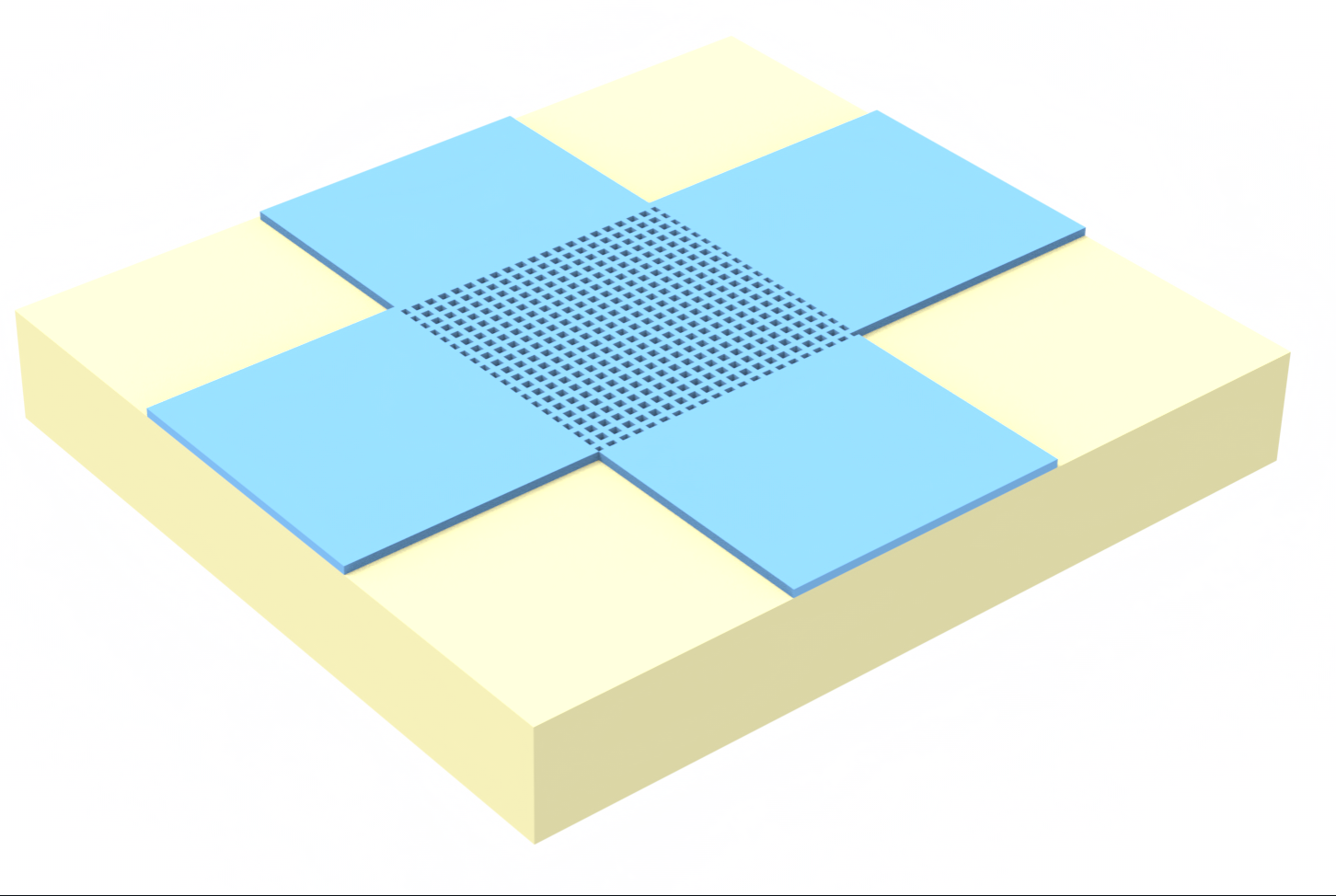
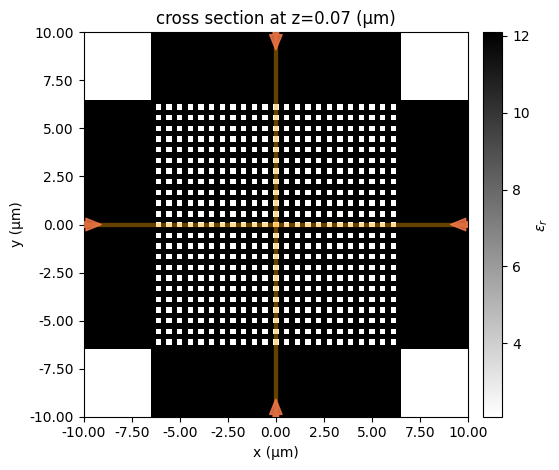
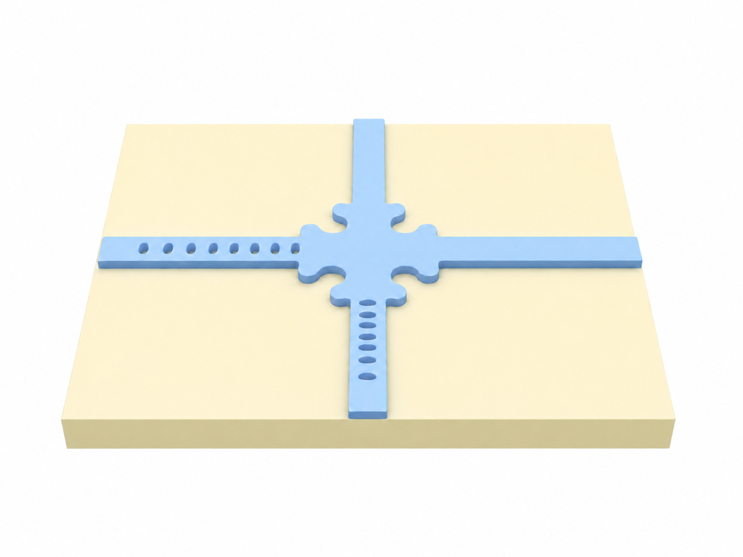
Here we model the quasi fundamental TE mode of orthogonal integrated waveguides with the horizontal and vertical polarization states with a normally incident centered free space beam. Using Tidy3D finite-difference time-domain (FDTD), simulations of electromagnetic waves incident on such a PSGC model the coupling to the four ports of the coupler as a function of polarization angle.
########################################## Import Libraries #########################################
#####################################################################################################

import numpy as np
import matplotlib.pyplot as plt

import tidy3d as td
from tidy3d import web
from tidy3d.plugins.mode import ModeSolver

#####################################################################################################
#####################################################################################################
13:25:03 EST WARNING: Configuration found in legacy location '~/.tidy3d'.
             Consider running 'tidy3d config migrate'.
Design Parameters
Define Global Parameters for the Simulation
####################################### Wavelength Parameters #######################################
#####################################################################################################

lda0 = 1.55                                                                                         # Central wavelength
freq0 = td.C_0 / lda0                                                                               # Central frequency
ldas = np.linspace(1.5, 1.6, 101)                                                                   # Wavelength range
freqs = td.C_0 / ldas                                                                               # Frequency range
fwidth = 0.5 * (np.max(freqs) - np.min(freqs))                                                      # Width of the source frequency range

######################################### Material Libraries ########################################
#####################################################################################################

si = td.material_library["cSi"]["Palik_Lossless"]                                                   # Load Silicon Library
sio2 = td.material_library["SiO2"]["Palik_Lossless"]                                                # Load Silicon Dioxide Library

######################################### Device Parameters #########################################
#####################################################################################################

w_wg = 13.0                                                                                         # Waveguide Width
t_wg = 0.22                                                                                         # Silicon Layer Thickness
l_wg = 5.0                                                                                          # I/O straight waveguide length

ff = 0.5                                                                                            # Grating Fill Factor
pitch = 0.556                                                                                       # Grating Pitch
Ng = 23                                                                                             # Number of Grating Periods

t_box  = 3.0                                                                                        # Buried Oxide Thickness
t_sub  = 1.0                                                                                        # Substrate Thickness (Arbitrary)
t_clad = 4.0                                                                                        # Cladding Thickness

t_etch = 0.07                                                                                       # Etch Depth
w_etch = ff*pitch                                                                                   # Etch Width

w0 = 5.2                                                                                            # Beam_Waist
theta = 0                                                                                           # Beam Angle 1
phi = 0                                                                                             # Beam Angle 2
pol_angle = 0                                                                                       # Polarization Angle (0 = Ex, np.pi = Ey)

inf_eff = 1000                                                                                      # Effective infinity

#####################################################################################################
#####################################################################################################

Lx = 2*l_wg+w_wg                                         # simulation domain size in x direction
Ly = 2*l_wg+w_wg                                         # simulation domain size in y direction
Lz = t_sub + t_clad + t_box + t_wg                       # simulation domain size in z direction
sim_size = (Lx, Ly, Lz)
Geometry
Define the Geometric Structure
######################################### Generate Geometry #########################################
#####################################################################################################

Substrate = td.Structure(
    geometry=td.Box.from_bounds(rmin=(-inf_eff, -inf_eff, -inf_eff),
                                rmax=(inf_eff, inf_eff, -t_wg/2 - t_box)),
    medium=si,
)

Buried_Ox = td.Structure(
    geometry=td.Box.from_bounds(rmin=(-inf_eff, -inf_eff, -t_wg/2 - t_box),
                                rmax=(inf_eff, inf_eff, -t_wg/2)),
    medium=sio2,
)

Cladding = td.Structure(
    geometry=td.Box.from_bounds(rmin=(-inf_eff, -inf_eff, -t_wg/2),
                                rmax=(inf_eff, inf_eff, t_wg/2 + t_clad + inf_eff)),
    medium=sio2,
)

Waveguide_Horz = td.Structure(
    geometry=td.Box.from_bounds(rmin=(-inf_eff, -w_wg/2, -t_wg/2),
                                rmax=(inf_eff, w_wg/2, t_wg/2)),
    medium=si,
)

Waveguide_Vert = td.Structure(
    geometry=td.Box.from_bounds(rmin=(-w_wg/2, -inf_eff, -t_wg/2),
                                rmax=(w_wg/2, inf_eff, t_wg/2)),
    medium=si,
)

PSGC = [Substrate, Buried_Ox, Cladding, Waveguide_Horz, Waveguide_Vert]

#####################################################################################################
#####################################################################################################

for i in range(Ng):
    for j in range(Ng):

        etch = td.Structure(
        geometry=td.Box.from_bounds(rmin=( (i-int((Ng-1)/2))*pitch - w_etch/2, (j-int((Ng-1)/2))*pitch - w_etch/2, t_wg/2-t_etch),
                                    rmax=( (i-int((Ng-1)/2))*pitch + w_etch/2, (j-int((Ng-1)/2))*pitch + w_etch/2, t_wg/2)),
        medium=sio2,
        )

        PSGC.append(etch)

#####################################################################################################
#####################################################################################################
Source, Monitors, and Meshing
Define a normally incident, centered gaussian beam source along with mode monitors at each of the ports of the PSGC. Field monitors are used to record cross sections of the simulated fields. Lastly a mesh override is defined over the full silicon layer.
########################################## Generate Source ##########################################
#####################################################################################################

pulse = td.GaussianPulse(freq0=freq0, fwidth=fwidth)

# Source definition
gauss_source = td.GaussianBeam(
  center=(0, 0, t_wg + 2),
  size=(Lx, Ly, 0),
  source_time=pulse,
  direction='-',
  pol_angle=pol_angle,
  angle_theta=theta,
  angle_phi=phi,
  waist_radius=w0,
  waist_distance=0,
  name="gauss_source",
)

########################################### Mode Monitors ###########################################
#####################################################################################################

mode_spec = td.ModeSpec(num_modes=5, target_neff=3.5, group_index_step = True, )

left = td.ModeMonitor(
    center=(-Lx/2 + 1, 0, t_wg/2),
    size=(0, w_wg + 5, 6 * t_wg),
    freqs=freqs,
    mode_spec=mode_spec,
    name="left",
)

right = td.ModeMonitor(
    center=(Lx/2 - 1, 0, t_wg/2),
    size=(0, w_wg + 5, 6 * t_wg),
    freqs=freqs,
    mode_spec=mode_spec,
    name="right",
)

top = td.ModeMonitor(
    center=(0, Ly/2 - 1, t_wg/2),
    size=(w_wg + 5, 0, 6 * t_wg),
    freqs=freqs,
    mode_spec=mode_spec,
    name="top",
)

bot = td.ModeMonitor(
    center=(0, -Ly/2 + 1, t_wg/2),
    size=(w_wg + 5, 0, 6 * t_wg),
    freqs=freqs,
    mode_spec=mode_spec,
    name="bot",
)

########################################### Field Monitors ##########################################
#####################################################################################################

XY_cross = td.FieldMonitor(
    center=(0, 0, t_wg/2), size=(td.inf, td.inf, 0), freqs=[freq0], name="XY_cross"
)

XZ_cross = td.FieldMonitor(
    center=(0, 0, t_wg/2), size=(td.inf, 0, td.inf), freqs=[freq0], name="XZ_cross"
)

YZ_cross = td.FieldMonitor(
    center=(0, 0, t_wg/2), size=(0, td.inf, td.inf), freqs=[freq0], name="YZ_cross"
)

############################################ Fine Meshing ###########################################
#####################################################################################################

override_gc = td.MeshOverrideStructure(
    name = 'override_gc',
    geometry = td.Box(center = [0, 0, 0], size = [td.inf, td.inf, 6*t_wg]),
    dl = [0.02, 0.02, 0.02],
)
Set Up Simulation
run_time = 2e-12  # simulation run time

# construct simulation
sim = td.Simulation(
    center=(0, 0, t_wg/2),
    size=sim_size,
    grid_spec = td.GridSpec(grid_x = td.AutoGrid(min_steps_per_wvl = 20, dl_min = 0), grid_y = td.AutoGrid(min_steps_per_wvl = 20, dl_min = 0), grid_z = td.AutoGrid(min_steps_per_wvl = 20, dl_min = 0), wavelength = lda0, override_structures = [override_gc], ),
    structures=PSGC,
    sources=[gauss_source],
    monitors=[left, right, top, bot, XY_cross, XZ_cross, YZ_cross],
    run_time=run_time,
    version = '2.10.0',
    subpixel = td.SubpixelSpec(pec = td.PECConformal(), ),
    medium=sio2,
)
sim.plot_eps(z = t_wg/2 - t_etch/2, freq=freq0, vlim = (-10, 10), hlim = (-10, 10))
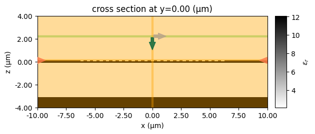
sim.plot_eps(y=0, freq=freq0, vlim = (-4, 4), hlim = (-10, 10))
plt.show()
13:25:04 EST WARNING: More than 200 structures use the same medium. For
             performance, use a 'GeometryGroup' or boolean operations to combine
             geometries that share a medium.
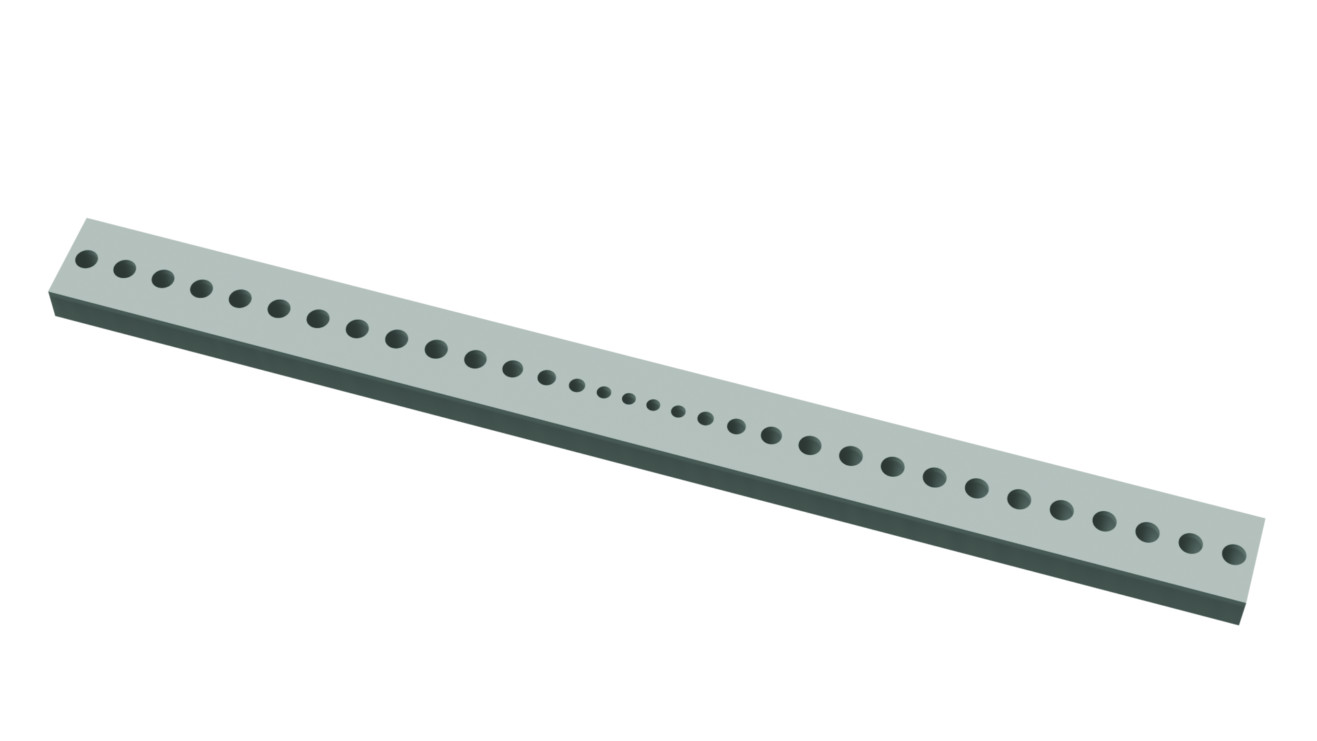
sim.plot_3d()
Modal Analysis
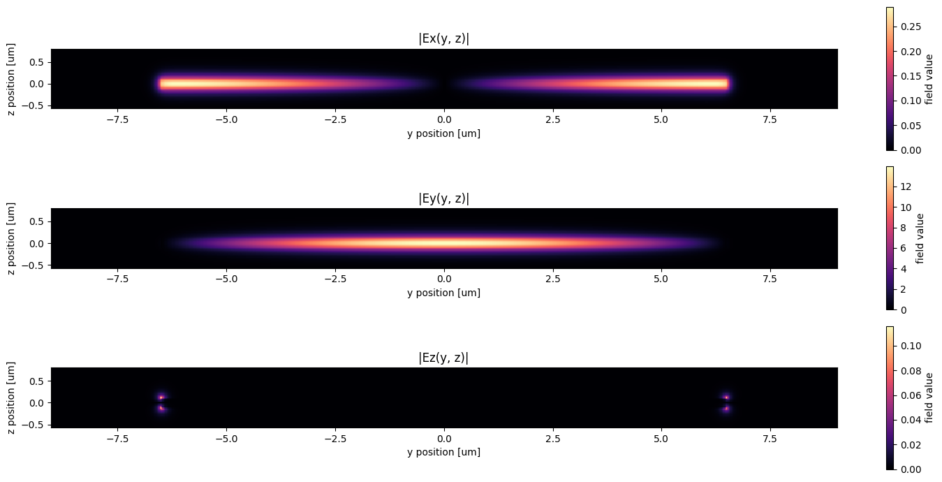
Simulate the mode profiles at each of the output ports to determine the fundamental mode index.
mode_spec = td.ModeSpec(num_modes=5, target_neff=3.5, group_index_step = True, )

mode_solver = ModeSolver(
    simulation=sim,
    plane=td.Box(center=left.center, size=left.size),
    mode_spec=mode_spec,
    freqs=[freq0],
)
mode_data = mode_solver.solve()
13:25:05 EST WARNING: Use the remote mode solver with subpixel averaging for
             better accuracy through 'tidy3d.web.run(...)' or the deprecated
             'tidy3d.plugins.mode.web.run(...)'.
Plot Modes
mode_idx = 0
f, (ax1, ax2, ax3) = plt.subplots(3, 1, tight_layout=True, figsize=(15, 7))
abs(mode_data.Ex.isel(mode_index=mode_idx)).plot(x="y", y="z", ax=ax1, cmap="magma")
abs(mode_data.Ey.isel(mode_index=mode_idx)).plot(x="y", y="z", ax=ax2, cmap="magma")
abs(mode_data.Ez.isel(mode_index=mode_idx)).plot(x="y", y="z", ax=ax3, cmap="magma")

ax1.set_title("|Ex(y, z)|")
ax1.set_aspect("equal")
ax2.set_title("|Ey(y, z)|")
ax2.set_aspect("equal")
ax3.set_title("|Ez(y, z)|")
ax3.set_aspect("equal")
plt.show()
Define Job and Estimate Cost
job = web.Job(simulation=sim, task_name="PSGC", verbose=True)
estimated_cost = web.estimate_cost(job.task_id)
13:25:18 EST Created task 'PSGC' with resource_id
             'fdve-2744f6c2-0dbe-4758-9dea-3db64168985d' and task_type 'FDTD'.
             View task using web UI at
             'https://tidy3d.simulation.cloud/workbench?taskId=fdve-2744f6c2-0db
             e-4758-9dea-3db64168985d'.
Task folder: 'default'.
Output()
13:25:25 EST Estimated FlexCredit cost: 12.539. Minimum cost depends on task
             execution details. Use 'web.real_cost(task_id)' to get the billed
             FlexCredit cost after a simulation run.
13:25:29 EST Estimated FlexCredit cost: 12.539. Minimum cost depends on task
             execution details. Use 'web.real_cost(task_id)' to get the billed
             FlexCredit cost after a simulation run.
Run Job and Record Data (Approximately 5 credits)
sim_data = job.run(path="data_TM/simulation_data.hdf5")
13:25:32 EST status = success
Output()
13:26:09 EST Loading simulation from data_TM/simulation_data.hdf5
13:26:10 EST WARNING: More than 200 structures use the same medium. For
             performance, use a 'GeometryGroup' or boolean operations to combine
             geometries that share a medium.
             WARNING: Warning messages were found in the solver log. For more
             information, check 'SimulationData.log' or use
             'web.download_log(task_id)'.
Plot Field Cross Sections
f1 = plt.figure(figsize=(15,6))
ax = f1.add_subplot(1,1,1)
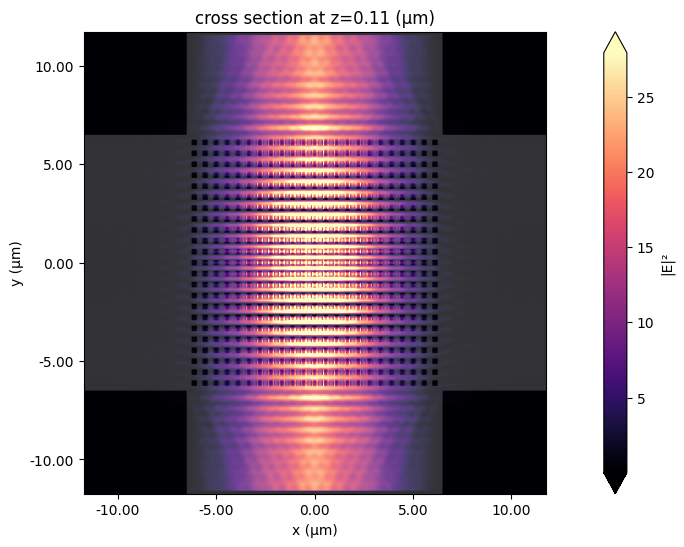
sim_data.plot_field(
    field_monitor_name="XY_cross", field_name="E", val="abs^2", f=freq0, ax=ax)
plt.show()


f1 = plt.figure(figsize=(15,6))
ax = f1.add_subplot(1,1,1)
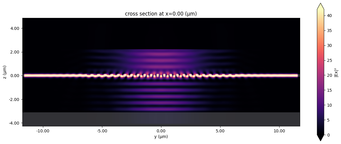
sim_data.plot_field(
    # field_monitor_name="XZ_cross", field_name="Ey", val="real", f=freq0, ax=ax)
    field_monitor_name="YZ_cross", field_name="Ex", val="abs^2", f=freq0, ax=ax)
plt.show()
PSGC Efficiency
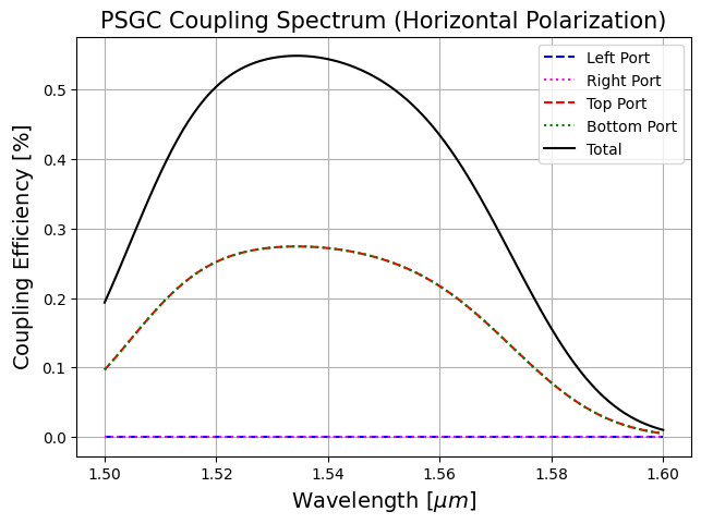
amp_left = sim_data["left"].amps.sel(mode_index=0, direction="-")
T_left = np.abs(amp_left) ** 2

amp_right = sim_data["right"].amps.sel(mode_index=0, direction="+")
T_right = np.abs(amp_right) ** 2

amp_top = sim_data["top"].amps.sel(mode_index=0, direction="+")
T_top = np.abs(amp_top) ** 2

amp_bot = sim_data["bot"].amps.sel(mode_index=0, direction="-")
T_bot = np.abs(amp_bot) ** 2

f1 = plt.figure(figsize=(16,5))
ax = f1.add_subplot(1,2,1)

ax.plot(ldas, T_left, linestyle = 'dashed', color= 'blue')
ax.plot(ldas, T_right, linestyle = 'dotted', color= 'magenta')
ax.plot(ldas, T_top, linestyle = 'dashed', color= 'red')
ax.plot(ldas, T_bot, linestyle = 'dotted', color= 'green')
ax.plot(ldas, T_bot + T_top + T_right + T_left, 'black')

ax.grid()
ax.set_xlabel('Wavelength [$\mu{m}$]', fontsize = 14)
ax.set_ylabel('Coupling Efficiency [$\%$]', fontsize = 14)
ax.set_title('PSGC Coupling Spectrum (Horizontal Polarization)', fontsize = 15)

ax.legend(['Left Port', 'Right Port', 'Top Port', 'Bottom Port', 'Total'], fontsize = 10)
plt.show()


 TERMS & CONDITIONS


 How the process works:
 Try this real URL to see an example: