





from __future__ import annotations

import matplotlib.pyplot as plt
import numpy as np
import tidy3d as td
import tidy3d.web as web
from tidy3d.plugins.mode import ModeSolver

td.config.logging.level = "ERROR"
TIDY3D
LEARNING CENTER
Example Library

EME convergence for a bent anisotropic waveguide (LiNbO₃)
Lithium niobate (LiNbO₃) is a key material in integrated photonics due to its large electro-optic coefficient and wide transparency window. However, it is a uniaxial crystal: its permittivity is described by a tensor, not a scalar. This has important consequences when the waveguide is bent.
In this notebook we:
- Run an FDTD simulation of a 180° LiNbO₃ waveguide bend to obtain a reference transmittance.
- Run EME simulations of the same bend with increasing numbers of cells.
- Show that a single EME cell overestimates transmission and explain the physical origin.
- Demonstrate convergence of EME to the FDTD result as the cell count increases.
For an introduction to the EME solver in Tidy3D see the EME solver tutorial and the bent waveguides with EME notebook.
Physics Background: Why Anisotropy Complicates Bent-Waveguide EME
The Rotating Permittivity Tensor
LiNbO₃ is uniaxial: it has one extraordinary index \(n_e \approx 2.14\) along the optic (c) axis and an ordinary index \(n_o \approx 2.21\) along the other two directions (at 1.55 µm). In the material API, Zelmon1997(1) places the extraordinary axis along the global \(y\) direction (index 2 would place it along \(z\)). The lab-frame tensor used here is therefore
\[ \varepsilon_\text{lab} = \begin{pmatrix} n_o^2 & 0 & 0 \\ 0 & n_e^2 & 0 \\ 0 & 0 & n_o^2 \end{pmatrix} \qquad \text{(optic axis along } y\text{)} . \]
The key point is that the optic axis lies in the plane of the bend (the \(x\)–\(y\) plane). In a straight waveguide propagating along \(x\) the tensor is constant — modes are quasi-TE / quasi-TM and propagate without cross-coupling. However, in a bent waveguide (ring in the \(x\)–\(y\) plane) the local propagation direction rotates by an angle \(\phi\) as the wave travels around the bend. From the co-moving frame the effective tensor becomes
\[ \varepsilon_\text{local}(\phi) = R_z(\phi)^\top \, \varepsilon_\text{lab} \, R_z(\phi) . \]
Because the optic axis lies in the rotation (\(x\)–\(y\)) plane and \(n_o \neq n_e\), this rotation produces off-diagonal terms that grow with \(\phi\). The local eigenmodes therefore evolve continuously as the wave travels — the quasi-TE and quasi-TM modes of the bent waveguide mix along the propagation path.
Consequence for EME
EME divides the waveguide into \(N\) cells and matches eigenmodes at each cell boundary. At every interface the two adjacent mode bases are slightly misaligned due to the incremental tensor rotation — generating partial back-reflections and mode conversion.
| EME cells | Physical picture |
|---|---|
| 1 | Entire 180° bend is one uniform section. No inter-cell interfaces → no reflections from tensor rotation → transmission is overestimated. |
| few | Tensor rotation is approximated as a staircase; dominant back-reflection is captured. |
| many | Staircase finely resolves the continuous rotation → converges to FDTD. |
The loss mechanism is not geometric bending loss (negligible at \(r = 5\) µm for this waveguide) but polarization-state evolution driven by the rotating anisotropy.
# ── Simulation parameters ──────────────────────────────────────────────────
wavelength = 1.55  # free-space wavelength (µm)
freq0 = td.C_0 / wavelength

radius = 5.0  # bend radius (µm)
width = 0.6  # waveguide width (µm)
thickness = 0.4  # waveguide thickness (µm)

num_modes = 5  # number of modes in mode solvers
target_neff = 1.65  # target effective index for mode search
plane_size = (9.0, 9.0)  # cross-section window size (µm)
min_steps_per_wvl = 30  # grid resolution (steps per wavelength)

# ── Materials ───────────────────────────────────────────────────────────────
SiO2 = td.material_library["SiO2"]["Palik_Lossless"]
# (1): extraordinary (optic) axis along global y — in the bend plane, the
# orientation-sensitive case. Use (2) to place the optic axis along z instead.
LiNbO3 = td.material_library["LiNbO3"]["Zelmon1997"](1)
Step 1 — FDTD Reference Simulation
We model the 180° bend as a full ring in the FDTD simulation:
- Geometry: outer Cylinder minus inner cylinder (LiNbO₃ annulus on SiO₂).
-
Source: ModeSource at the bottom of the ring
(0, −r, 0), launching in the +x direction with a negative bend radius (the center of curvature is on the +y side of the source). -
Monitor: ModeMonitor at the top of the ring
(0, +r, 0), measuring the amplitudes of all guided modes travelling in the −x direction (i.e., those that have propagated 180° around the bend). - Boundaries: Absorber on ±x to suppress re-entry of any radiation that escapes the open side of the ring; PML on ±y, ±z.
The bend curvature is encoded in the ModeSpec via bend_radius and bend_axis.
The source and monitor sort their modes with ModeSortSpec(sort_key="fill_fraction_box", bounding_box=core_box): in a bent, anisotropic waveguide the default ordering (by effective index) does not reliably put the guided fundamental first, so we instead rank modes by the fraction of their intensity that falls inside a box wrapping the core. The most core-confined (guided) mode then lands at mode_index = 0 regardless of polarization or tensor-rotation mixing. (fill_fraction_box ranks by confinement, not polarization — the polarization is verified separately.)
def build_fdtd_bend(
    radius=5.0,
    width=0.6,
    thickness=0.4,
    num_modes=10,
    target_neff=1.65,
    freq0=td.C_0 / 1.55,
    core_medium=LiNbO3,
    background_medium=SiO2,
    plane_size=(9.0, 9.0),
    min_steps_per_wvl=30,
    mode_index=0,
):
    """Build an FDTD simulation of a 180-degree LiNbO3 waveguide bend.

    The geometry is a ring (annular cylinder) with a ModeSource at the
    bottom and a ModeMonitor at the top, measuring 180-degree transmission.
    """
    wavelength = td.C_0 / freq0
    cross_sec = (0, plane_size[0], plane_size[1])  # cross-section for mode planes

    core_box_src = td.Box(center=(0, -radius, 0), size=(0, width, thickness))
    core_box_mon = td.Box(center=(0, radius, 0), size=(0, width, thickness))

    sort_spec_src = td.ModeSortSpec(sort_key="fill_fraction_box", bounding_box=core_box_src)
    sort_spec_mon = td.ModeSortSpec(sort_key="fill_fraction_box", bounding_box=core_box_mon)

    # Bend mode specs
    # Source at bottom (0, -r, 0) going in +x: center of curvature is at +y → negative radius
    # Monitor at top  (0, +r, 0) receiving in -x: center of curvature is at -y → positive radius
    mode_spec_src = td.ModeSpec(
        num_modes=num_modes,
        target_neff=target_neff,
        bend_radius=-radius,
        bend_axis=1,
        num_pml=(12, 12),
        sort_spec=sort_spec_src,
        precision="double",
    )
    mode_spec_mon = td.ModeSpec(
        num_modes=num_modes,
        target_neff=target_neff,
        bend_radius=radius,
        bend_axis=1,
        num_pml=(12, 12),
        sort_spec=sort_spec_mon,
        precision="double",
    )

    # Ring geometry: outer cylinder minus inner cylinder
    outer = td.Cylinder(center=(0, 0, 0), radius=radius + width / 2, length=thickness, axis=2)
    inner = td.Cylinder(center=(0, 0, 0), radius=radius - width / 2, length=thickness, axis=2)
    ring = td.Structure(geometry=outer - inner, medium=core_medium)

    # Simulation domain — asymmetric: source side open, far side has extra room
    ring_outer = radius + width / 2
    x_min, x_max = -wavelength, ring_outer + 2 * wavelength
    sim_size = (x_max - x_min, 2 * (radius + width + 2 * wavelength), plane_size[1])
    sim_center = ((x_min + x_max) / 2, 0, 0)

    source = td.ModeSource(
        center=(0, -radius, 0),
        size=cross_sec,
        source_time=td.GaussianPulse(freq0=freq0, fwidth=0.1 * freq0),
        mode_spec=mode_spec_src,
        direction="+",
        mode_index=mode_index,
    )

    # Field monitor in the z=0 plane for visualization
    field_xy = td.FieldMonitor(
        center=(0, 0, 0),
        size=(td.inf, td.inf, 0),
        freqs=[freq0],
        name="field_xy",
    )

    # Mode amplitude monitor at the output (top of the ring)
    mode_out = td.ModeMonitor(
        center=(0, radius, 0),
        size=cross_sec,
        freqs=[freq0],
        name="mode_out",
        mode_spec=mode_spec_mon,
    )

    return td.Simulation(
        size=sim_size,
        center=sim_center,
        structures=[ring],
        sources=[source],
        monitors=[field_xy, mode_out],
        medium=background_medium,
        grid_spec=td.GridSpec.auto(min_steps_per_wvl=min_steps_per_wvl),
        run_time=0.6e-12,
        boundary_spec=td.BoundarySpec(
            x=td.Boundary.absorber(num_layers=160),
            y=td.Boundary.pml(),
            z=td.Boundary.pml(),
        ),
    )
fdtd_sim_test = build_fdtd_bend(
radius=radius,
width=width,
thickness=thickness,
num_modes=num_modes,
target_neff=target_neff,
freq0=freq0,
plane_size=plane_size,
min_steps_per_wvl=min_steps_per_wvl,
mode_index=0, # fundamental quasi-TE bend mode
)
fig, ax = plt.subplots(figsize=(6, 6))
fdtd_sim_test.plot(z=0, ax=ax)
ax.set_title("FDTD simulation — z = 0 cross-section")
plt.tight_layout()
plt.show()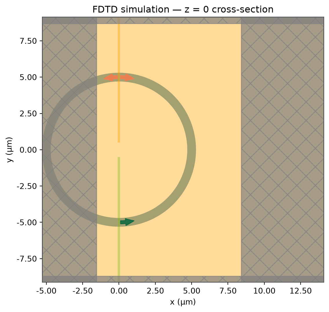
Mode Solver Verification
Before running the FDTD, we use the ModeSolver plugin on the source plane to confirm that the fundamental bend mode is the one being excited.
ms = ModeSolver(
    simulation=fdtd_sim_test,
    mode_spec=fdtd_sim_test.sources[0].mode_spec,
    plane=fdtd_sim_test.sources[0].geometry,
    freqs=fdtd_sim_test.sources[0].source_time.freq0,
)

ms_data = web.run(ms)
01:03:18 UTC Created task 'mode_solver_2026-07-11_01-03-18' with resource_id 'mo-fa081187-bfa6-47ed-a9b3-c2bac0b3fbcd' and task_type 'MODE_SOLVER'.
             View task using web UI at
             'https://tidy3d.simulation.cloud/workbench?taskId=mo-fa081187-bfa6-
             47ed-a9b3-c2bac0b3fbcd'.
Task folder: 'default'.
01:03:20 UTC Estimated FlexCredit cost: 0.013. For this solver type, the
             estimate is the final billed cost.
01:03:21 UTC status = success
01:03:24 UTC Loading results from simulation_data.hdf5
Next, we can check the respective TE and TM fundamental modes.
df = ms_data.to_dataframe()
df["Fill factor (%)"] = ms_data.fill_fraction_box.values.squeeze() * 100
df.head(10)| wavelength | n eff | k eff | loss (dB/cm) | TE (Ey) fraction | wg TE fraction | wg TM fraction | mode area | Fill factor (%) | ||
|---|---|---|---|---|---|---|---|---|---|---|
| f | mode_index | |||||||||
| 1.934145e+14 | 0 | 1.55 | 1.652945 | 0.007050 | 2482.247210 | 0.986371 | 0.847809 | 0.906344 | 1.268877 | 32.268825 |
| 1 | 1.55 | 1.630062 | 0.009250 | 3256.907542 | 0.013816 | 0.879321 | 0.873460 | 1.622651 | 22.946851 | |
| 2 | 1.55 | 1.713282 | 0.143217 | 50426.404124 | 0.006008 | 0.991446 | 0.593760 | 16.523307 | 0.007609 | |
| 3 | 1.55 | 1.671566 | 0.157827 | 55570.272482 | 0.023067 | 0.968163 | 0.591092 | 18.798184 | 0.005693 | |
| 4 | 1.55 | 1.696173 | 0.148796 | 52390.513163 | 0.012374 | 0.980756 | 0.593797 | 18.468442 | 0.000130 |
# Side-by-side view of the two most-confined modes (mode_index = 0 and 1).
# TE_fraction tells us which one is quasi-TE (horizontal E in the waveguide
# plane, dominant Ey) and which is quasi-TM (vertical E, dominant Ez).
te_frac = ms_data.TE_fraction.isel(f=0).values  # shape: (num_modes,)

fig, axes = plt.subplots(1, 2, figsize=(11, 4))
for ax, m in zip(axes, [0, 1]):
    label = "quasi-TE" if te_frac[m] > 0.5 else "quasi-TM"
    component = "Ey" if te_frac[m] > 0.5 else "Ez"  # dominant transverse E
    ms.plot_field(component, "real", mode_index=m, ax=ax)
    ax.set_title(f"mode {m} — {label}  (TE frac = {te_frac[m]:.2f}) — {component}")

plt.tight_layout()
plt.show()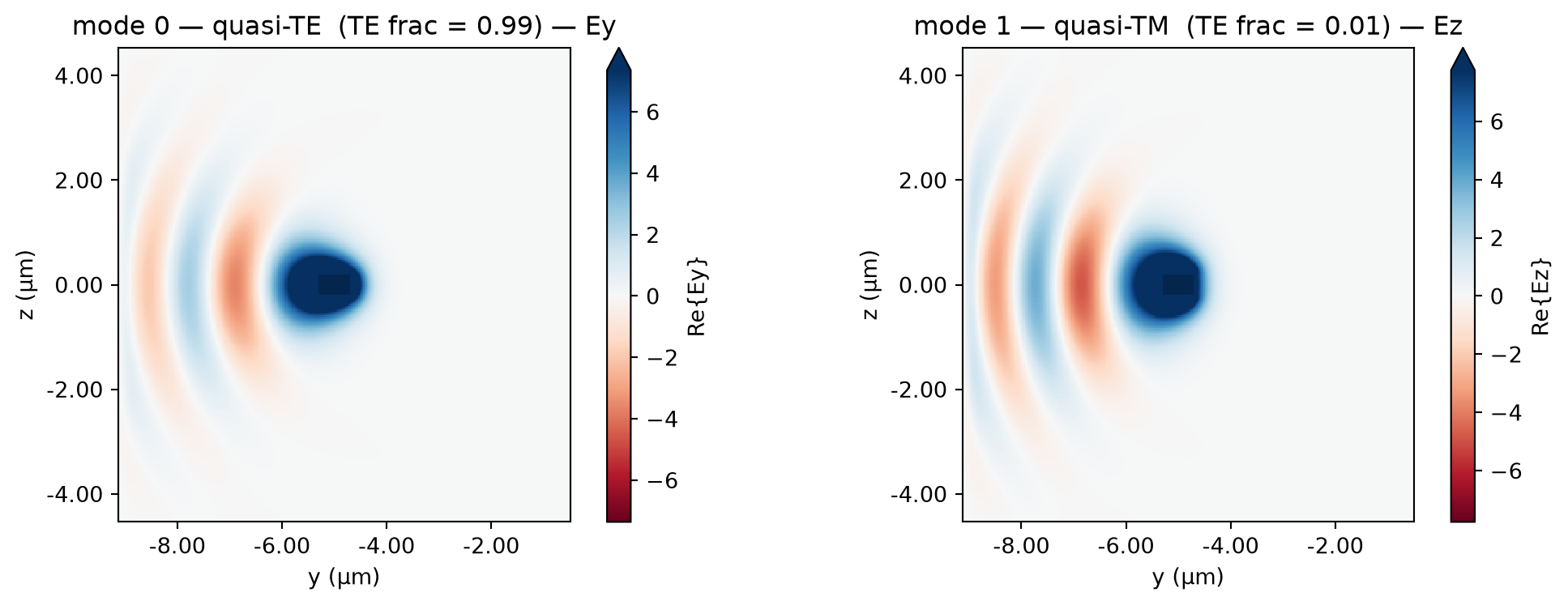
mode_index = 0
print("Selected mode index:", mode_index)
Selected mode index: 0fdtd_sim = build_fdtd_bend(
radius=radius,
width=width,
thickness=thickness,
num_modes=num_modes,
target_neff=target_neff,
freq0=freq0,
plane_size=plane_size,
min_steps_per_wvl=min_steps_per_wvl,
mode_index=mode_index, # fundamental quasi-TE bend mode
)
fdtd_data = web.run(
fdtd_sim,
task_name="bent_LiNbO3_FDTD",
path="FDTD_GT.hdf5",
)01:03:26 UTC Created task 'bent_LiNbO3_FDTD' with resource_id 'fdve-2c414ee8-f36d-4b4f-9ffe-302e436edd64' and task_type 'FDTD'.
             View task using web UI at
             'https://tidy3d.simulation.cloud/workbench?taskId=fdve-2c414ee8-f36
             d-4b4f-9ffe-302e436edd64'.
Task folder: 'default'.
01:03:27 UTC Estimated FlexCredit cost: 1.355. This assumes the FDTD solver runs
             for the full simulation time; if early shutoff is reached, the
             billed cost can be lower. Use 'web.real_cost(task_id)' to get the
             billed FlexCredit cost after a simulation run.
01:03:28 UTC status = success
01:03:31 UTC Loading results from FDTD_GT.hdf5
# Transmittance into the fundamental guided mode at the output (|S21(0,0)|²).
amps_out = fdtd_data["mode_out"].amps.sel(direction="-")
T_fdtd = float(np.abs(amps_out.isel(f=0, mode_index=mode_index)) ** 2)
print(f"FDTD transmittance: T = {T_fdtd:.4f}  ({10 * np.log10(T_fdtd):.2f} dB)")

# Field plot
fig, ax = plt.subplots(figsize=(7, 6))
fdtd_data.plot_field("field_xy", "Ey", "real", ax=ax)
ax.set_title("FDTD — Ey (real) at z = 0")
plt.tight_layout()
plt.show()
FDTD transmittance: T = 0.4948 (-3.06 dB)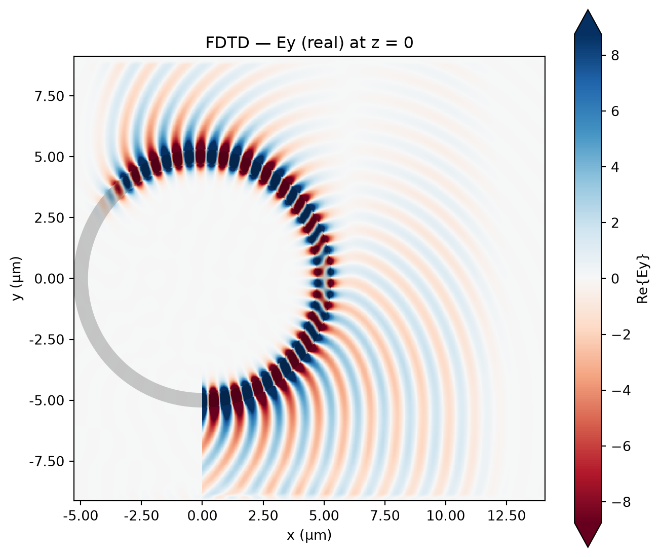
Step 2 — EME Convergence Study
EME Setup for a Bent Waveguide
In Tidy3D’s EMESimulation, a bent waveguide is modelled as a straight simulation box whose length matches the bend arc length (\(L = \pi r\) for a 180° bend). In each EME cell, bend_radius is specified in EMEModeSpec to compute the correct curved eigenmodes via conformal mapping (bend boundary conditions). We set precision="double" because, in single precision, the near-degenerate quasi-TE and quasi-TM modes of this anisotropic bend can be mis-sorted, which affects the convergence. The longitudinal discretization is controlled by EMEUniformGrid.
When the waveguide medium is isotropic, the curved eigenmodes are the same regardless of where along the arc the cross-section is taken — one EME cell is sufficient.
When the medium is anisotropic (LiNbO₃), the lab-frame permittivity tensor projects differently onto the local propagation frame at each position \(\phi\) along the arc. Dividing the bend into \(N\) cells with independently computed eigenmodes causes \(N-1\) inter-cell interfaces at which mode-matching generates back-reflected amplitudes.
On
bend_medium_frame. This example relies onbend_medium_frame="global"— the default inEMEModeSpecsince Tidy3D 2.11 — which keeps the LiNbO₃ crystal axes fixed in physical space, the same convention as FDTD. Before this option existed (and as in many other EME solvers) the effective behavior was"co_rotating", where the medium bends together with the local cross-section; in that frame the tensor is identical in every cell, so you would obtain the single-cell (\(N=1\)) result regardless of the number of cells, and the convergence effect studied here would not appear.
Expected Behavior
- \(N = 1\): No interfaces → no back-scattering from tensor rotation → overestimated transmission.
- Increasing \(N\): Each added interface captures more of the physical mode conversion → transmission moves toward the FDTD reference.
- Large \(N\): EME converges toward FDTD. Note that a piecewise-constant EME approximation to a smoothly rotating anisotropic tensor is not guaranteed to make \(|S_{00}|^2\) decrease strictly monotonically — modal truncation and mode reordering/conversion can produce small non-monotonic wiggles. Convergence is therefore best judged with a mode-count sweep and the interface residual diagnostics (below), rather than by strict monotonicity of \(|S_{00}|^2\) alone.
We sweep \(N \in \{1, 2, 3, 4, 5\}\) and compare with \(T_\text{FDTD}\).
def build_eme_bend(fdtd_sim, num_cells):
    """Build an EME bend simulation derived from an existing FDTD simulation.

    All parameters (radius, width, thickness, num_modes, target_neff, freq0,
    plane size, and materials) are extracted from fdtd_sim, guaranteeing that
    both simulations model the exact same structure.

    Parameters
    ----------
    fdtd_sim : td.Simulation
        The FDTD bend simulation returned by build_fdtd_bend().
    num_cells : int
        Number of uniform EME cells to divide the 180-degree arc into.
    """
    src = fdtd_sim.sources[0]
    ring_geom = fdtd_sim.structures[0].geometry  # ClipOperation: outer - inner

    # ── Extract all parameters from the FDTD simulation ────────────────────
    freq0 = src.source_time.freq0
    num_modes = src.mode_spec.num_modes
    target_neff = src.mode_spec.target_neff
    radius = abs(src.mode_spec.bend_radius)  # stored as negative in the source
    plane_size = (src.size[1], src.size[2])
    num_pml = src.mode_spec.num_pml
    grid_spec = fdtd_sim.grid_spec

    core_medium = fdtd_sim.structures[0].medium
    background_medium = fdtd_sim.medium

    # Width and thickness from the ring geometry (outer Cylinder - inner Cylinder)
    outer_cyl = ring_geom.geometry_a
    inner_cyl = ring_geom.geometry_b
    width = outer_cyl.radius - inner_cyl.radius
    thickness = outer_cyl.length
    # ───────────────────────────────────────────────────────────────────────

    arc_length = np.pi * radius  # 180-degree arc

    # Sort modes by fill_fraction_box so the well-confined guided mode sits at
    # index 0 at every EME cell boundary. Each cell boundary is a plane normal
    # to x at a different x, so the bounding_box needs to span all of them —
    # use td.inf along x (core centred at y = 0, z = 0 since the EME models a
    # straight waveguide with curvature encoded in bend_radius).
    core_box_eme = td.Box(center=(0, 0, 0), size=(td.inf, width, thickness))
    mode_spec = td.EMEModeSpec(
        num_modes=num_modes,
        target_neff=target_neff,
        bend_radius=radius,
        bend_axis=1,
        num_pml=num_pml,
        increasing_mode_tolerance=1e-3,
        sort_spec=td.ModeSortSpec(sort_key="fill_fraction_box", bounding_box=core_box_eme),
        precision="double",
    )

    # Infinite straight waveguide slab (curvature fully encoded in mode_spec)
    wg = td.Structure(
        geometry=td.PolySlab(
            axis=2,
            slab_bounds=(-thickness / 2, thickness / 2),
            vertices=[
                [-1e15, -width / 2],
                [-1e15, width / 2],
                [1e15, width / 2],
                [1e15, -width / 2],
            ],
        ),
        medium=core_medium,
    )

    return td.EMESimulation(
        size=(arc_length, plane_size[0], plane_size[1]),
        center=(0, 0, 0),
        structures=[wg],
        medium=background_medium,
        axis=0,
        freqs=[freq0],
        eme_grid_spec=td.EMEUniformGrid(num_cells=num_cells, mode_spec=mode_spec),
        grid_spec=grid_spec,
    )
num_cells_list = [1, 2, 3, 4, 5]
eme_sims = [build_eme_bend(fdtd_sim, num_cells=n) for n in num_cells_list]
eme_batch = {f"bent_LiNbO3_EME_N{n:02d}": sim for n, sim in zip(num_cells_list, eme_sims)}
eme_results = web.run(eme_batch)
eme_data_list = [eme_results[f"bent_LiNbO3_EME_N{n:02d}"] for n in num_cells_list]01:03:36 UTC Started working on Batch containing 5 tasks.
01:03:41 UTC Maximum FlexCredit cost: 0.194 for the whole batch.
             Use 'Batch.real_cost()' to get the billed FlexCredit cost after
             completion.
01:03:43 UTC Batch complete.
# S00 is the fundamental-to-fundamental transmission. fill_fraction_box sorts the
# most core-confined mode to index 0, but not by polarization — so here we also
# confirm the index-0 port mode is the quasi-TE fundamental: effective index
# n_eff ~ 1.65 and TE fraction ~ 1, i.e. S00 really is the quasi-TE -> quasi-TE
# channel. (A per-cell check follows below.)
T_eme = []
for n, eme_data in zip(num_cells_list, eme_data_list):
    T = float(eme_data.smatrix.S21.isel(mode_index_in=0, mode_index_out=0, f=0).abs.item() ** 2)
    # Effective index and TE fraction of the index-0 port mode (n_eff averaged
    # over the 2 ports; TE fraction = |Ey|^2 / (|Ey|^2 + |Ez|^2), worst of the 2).
    pm = eme_data.port_modes
    neff0 = float(pm.n_complex.real.isel(mode_index=0).mean().values)
    Ey2 = (abs(pm.Ey) ** 2).sum(("x", "y", "z"))
    Ez2 = (abs(pm.Ez) ** 2).sum(("x", "y", "z"))
    te0 = float((Ey2 / (Ey2 + Ez2)).real.isel(mode_index=0).min().values)
    print(
        f"  N = {n:2d} cells  \u2192  T = {T:.4f}  ({10 * np.log10(T):.2f} dB)   |  mode-0: n_eff \u2248 {neff0:.4f}, TE fraction \u2265 {te0:.3f}"
    )
    T_eme.append(T)
N = 1 cells → T = 0.6123 (-2.13 dB) | mode-0: n_eff ≈ 1.6835, TE fraction ≥ 0.984
N = 2 cells → T = 0.5108 (-2.92 dB) | mode-0: n_eff ≈ 1.6661, TE fraction ≥ 0.986
N = 3 cells → T = 0.5023 (-2.99 dB) | mode-0: n_eff ≈ 1.6572, TE fraction ≥ 0.987
N = 4 cells → T = 0.5016 (-3.00 dB) | mode-0: n_eff ≈ 1.6535, TE fraction ≥ 0.987
N = 5 cells → T = 0.5017 (-3.00 dB) | mode-0: n_eff ≈ 1.6517, TE fraction ≥ 0.987fig, ax = plt.subplots(figsize=(7, 4))
ax.plot(
num_cells_list,
T_eme,
"o-",
color="steelblue",
linewidth=1.8,
markersize=7,
label="EME",
)
ax.axhline(
T_fdtd,
color="crimson",
linestyle="--",
linewidth=1.6,
label=f"FDTD reference (T = {T_fdtd:.3f})",
)
ax.set_xlabel("Number of EME cells", fontsize=12)
ax.set_ylabel("Transmittance", fontsize=12)
ax.set_title("EME convergence — 180° LiNbO₃ bend (r = 5 µm, λ = 1.55 µm)", fontsize=12)
ax.legend(fontsize=11)
ax.set_xlim(0, max(num_cells_list) + 1)
ax.grid(True, alpha=0.3)
plt.tight_layout()
plt.show()
print(f"\nN={num_cells_list[0]} overestimates by {(T_eme[0] - T_fdtd) / T_fdtd * 100:.1f}%")
print(f"N={num_cells_list[-2]} error vs FDTD: {abs(T_eme[-2] - T_fdtd) / T_fdtd * 100:.1f}%")
print(f"N={num_cells_list[-1]} error vs FDTD: {abs(T_eme[-1] - T_fdtd) / T_fdtd * 100:.1f}%")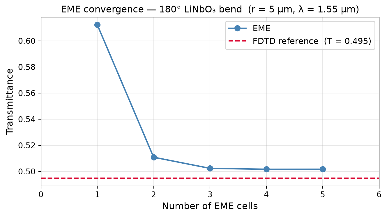
N=1   overestimates by  23.8%
N=4 error vs FDTD:    1.4%
N=5 error vs FDTD:    1.4%
Discussion
Behavior with Cell Count
The plot shows three regimes:
| Region | Cells | Observation |
|---|---|---|
| Single-cell | \(N = 1\) | T ≈ 0.61 — large overestimate (~24% above FDTD). |
| Transition | \(N = 2\) | T drops sharply as the dominant back-reflection is captured. |
| Stable | \(N \geq 3\) | T ≈ 0.50, approaching FDTD to within ~2%. |
Why One Cell Is Not Enough
With a single EME cell the solver computes one set of curved eigenmodes for the entire 180° arc, assuming a fixed tensor orientation. At the ports, these modes are matched to straight-waveguide modes. With no internal interfaces, the system behaves close to a lossless propagator.
In reality, the eigenmodes evolve continuously as the tensor rotates. Splitting the arc into \(N\) cells approximates this as discrete steps. At each step, modes are reprojected onto a new basis, introducing reflections and mode mismatch. Increasing \(N\) improves this approximation.
Convergence Diagnostics (N = 5 cells)
The cell-count curve is only meaningful if, at each cell count, the result is already converged in the number of expansion modes, and if the mode tracked at index 0 is really the intended quasi-TE fundamental. For the converged N = 5 case we therefore:
-
sweep the number of modes with
EMEModeSweep(free; the modes are solved once and reused); - inspect the mode identity (effective index and TE fraction) at every cell, recorded with an
EMEModeSolverMonitor; - check the interface field residual from
eme_diagnosticsas a convergence criterion.
What eme_diagnostics reports
EME builds the scattering matrix by enforcing continuity of the tangential E and H fields at every cell interface, expressed in a truncated set of modes. If that basis is too small, the matched fields do not quite agree across the interface, so the leftover mismatch is the interface residual. Setting eme_diagnostics=True makes the solver compute and store, per interface and per swept mode count:
-
normalized_tangential_E_residual/normalized_tangential_H_residual— the incident-normalized squared tangential-field mismatch over the whole cross-section; -
normalized_aperture_tangential_E_residual/normalized_aperture_tangential_H_residual— the same, but restricted to the physical aperture, excluding the PML, so the metric is not masked by PML absorption; -
power_defect— the violation of power conservation at the interface.
A well-converged expansion reproduces the interface fields almost exactly, so the residual decreases toward zero (and plateaus) as modes are added. This is a direct, physical convergence check: unlike \(|S_{00}|^2\), it does not require strict monotonicity and is not fooled by mode reordering. Below we plot the non-PML tangential-E residual of the incident fundamental mode (worst case over interfaces and ports) versus the mode count. (High-order radiative / PML-like modes are barely represented by the truncated basis, so their interface residual is intrinsically large and would dominate a max over all modes; they carry no guided power, so the fundamental — the channel we launch and measure — is the meaningful one to track.)
(eme_diagnostics requires Tidy3D ≥ 2.12.)
# Reuse the converged 5-cell EME, but for this mode-count study bump the solved
# basis to 20 modes (via the EMEModeSpec), and add a per-cell mode-solver monitor
# and interface-residual diagnostics.
eme_5 = eme_sims[num_cells_list.index(5)]
mode_sweep = [4, 6, 8, 10, 12, 15, 20]

mode_spec_20 = eme_5.eme_grid_spec.mode_spec.updated_copy(num_modes=20)
mode_monitor = td.EMEModeSolverMonitor(
    name="modes",
    size=(td.inf, td.inf, td.inf),
    center=(0, 0, 0),
    num_modes=6,
    eme_cell_interval_space=1,
)
eme_5_diag = eme_5.updated_copy(
    eme_grid_spec=eme_5.eme_grid_spec.updated_copy(mode_spec=mode_spec_20),
    sweep_spec=td.EMEModeSweep(num_modes=mode_sweep),
    monitors=[mode_monitor],
    eme_diagnostics=True,
)
eme_5_data = web.run(eme_5_diag, task_name="bent_LiNbO3_EME_N05_diag")
01:04:20 UTC Created task 'bent_LiNbO3_EME_N05_diag' with resource_id 'eme-f6111426-62d7-43b0-9245-ea876de703f9' and task_type 'EME'.
             Tidy3D's EME solver is currently in the beta stage. Cost of EME
             simulations is subject to change in the future.
01:04:21 UTC Estimated FlexCredit cost: 0.174. For this solver type, the
             estimate is the final billed cost.
01:04:22 UTC status = success
01:05:10 UTC Loading results from simulation_data.hdf5
T_modes = [
    float(
        eme_5_data.smatrix.S21.isel(
            sweep_index=i, mode_index_in=0, mode_index_out=0, f=0
        ).abs.item()
        ** 2
    )
    for i in range(len(mode_sweep))
]

residual = eme_5_data.diagnostics.interface_residuals.normalized_aperture_tangential_E_residual
reduce_dims = [d for d in residual.dims if d not in ("sweep_index", "mode_index")]
residual_fund = (
    residual.isel(mode_index=0).max(dim=reduce_dims).values.ravel()
)  # worst over interfaces/ports

fig, (ax1, ax2) = plt.subplots(1, 2, figsize=(11, 4))
ax1.plot(mode_sweep, T_modes, "o-", color="steelblue", linewidth=1.8, markersize=7)
ax1.set_xlabel("Number of expansion modes")
ax1.set_ylabel("Transmittance")
ax1.set_title("Mode-count convergence")
ax1.grid(True, alpha=0.3)

ax2.semilogy(mode_sweep, residual_fund, "o-", color="darkorange", linewidth=1.8, markersize=7)
ax2.set_xlabel("Number of expansion modes")
ax2.set_ylabel("fundamental-mode aperture tangential-E residual")
ax2.set_title("Interface residual (excl. PML), incident mode 0")
ax2.grid(True, alpha=0.3, which="both")

plt.tight_layout()
plt.show()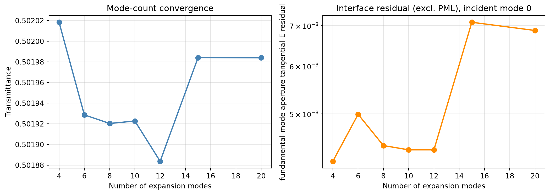
# Mode identity: effective index and TE fraction of the index-0 mode at every cell.
# Index 0 should be the quasi-TE fundamental (TE fraction ~ 1) at every cell.
modes = eme_5_data["modes"]
n_eff = modes.n_complex.real
Ey2 = (abs(modes.Ey) ** 2).sum(("x", "y", "z"))
Ez2 = (abs(modes.Ez) ** 2).sum(("x", "y", "z"))
te_fraction = (Ey2 / (Ey2 + Ez2)).real  # |Ey|² / (|Ey|² + |Ez|²)
identity = n_eff.to_dataframe(name="n_eff").join(te_fraction.to_dataframe(name="TE_fraction"))
print(identity.xs(0, level="mode_index").round(4).to_string())

# Fundamental mode (index 0), |Ey|, across the 5 cells.
fig, axes = plt.subplots(1, 5, figsize=(16, 3.2))
for cell_index, ax in enumerate(axes):
    eme_5_data.plot_field("modes", "Ey", val="abs", eme_cell_index=cell_index, mode_index=0, ax=ax)
    ax.set_title(f"cell {cell_index} — mode 0  |Ey|")
plt.tight_layout()
plt.show()
n_eff TE_fraction
f sweep_index eme_cell_index
1.934145e+14 0 0 1.6517 0.9877
1 1.6715 0.9855
2 1.6835 0.9845
3 1.6716 0.9852
4 1.6517 0.9874
Convergence Verdict
Both the transmittance and the interface residual are already flat by ~4–6 modes (residual \(\sim 5\times10^{-3}\)) and mode 0 stays the quasi-TE fundamental (TE fraction \(\approx 0.99\)) at every cell, so num_modes = 5 is sufficient and the EME plateau (~2% above FDTD) is a converged result, judged by the interface residual rather than by strict monotonicity of \(|S_{00}|^2\).


 TERMS & CONDITIONS


 How the process works:
 Try this real URL to see an example: