Note: this notebook is 90% AI-generated.
In this notebook, we will design and simulate a 2x2 Multi-Mode Interference (MMI) power splitter for photonic integrated circuits (PICs). The MMI power splitter is a fundamental component in integrated photonics, providing equal power splitting (50/50) with high efficiency.
The design follows standard Silicon-on-Insulator (SOI) platform specifications with cosine S-bends for optimal performance. We will demonstrate the complete simulation workflow including geometry setup using Photonforge and performance evaluation.
For more integrated photonic examples such as the 8-Channel mode and polarization demultiplexer, the broadband bi-level taper polarization rotator-splitter, and the broadband directional coupler, please visit our examples page.
If you are new to the finite-difference time-domain (FDTD) method, we highly recommend going through our FDTD101 tutorials.
FDTD simulations can diverge due to various reasons. If you run into any simulation divergence issues, please follow the steps outlined in our troubleshooting guide to resolve it.

Standard Python Imports
We start by importing the necessary libraries for our simulation.
# Standard python imports.
import matplotlib.pylab as plt
import numpy as np
import photonforge as pf

# Import regular tidy3d.
import tidy3d as td
import tidy3d.web as web
MMI Power Splitter Structure
The 2x2 MMI power splitter is based on a standard Silicon-on-Insulator (SOI) wafer with a device layer of 220 nm. The MMI section provides multimode interference for equal power splitting, while cosine S-bends route the input/output signals to offset positions for practical device integration.
Key Design Parameters:
- Material Platform: Silicon-on-Insulator (SOI)
- Wavelength Range: 1.5 to 1.6 μm (telecom C-band)
- Design Goal: Equal power splitting (50/50)
The MMI length is designed to achieve optimal interference patterns for equal power splitting around 1.55 micrometers, while the S-bends provide smooth transitions to offset input/output waveguides.
# MMI power splitter setup.
wavelength = 1.55  # Center simulation wavelength (um).
freq0 = td.C_0 / wavelength  # Central frequency.
# Materials.
n_si = 3.48  # Silicon refractive index.
n_sio2 = 1.44  # SiO2 refractive index.

# Material definitions.
mat_si = td.Medium(permittivity=n_si**2)  # Silicon waveguide material.
mat_sio2 = td.Medium(permittivity=n_sio2**2)  # SiO2 substrate material.
# This cell contains all the geometry, sources, monitors, and simulation creation

# MMI power splitter dimensions.
w_wg = 0.4  # Waveguide width (um).
h_si = 0.22  # Silicon layer height (um).
w_mmi = 1.0  # MMI section width (um).
l_mmi = 3.0  # MMI section length (um).
gap = 0.2  # Gap between output waveguides (um).

# Waveguide lengths.
l_input = 2.0  # Input waveguide length (um).
l_output = 3.0  # Output waveguide length (um).

# S-bend parameters.
s_bend_offset = 1.0  # Lateral offset for S-bends (um).
s_bend_length = 4.0  # Length of S-bend section (um).
Layout generation using PhotonForge
We start by creating the layout using PhotonForge’s layout capabilities. In addition to layout generation, PhotonForge also provides a complete set of tools for photonic design automation, including PDK integration, parametric components, connectivity management, and technology definitions. You can check the many applications of this powerful tool here.
We start by defining a simple pf.Rectangle structure.
Next, we use the pf.Path object, which accepts the arguments origin and width. This object can then be used to create s-bends with the built-in s_bend method, as well as straight sections with the segment method.
Finally, we use pf.boolean to combine the structures into a single polygon, and define the Tidy3D geometry as a PolySlab object.
def make_mmi_shape(
    l_mmi,
    w_mmi,
    w_wg,
    s_bend_length,
    s_bend_offset,
    center=(0, 0),
    slab_bounds=(-0.11, 0.11),
    sidewall_angle=0,
    reference_plane="top",
):

    mmi = pf.Rectangle(size=(l_mmi, w_mmi))

    x_out = l_mmi / 2
    y_out = w_mmi / 2 - w_wg / 2

    bend_out_up = pf.Path(origin=(x_out, y_out), width=w_wg)
    bend_out_up.s_bend((s_bend_length, s_bend_offset), relative=True)
    bend_out_up.segment((10, 0), relative=True)

    bend_out_down = bend_out_up.copy().mirror()
    bend_in_up = bend_out_up.copy().mirror((0, 1))
    bend_in_down = bend_out_down.copy().mirror((0, 1))

    polygons = pf.boolean(
        [
            mmi,
            bend_out_up,
            bend_out_down,
            bend_in_up,
            bend_in_down,
        ],
        [],
        "+",
    )

    assert len(polygons) == 1, "Expected a single polygon for the union."
    polygon = polygons[0]
    assert len(polygon.holes) == 0, "Expected no holes."

    polygon.translate(center)

    geometry = td.PolySlab(
        vertices=polygon.vertices,
        axis=2,
        slab_bounds=slab_bounds,
        sidewall_angle=sidewall_angle,
        reference_plane=reference_plane,
    )

    return geometry


geometry = make_mmi_shape(l_mmi, w_mmi, w_wg, s_bend_length, s_bend_offset)
mmi_structure = td.Structure(geometry=geometry, medium=mat_si)
ax = mmi_structure.plot(z=0)
Complete MMI Power Splitter Simulation Setup
Now we create the complete 2x2 MMI power splitter simulation with x-axis propagation. The simulation includes the MMI section, input/output waveguides, cosine S-bends, sources, and monitors.
# Calculate optimized simulation domain size for x-axis propagation.
x_min = -1.5 - 3.0  # -4.5 um
x_max = 5.5 + 3.0  # 8.5 um
total_length = x_max - x_min  # 13.0 um
total_width = w_mmi + 4.0  # Keep width buffer for offset waveguides
total_height = 2.0  # Sufficient for SOI structure
sim_size_optimized = (total_length, total_width, total_height)

wavelengths = np.arange(1.5, 1.61, 0.01)  # 1.5 to 1.6 μm with 10 nm steps
frequencies = td.C_0 / wavelengths

# 9. Mode source at the upper input waveguide (x-axis propagation).
source_position = (-6, 1.3, 0)
source_size = (0, 6 * w_wg, 6 * h_si)
mode_source = td.ModeSource(
    center=source_position,
    size=source_size,
    source_time=td.GaussianPulse(freq0=freq0, fwidth=freq0 / 10),
    direction="+",
    mode_spec=td.ModeSpec(num_modes=1),
    mode_index=0,
)

# 10. Mode monitors at the output waveguides (x-axis propagation).
monitor_1_position = (l_mmi / 2 + s_bend_length + 0.5, w_wg / 2 + gap / 2 + s_bend_offset, 0)
monitor_1_size = (0, 6 * w_wg, 6 * h_si)
mode_monitor_1 = td.ModeMonitor(
    center=monitor_1_position,
    size=monitor_1_size,
    freqs=frequencies,
    mode_spec=td.ModeSpec(num_modes=1),
    name="mode_output_1",
)

monitor_2_position = (l_mmi / 2 + s_bend_length + 0.5, -w_wg / 2 - gap / 2 - s_bend_offset, 0)
monitor_2_size = (0, 6 * w_wg, 6 * h_si)
mode_monitor_2 = td.ModeMonitor(
    center=monitor_2_position,
    size=monitor_2_size,
    freqs=frequencies,
    mode_spec=td.ModeSpec(num_modes=1),
    name="mode_output_2",
)

# 11. Field monitor at xy plane - record fields at specific wavelengths (x-axis propagation).
field_freqs = [td.C_0 / 1.55, td.C_0 / 1.58]  # 1.55 and 1.58 um
field_monitor = td.FieldMonitor(
    center=(0, 0, 0), size=(td.inf, td.inf, 0), freqs=field_freqs, name="field_xy"
)
# 12. Create the complete simulation.
sim_mmi = td.Simulation(
    size=sim_size_optimized,
    structures=[mmi_structure],
    sources=[mode_source],
    monitors=[mode_monitor_1, mode_monitor_2, field_monitor],
    run_time=1e-12,
    boundary_spec=td.BoundarySpec.all_sides(boundary=td.PML()),
    medium=mat_sio2,
    grid_spec=td.GridSpec(
        grid_x=td.AutoGrid(min_steps_per_wvl=20),
        grid_y=td.AutoGrid(min_steps_per_wvl=20),
        grid_z=td.AutoGrid(min_steps_per_wvl=20),
        wavelength=wavelength,
    ),
    symmetry=(0, 0, 0),
)
Simulation Visualization
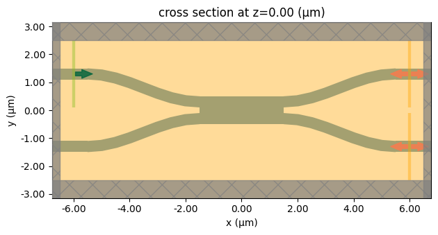
Let's visualize the complete MMI power splitter setup to verify the geometry and propagation direction.
# Simulation Setup Visualization - XY Setup Plane
fig_xy = sim_mmi.plot(z=0)  # XY cross-section at z=0 (MMI center) - shows complete setup
# 3D Visualization
fig_3d = sim_mmi.plot_3d()
Cost Estimation
Before running the simulation, let's estimate the computational cost.
# Cost Estimation
job = web.Job(simulation=sim_mmi, task_name="mmi_2x2_cost_estimation", verbose=True)
cost_info = web.estimate_cost(job.task_id)
print(f"Estimated cost: {cost_info:.4f} Flex Credits")
11:12:14 -03 Created task 'mmi_2x2_cost_estimation' with resource_id
             'fdve-1bd22af7-75e7-4c3b-8742-a73826940c73' and task_type 'FDTD'.
             View task using web UI at
             'https://tidy3d.simulation.cloud/workbench?taskId=fdve-1bd22af7-75e
             7-4c3b-8742-a73826940c73'.
Task folder: 'default'.
Output()
11:12:20 -03 Estimated FlexCredit cost: 0.077. Minimum cost depends on task
             execution details. Use 'web.real_cost(task_id)' to get the billed
             FlexCredit cost after a simulation run.
Estimated cost: 0.0772 Flex Credits
Run Simulation
Now we run the simulation to obtain the results.
# Run Simulation
sim_data = job.run(path="mmi_2x2_results.hdf5")
11:12:21 -03 Estimated FlexCredit cost: 0.077. Minimum cost depends on task
             execution details. Use 'web.real_cost(task_id)' to get the billed
             FlexCredit cost after a simulation run.
11:12:23 -03 status = queued
             To cancel the simulation, use 'web.abort(task_id)' or
             'web.delete(task_id)' or abort/delete the task in the web UI.
             Terminating the Python script will not stop the job running on the
             cloud.
Output()
11:12:43 -03 starting up solver
11:12:44 -03 running solver
Output()
11:12:56 -03 early shutoff detected at 36%, exiting.
11:12:57 -03 status = postprocess
Output()
11:13:01 -03 status = success
11:13:03 -03 View simulation result at
             'https://tidy3d.simulation.cloud/workbench?taskId=fdve-1bd22af7-75e
             7-4c3b-8742-a73826940c73'.
Output()
11:13:08 -03 Loading simulation from mmi_2x2_results.hdf5
Result Analysis
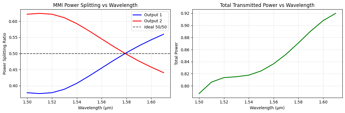
Let's analyze the simulation results to evaluate the MMI power splitter performance.
Key Performance Metrics:
-
Power Splitting Ratio: The fraction of total power that goes to each output port. For an ideal 2x2 MMI power splitter, both outputs should have a splitting ratio of 0.5 (50/50 split).
-
Total Power: The sum of power from both output ports, showing the overall transmission efficiency of the device.
# Extract mode coefficients from ModeMonitors
mode_coeff_1 = sim_data["mode_output_1"].amps.sel(mode_index=0, direction="+")
mode_coeff_2 = sim_data["mode_output_2"].amps.sel(mode_index=0, direction="+")

# Calculate power splitting
power_1 = np.abs(mode_coeff_1) ** 2
power_2 = np.abs(mode_coeff_2) ** 2
total_power = power_1 + power_2

# Calculate splitting ratio
splitting_ratio_1 = power_1 / total_power
splitting_ratio_2 = power_2 / total_power

# Ensure arrays are numpy arrays for consistent indexing
splitting_ratio_1 = np.array(splitting_ratio_1)
splitting_ratio_2 = np.array(splitting_ratio_2)
total_power = np.array(total_power)

# Create comprehensive analysis plots
fig, (ax1, ax2) = plt.subplots(1, 2, figsize=(12, 4))

# Power splitting vs wavelength
ax1.plot(wavelengths, splitting_ratio_1, "b-", label="Output 1", linewidth=2)
ax1.plot(wavelengths, splitting_ratio_2, "r-", label="Output 2", linewidth=2)
ax1.axhline(y=0.5, color="k", linestyle="--", alpha=0.7, label="Ideal 50/50")
ax1.set_xlabel("Wavelength (μm)")
ax1.set_ylabel("Power Splitting Ratio")
ax1.set_title("MMI Power Splitting vs Wavelength")
ax1.legend()
ax1.grid(True, alpha=0.3)

# Total power vs wavelength
ax2.plot(wavelengths, total_power, "g-", linewidth=2)
ax2.set_xlabel("Wavelength (μm)")
ax2.set_ylabel("Total Power")
ax2.set_title("Total Transmitted Power vs Wavelength")
ax2.grid(True, alpha=0.3)

plt.tight_layout()
plt.show()

# Print key performance metrics
print(f"Average splitting ratio 1: {splitting_ratio_1.mean():.3f}")
print(f"Average splitting ratio 2: {splitting_ratio_2.mean():.3f}")
print(f"Average total power: {total_power.mean():.3f}")
Average splitting ratio 1: 0.500
Average splitting ratio 2: 0.500
Average total power: 0.869
Power Splitting Performance Analysis:
The power splitting ratio plot reveals several important characteristics of the MMI power splitter:
-
Optimal Operating Wavelength: The device achieves perfect 50/50 splitting at approximately 1.58 μm, where both output curves intersect the ideal 50/50 line.
-
Wavelength Dependence: The splitting ratio shows significant wavelength dependence:
- At shorter wavelengths (1.50 μm): Output 2 receives ~62% of power, Output 1 receives ~37%
- At longer wavelengths (1.60 μm): Output 1 receives ~54% of power, Output 2 receives ~46%
-
Design Implications: This wavelength dependence is typical for MMI devices and can be optimized by adjusting the MMI length, width, or using apodization techniques for broader bandwidth performance.
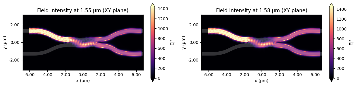
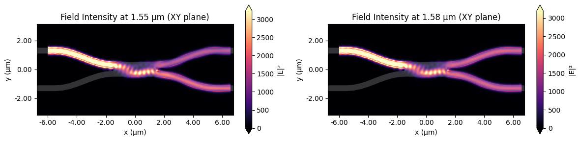
Field Intensity Analysis
Finally, let's examine the field intensity distribution at specific wavelengths in the XY plane to understand the light propagation through the MMI.
# Create a 2x1 subplot for the two wavelengths.
fig, axes = plt.subplots(1, 2, figsize=(12, 3))

# Plot field intensity at 1.55 um using Tidy3D's built-in method.
sim_data.plot_field("field_xy", "E", val="abs^2", f=td.C_0 / 1.55, ax=axes[0])
axes[0].set_title("Field Intensity at 1.55 μm (XY plane)")

# Plot field intensity at 1.58 um using Tidy3D's built-in method.
sim_data.plot_field("field_xy", "E", val="abs^2", f=td.C_0 / 1.58, ax=axes[1])
axes[1].set_title("Field Intensity at 1.58 μm (XY plane)")

plt.tight_layout()
plt.show()