





# Importing necessary libraries for simulation and visualization
import matplotlib.pyplot as plt
import numpy as np
import tidy3d as td
from tidy3d import web

# Define simulation parameters
wl = 8  # Target wavelength
cylinder_radius = 0.1  # Radii of the cylindrical antennas
fcen = td.C_0 / wl  # Central frequency
fwidth = 0.2 * fcen  # Frequency width
run_time = 2e-12  # Simulation run time
substrate_thickness = 10  # Thickness of the Si substrate
air_size = 40  # Air region to visualize the scattered fields
sx = 2 * wl  # Dimensions in the xy plane
sy = 2 * wl
sz = substrate_thickness + air_size  # Total length of the simulation
structure_z_position = -sz / 2 + substrate_thickness + cylinder_radius  # Position of the antennas
size_z_source = 2  # Size of the TFSF source
size_source = (2.5, 2.5, size_z_source)
center_source = (
    0,
    0,
    structure_z_position - cylinder_radius + size_z_source / 2,
)  # Center position of the TFSF source
TIDY3D
LEARNING CENTER
Example Library

Phase change plasmonic antennas
This notebook reproduces the phase behavior of cross-polarized scattering from gold V-shaped antennas on a silicon substrate, as demonstrated in the following paper:
Yu, N., Genevet, P., Kats, M. A., Aieta, F., Tetienne, J.-P., Capasso, F., & Gaburro, Z. (n.d.). Light Propagation with Phase Discontinuities: Generalized Laws of Reflection and Refraction. DOI: 10.1126/science.1210713.
The goal is to demonstrate the general workflow for simulating the antennas and extracting phase information from the complex monitor data. We will use two approaches:
Using a FieldMonitor with Perfectly Matched Layers (PML) to calculate the phase directly from the field values. This is an explicit approach to determine the phase of a single antenna but may require a large simulation domain. In this setup, the source is a Total-Field Scattered-Field (TFSF) source, which excites a plane wave inside its domain and only allows scattered fields to propagate outside it, allowing the phase of the scattered fields to be analyzed independently of the excitation.
Using a DiffractionMonitor with Periodic boundary conditions to extract the phase from the complex zero-order diffraction amplitude. With this method, we can assume a local periodic approximation and calculate the phase using a much smaller simulation domain. For this setup, we can use a regular PlaneWave source.
As we will see, the results from both methods match well.
A more complete example simulating the full metasurface presented in the paper can be found here.
For additional examples, check our Example Library.
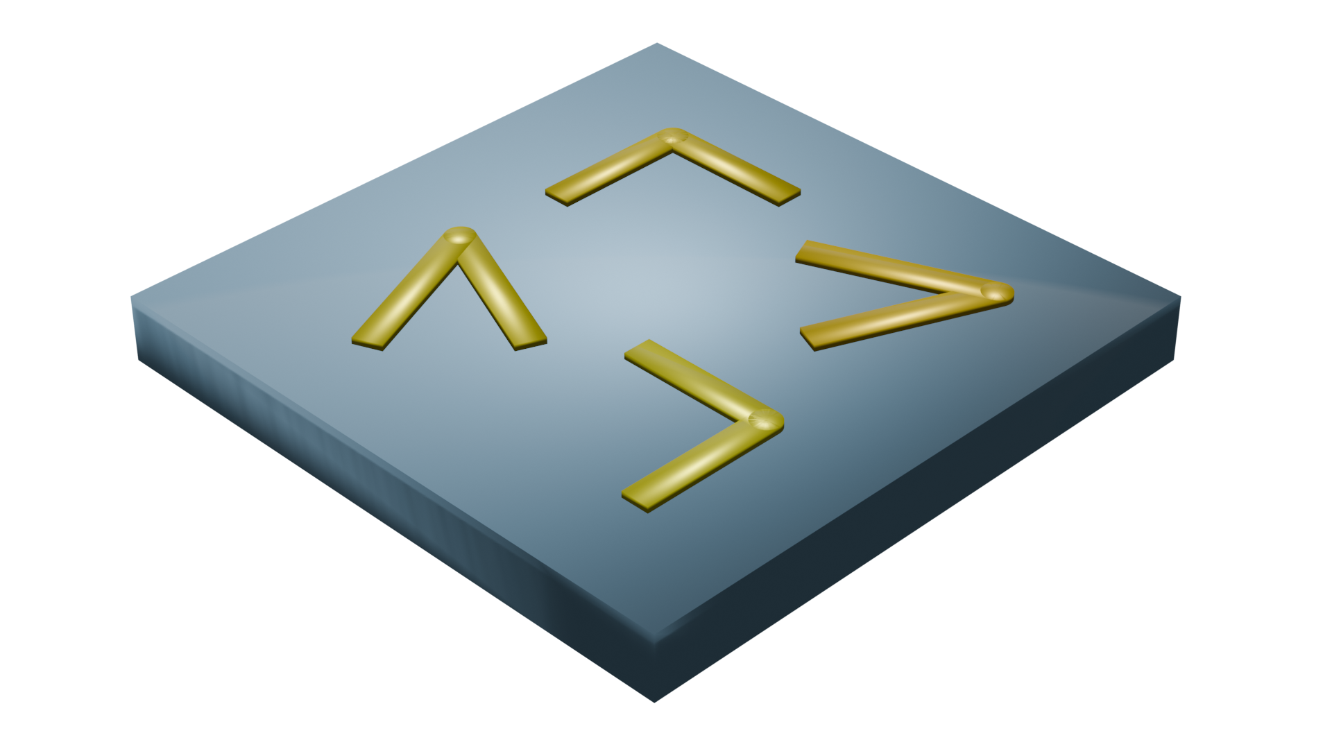
Simulation Setup
First, we define the global parameters used to create the structures.
These constants specify the wavelength, geometry, and time-domain settings shared across all antenna configurations.
Parametric V-Antenna Geometry
The helper v_antenna converts intuitive geometric inputs (arm length, opening angle, rotation) into Tidy3D primitives. Each simulation clones this geometry with different parameters to sample the phase response.
# Define the V-antenna structure
width = 0.22  # Width of the antenna arms
thickness = 0.05  # Thickness of the antenna arms


def v_antenna(center, radius, length, delta, theta):
    # Define the material properties
    medium = td.material_library["Au"]["Olmon2012crystal"]
    delta1 = (-theta + delta / 2) * np.pi / 180
    delta2 = (-theta - delta / 2) * np.pi / 180

    # Calculate offsets to centralize the antenna
    dx_to_centralize = (length / 2) * np.cos(np.deg2rad(theta))
    dy_to_centralize = (length / 2) * np.sin(np.deg2rad(theta))

    # Define the sphere at the center of the antenna
    sphere1 = td.Structure(
        geometry=td.Cylinder(radius=width / 2, center=center, axis=2, length=thickness).translated(
            -dx_to_centralize, dy_to_centralize, 0
        ),
        medium=medium,
    )

    # Define the first arm of the antenna
    dx = (length / 2) * np.cos(delta1) - dx_to_centralize
    dy = (length / 2) * np.sin(delta1) + dy_to_centralize
    c1 = (
        td.Box(size=(length, width, thickness), center=(0, 0, 0))
        .rotated(delta1, 2)
        .translated(*center)
        .translated(dx, dy, 0)
    )
    s1 = td.Structure(geometry=c1, medium=medium)

    # Define the second arm of the antenna
    dx = (length / 2) * np.cos(delta2) - dx_to_centralize
    dy = (length / 2) * np.sin(delta2) + dy_to_centralize
    c2 = (
        td.Box(center=(0, 0, 0), size=(length, width, thickness))
        .rotated(delta2, 2)
        .translated(*center)
        .translated(dx, dy, 0)
    )
    s2 = td.Structure(geometry=c2, medium=medium)

    return [s1, s2, sphere1]  # Return the antenna components


# Dictionary containing the length and angle parameters of the 8 antennas
dic_numerator = {
    0: (180, 45, 0.75),
    1: (45, -45, 1.35),
    2: (-90, -45, 1.12),
    3: (-90 - 45, -45, 0.95),
    4: (180, -45, 0.75),
    5: (45, 45, 1.35),
    6: (90, 45, 1.12),
    7: (90 + 45, 45, 0.95),
}
Mesh Override and Source Placement
Since the structures are much smaller than the target wavelength, it is convenient to create a mesh override region around the metasurface to properly resolve the structures, while using a coarser mesh in the free-space propagation region.
Because the TFSF source performs best in a uniform mesh, the size and position of the override region are set equal to those of the source.
# Define the mesh override region
mesh_override = td.MeshOverrideStructure(
    geometry=td.Box(center=center_source, size=size_source), dl=(0.02, 0.02, 0.02)
)

# Redefine positions for the new geometry
structure_z_position = -sz / 2 + substrate_thickness + thickness / 2
size_z_source = 2
size_source = (2.5, 2.5, size_z_source)
center_source = (0, 0, structure_z_position - thickness / 2 + size_z_source / 2)

# Define the TFSF source
source_time = td.GaussianPulse(freq0=fcen, fwidth=fwidth)
source = td.TFSF(
    center=center_source,
    size=size_source,
    direction="+",
    injection_axis=2,
    pol_angle=0,
    source_time=source_time,
)
# Adding monitors to keep track of the field profile at the target frequency
field_mon_y = td.FieldMonitor(
center=(0, 0, 0), size=(td.inf, 0, td.inf), freqs=[fcen], name="field_mon_y"
)
field_mon_x = td.FieldMonitor(
center=(0, 0, 0), size=(0, td.inf, td.inf), freqs=[fcen], name="field_mon_x"
)Simulation using FieldMonitor and PML
Now, we can create the simulation object, defining the boundaries as PMLs.
A silicon substrate and absorbing boundaries define the background structure. We reuse this template with different antenna geometries to form the full batch submission.
# Defining the structure modeling the substrate
substrate = td.Structure(
    geometry=td.Box(center=(0, 0, -sz / 2), size=(2 * sx, 2 * sy, 2 * substrate_thickness)),
    medium=td.Medium(permittivity=3.47**2),
)


# Defining the base simulation
sim = td.Simulation(
    size=(sx, sy, sz),
    grid_spec=td.GridSpec.auto(override_structures=[mesh_override]),
    structures=[],
    sources=[source],
    monitors=[field_mon_y, field_mon_x],
    run_time=run_time,
    boundary_spec=td.BoundarySpec(x=td.Boundary.pml(), y=td.Boundary.pml(), z=td.Boundary.pml()),
)
Next, we create a dictionary containing one simulation for each antenna.
simulations = {}
fig, axes = plt.subplots(2, 4, figsize=(12, 10), constrained_layout=True)

for key, ax in zip(range(8), axes.flatten()):
    delta, theta, length = dic_numerator[key]
    antenna = v_antenna(
        center=(0, 0, structure_z_position),
        radius=cylinder_radius,
        length=length,
        delta=delta,
        theta=theta,
    )

    name = f"ScatteringCylinder_{key}"
    simulations[name] = sim.updated_copy(structures=antenna + [substrate])

    # Plot the simulation with monitor_alpha=0 and source_alpha=0
    simulations[name].plot(z=structure_z_position, ax=ax, monitor_alpha=0, source_alpha=0)

    # Calculate the phase applied by the antenna (example calculation)
    applied_phase = key * (np.pi / 4)  # Assuming phase steps of π/4
    applied_phase_deg = np.degrees(applied_phase)  # Convert to degrees

    # Set the title with the phase
    ax.set_title(f"Phase: {applied_phase_deg:.1f}°", fontsize=24)

    # Remove axis labels and ticks
    ax.axis("off")
    ax.set_xlim(-1, 1)
    ax.set_ylim(-1, 1)

# Show the figure
plt.show()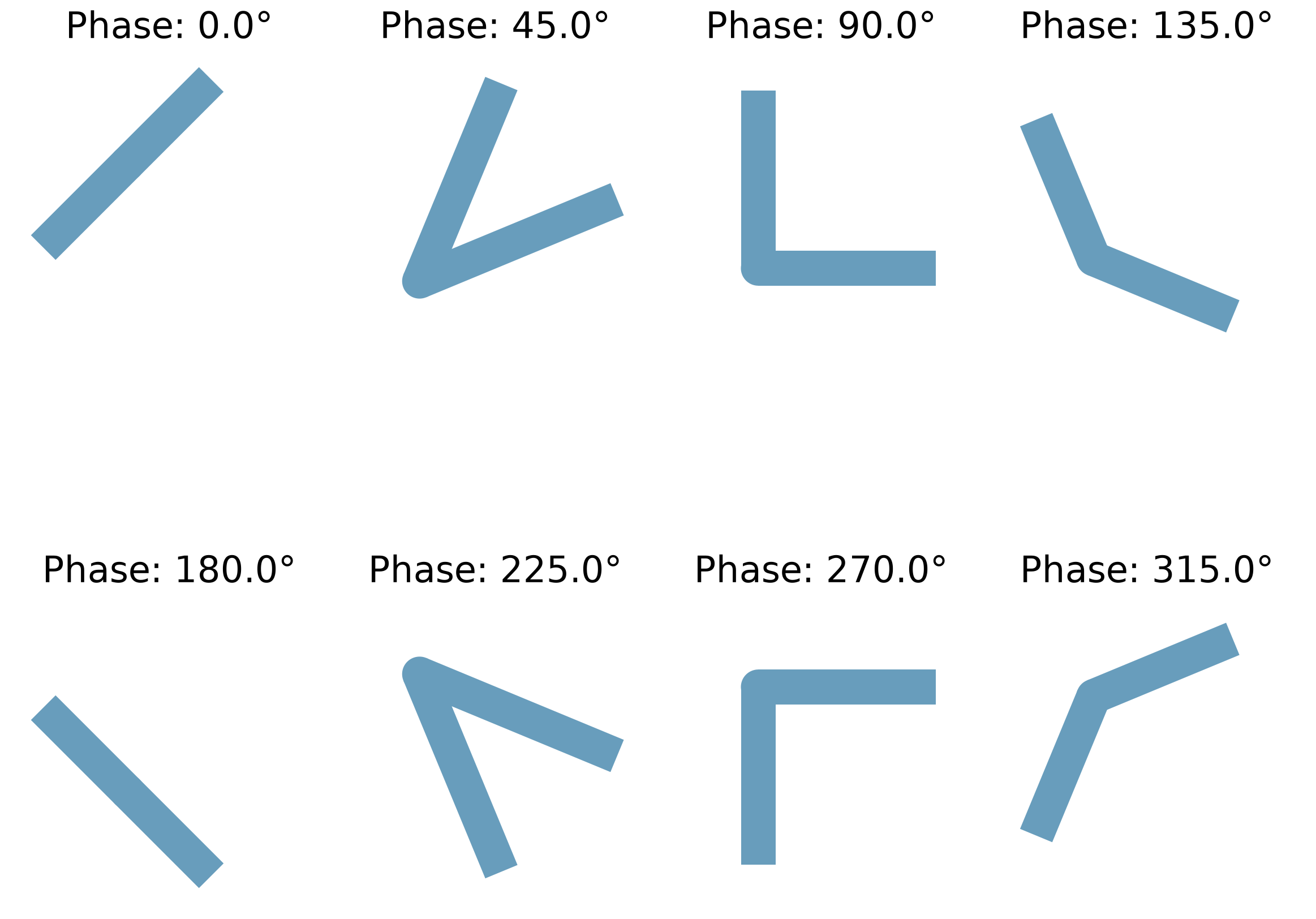
Before running the simulation, we can visualize the setup to ensure everything is correctly placed.
simulations["ScatteringCylinder_0"].plot_3d()Running the Batch Simulation
Now we create and run a Batch simulation, which executes the eight simulations in parallel.
# Creating the batch object
batch = web.Batch(simulations=simulations, verbose=True)

# Running the batch
results = batch.run(path_dir="dataScatteringCylinders")
10:32:43 UTC Started working on Batch containing 8 tasks.
10:32:49 UTC Maximum FlexCredit cost: 1.575 for the whole batch.
             Use 'Batch.real_cost()' to get the billed FlexCredit cost after
             completion.
10:36:30 UTC Batch complete.
Visualizing Scattered Amplitude and Phase
First, we visualize the Ey field component and its phase.
Since the fields are complex values, the phase can be easily calculated using the np.angle function.
# Plotting the scattered fields and phases
N = len(simulations)
fig, axes = plt.subplots(2, int(N / 2), figsize=(5 * int(N / 2), 12), constrained_layout=True)
keys = list(simulations.keys())
for col, i in enumerate(range(0, N, 2)):
    key = keys[i]
    result = results[key]
    field = result["field_mon_y"].Ey.squeeze()
    x = result["field_mon_y"].Ey.x.squeeze()
    z = result["field_mon_y"].Ey.z.squeeze()

    amplitude = field.real.T
    phase = np.angle(field).T

    axes[0, col].pcolormesh(x, z, amplitude, vmin=-0.5, vmax=0.5, cmap="RdBu_r")
    axes[0, col].set_title(f"Antenna {key}Re(Ey)", fontsize=14)
    axes[0, col].axis("off")

    axes[1, col].pcolormesh(x, z, phase, vmin=-np.pi, vmax=np.pi, cmap="twilight")
    axes[1, col].set_title("Phase (rad)", fontsize=12)
    axes[1, col].axis("off")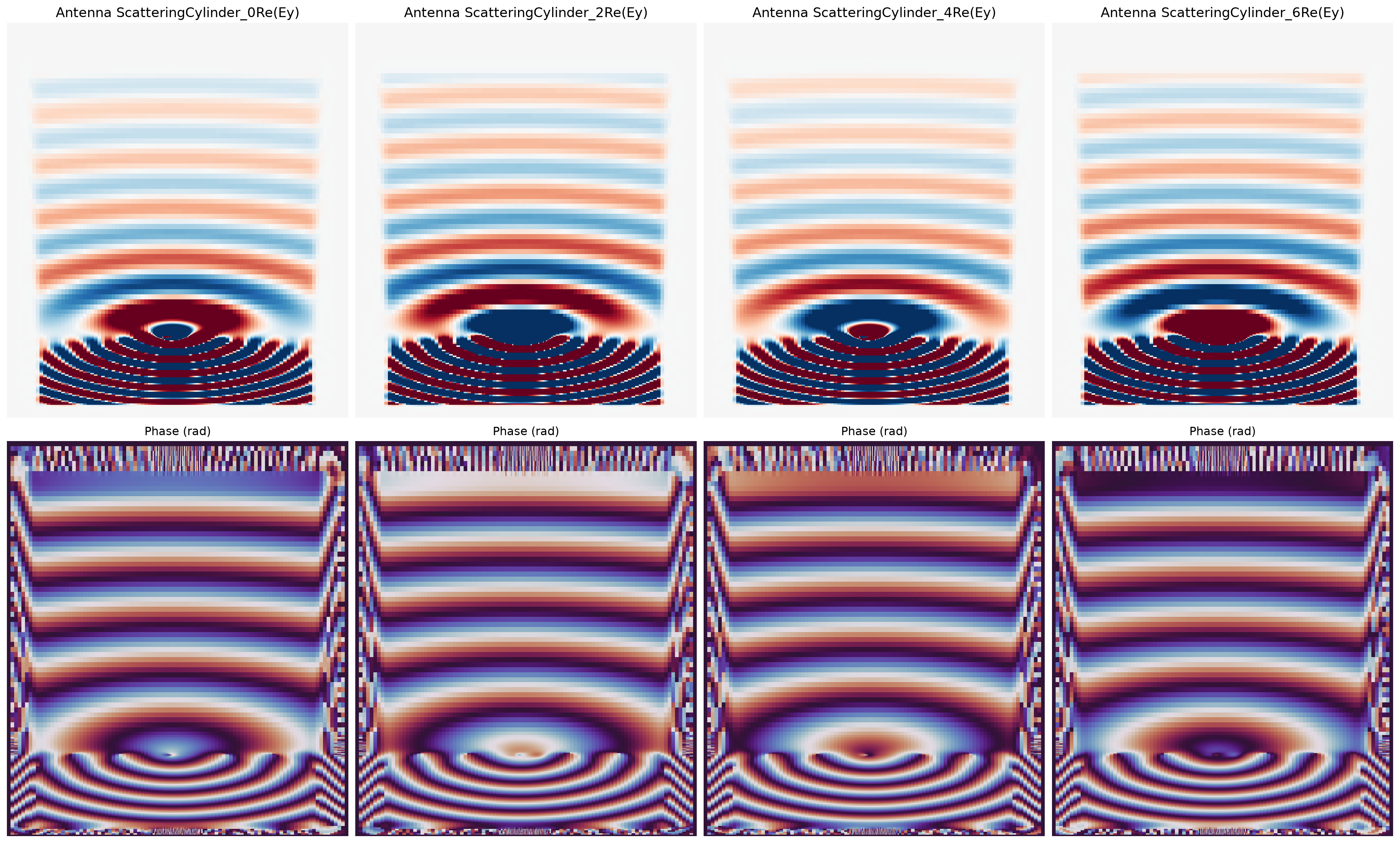
As we can see, the phase of the transmitted fields increases across different antennas.
Extracting On-Axis Phase Delays
We probe the center of the field_mon_y plane, compute the complex phase, and reference everything to antenna 0.
It can be observed that the antennas provide a continuous phase variation over 360 degrees.
# Collect phase at monitor intersection for each antenna
phases = []
for name in simulations:
    monitor = results[name]["field_mon_y"]
    value = monitor.Ey.sel(z=20, method="nearest").squeeze()
    phases.append(np.angle(np.mean(value.data)))

phases = np.array(phases)
# Reference all phases to antenna 0
phase_deg = -np.degrees(np.unwrap(phases - phases[0]))
# Bar chart summarizing relative phase at z = 0
fig, ax = plt.subplots(figsize=(6, 4))
indices = np.arange(len(phase_deg))
ax.bar(indices, phase_deg)
ax.set_xticks(indices)
ax.set_xticklabels(list(simulations.keys()), rotation=45, ha="right")
ax.set_ylabel("Phase shift (deg) relative to antenna 0")
ax.set_title("Cross-polarized phase at x = 0, z = 0")
ax.axhline(0, color="k", linewidth=0.8)
ax.grid(True, axis="y", alpha=0.3)
fig.tight_layout()
# Tabulate numeric values for quick inspection
print("Phase shift summary (deg):")
for name, value in zip(simulations.keys(), phase_deg):
print(f" {name}: {value:.2f}")Phase shift summary (deg):
ScatteringCylinder_0: -0.00
ScatteringCylinder_1: 38.02
ScatteringCylinder_2: 107.02
ScatteringCylinder_3: 162.12
ScatteringCylinder_4: 180.00
ScatteringCylinder_5: 218.02
ScatteringCylinder_6: 287.02
ScatteringCylinder_7: 342.12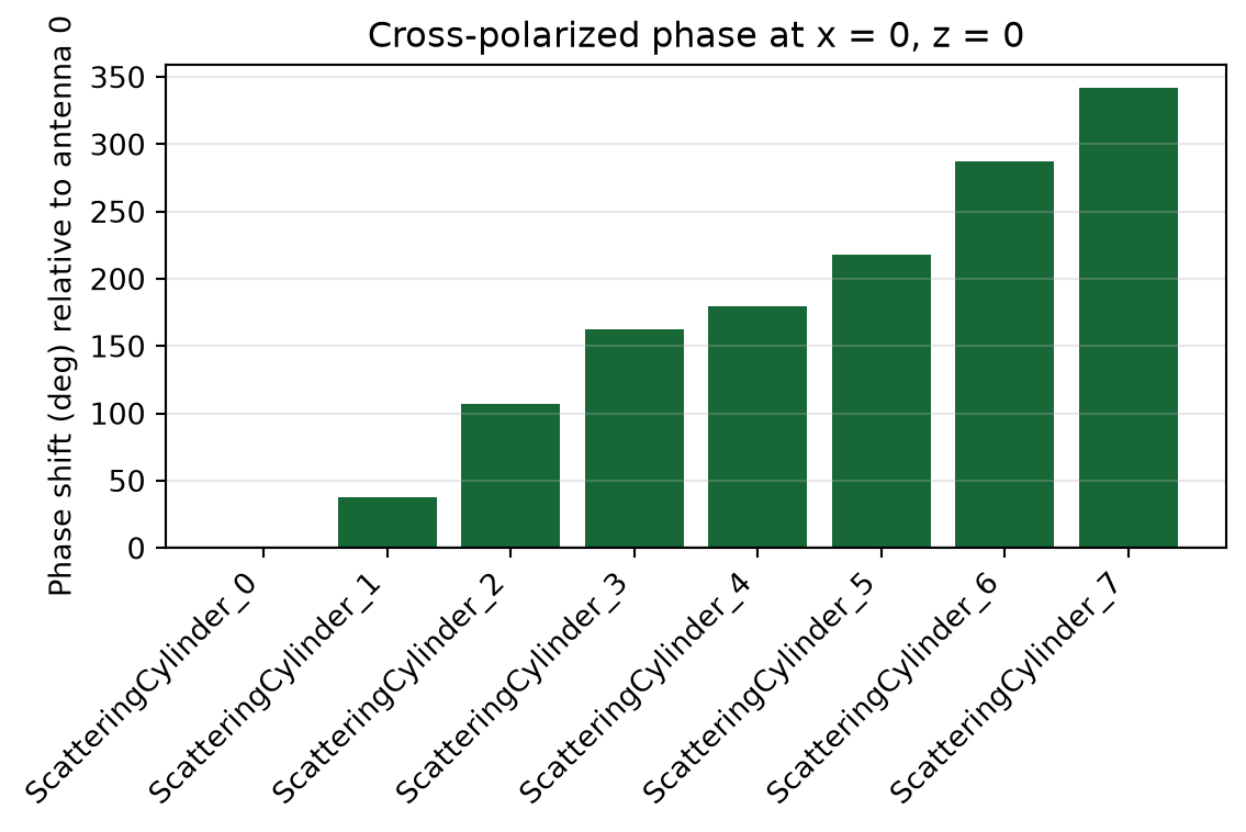
Phase calculation using a DiffractionMonitor and periodic boundary conditions
Now, we can adapt the simulations from the previous section to use periodic boundaries and replace the FieldMonitor with a DiffractionMonitor. We will also replace the TFSF source with a PlaneWave source.
With this approach, we can also reduce the simulation size in the z-direction.
# Define boundary conditions: periodic in x and y, PML absorbing boundaries in z
boundary_spec = td.BoundarySpec(
    x=td.Boundary.periodic(), y=td.Boundary.periodic(), z=td.Boundary.pml()
)

# Set simulation domain center and size for periodic setup
sim_periodic_center = (0, 0, structure_z_position)
sim_periodic_size = (sx, sy, 2 * wl)

# Create a diffraction monitor above the structure to capture transmitted/reflected fields
diffraction_monitor = td.DiffractionMonitor(
    center=(0, 0, structure_z_position + wl - 1),
    size=(td.inf, td.inf, 0),
    freqs=[fcen],
    name="diffraction_monitor",
)

# Define a plane wave source below the structure
pw_source = td.PlaneWave(
    center=(0, 0, structure_z_position - wl + 1),
    size=(td.inf, td.inf, 0),
    source_time=td.GaussianPulse(freq0=fcen, fwidth=fwidth),
    name="pw_source",
    direction="+",
)

# Creating the simulation dictionary for the Batch
sims_periodic = {
    i: simulations[i].updated_copy(
        boundary_spec=boundary_spec,
        monitors=[diffraction_monitor],
        sources=[pw_source],
        size=sim_periodic_size,
        center=sim_periodic_center,
    )
    for i in simulations.keys()
}
# Visualizing the setup
sims_periodic["ScatteringCylinder_0"].plot_3d()# Running the Batch
batch_periodic = web.Batch(simulations=sims_periodic, verbose=True)
results_periodic = batch_periodic.run(path_dir="dataScatteringCylindersPeriodic")10:36:40 UTC Started working on Batch containing 8 tasks.
10:36:46 UTC Maximum FlexCredit cost: 0.969 for the whole batch.
             Use 'Batch.real_cost()' to get the billed FlexCredit cost after
             completion.
10:37:24 UTC Batch complete.
Now, we can analyze the amplitude of the first diffraction order of the cross-polarized component and again use np.angle to extract the phase.
As we can see, the results match very well with those from the previous setup.
phase_s = []
phase_p = []

for k in results_periodic.keys():
    sim_data_periodic = results_periodic[k]
    diffraction_data = sim_data_periodic["diffraction_monitor"]
    phase_s.append(np.angle(diffraction_data.amps.sel(orders_x=0, orders_y=0, polarization="s"))[0])
phase_s = np.array(phase_s)
# Reference all phases to antenna 0
phase_deg_periodic = -np.degrees(np.unwrap(phase_s - phase_s[0]))
# Bar chart summarizing relative phase at z = 0
fig_periodic, ax_periodic = plt.subplots(figsize=(6, 4))
indices_periodic = np.arange(len(phase_deg_periodic))
ax_periodic.bar(indices_periodic, phase_deg_periodic)
ax_periodic.set_xticks(indices_periodic)
ax_periodic.set_xticklabels(list(sims_periodic.keys()), rotation=45, ha="right")
ax_periodic.set_ylabel("Phase shift (deg) relative to antenna 0")
ax_periodic.set_title("Cross-polarized phase at x = 0, z = 0 (periodic)")
ax_periodic.axhline(0, color="k", linewidth=0.8)
ax_periodic.grid(True, axis="y", alpha=0.3)
fig_periodic.tight_layout()
# Tabulate numeric values for quick inspection
print("Phase shift summary (deg) - periodic:")
for name, value in zip(sims_periodic.keys(), phase_deg_periodic):
print(f" {name}: {value:.2f}")Phase shift summary (deg) - periodic:
ScatteringCylinder_0: -0.00
ScatteringCylinder_1: 38.07
ScatteringCylinder_2: 107.33
ScatteringCylinder_3: 162.14
ScatteringCylinder_4: 180.00
ScatteringCylinder_5: 218.07
ScatteringCylinder_6: 287.33
ScatteringCylinder_7: 342.14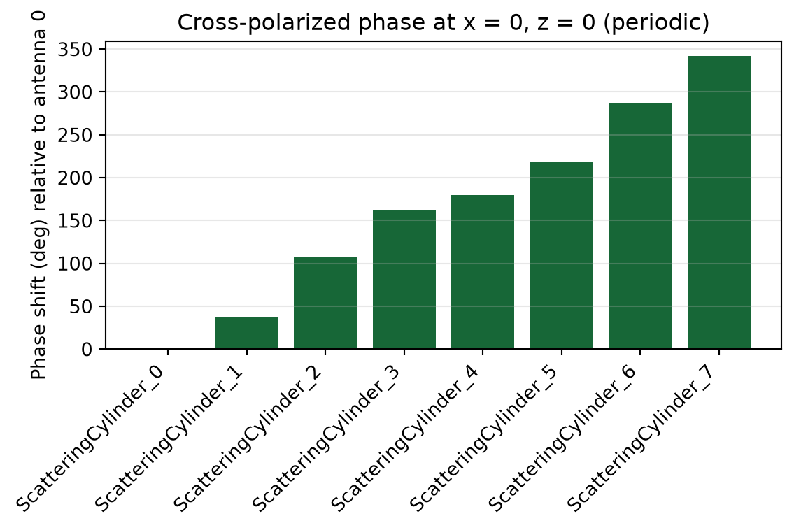
No matching results found.


 TERMS & CONDITIONS


 How the process works:
 Try this real URL to see an example: