PHOTONFORGE
LEARNING CENTER

Frequently Asked Questions

How to estimate the cost of an S matrix computation?

When using a Tidy3DModel, the cost can be estimated with the Tidy3DModel.estimate_cost() function. An example can be found in the Tidy3D Model guide.

How to change the layers of a component?

The function Component.remap_layers() can be used to efficiently remap the existing layers into new ones.

Can I use paths to create corrugated waveguides?

Yes, by parametrizing the width (and optionally the offset) of the path. The parametrization uses an Expression to define the value and the derivative of the value for the width (or offset) along the path. Here's an example:

w0 = 0.5
dw = 0.1
scale = 50 * np.pi
width = pf.Expression(
    "u",
    [
        ("w", f"{w0} + {dw} * sin({scale} * u)"),
        ("dw_du", f"{dw * scale} * cos({scale} * u)"),
    ],
)

# Ring with both sides corrugated from the width expression
both_sides = pf.Path((0, 0), width(0)[0])
both_sides.arc(-90, 270, radius=5, width=width)

offset = pf.Expression(
    "u",
    [
        ("q", f"{-0.5 * dw} * sin({scale} * u)"),
        ("dq_du", f"{-0.5 * dw * scale} * cos({scale} * u)"),
    ],
)

# Single side corrugation by adjusting the central offset to compensate
# half of the width corrugation
one_side = pf.Path((15, 0), width(0)[0], offset(0)[0])
one_side.arc(-90, 270, radius=5, width=width, offset=offset)

How do I specify the number of vertices when a circle or a path is converted to a polygon?

You can set min_evals for Circle and Path objects to define the minimum number of points used when converting arcs in these shapes to polygonal lines. The actual number of points will be increased if necessary to ensure that config.tolerance is maintained.

How do I apply changes to a simulation object in a mode solver simulation?

You can use the updated_copy() method to apply changes. This function creates a new object with the specified properties updated, without modifying the original object.

For example, the following line applies y-symmetry to a mode solver simulation:

mode_solver.simulation.updated_copy(symmetry=(0, -1, 0))

This same approach can be used to update other simulation object properties — such as grid spacing, boundary conditions, or source definitions — by calling updated_copy() on the relevant part of the simulation and passing the desired new values as arguments.

How can I extract simulation data, such as field data, from Tidy3D?

You can extract simulation data from Tidy3D by accessing the Tidy3DModel.batch_data_for() method on your active model. This allows you to retrieve data associated with a specific simulation object. Once you have the simulation data, you can then plot a specific field component, such as "Ey", using the Tidy3DFieldData.plot_field() method, as demonstrated in the example below:

sim_data = c.active_model.batch_data_for(c)
_ = sim_data["P0@0"].plot_field("field", "Ey", robust=False)

In the above example, c is the component and "field" is the name of a field monitor defined in the component's model.

How can I simulate the S-matrix exclusively for a specific port?

To simulate the S-matrix exclusively for a specific port, you can pass the model_kwargs argument to the Component.s_matrix() call.

For example, to simulate the S-matrix using only port "P0" as the input:

s_matrix = c.s_matrix(freqs, model_kwargs={"inputs": ["P0"]})

How do I update a specific reference within a hierarchical component, such as its model?

You can update specific references within a hierarchical component by using a nested dictionary. The outer dictionary's keys define the reference path starting from the top-level component, using a tuple of the form (reference name, reference index, ...).

The corresponding value is another dictionary that can include keys like "model_updates" (or other valid update types), which then maps variable names to their new values.

Here's an illustrative example from the Switch Array notebook:

updates = {
    ("Unit Cell", 14, "Tunable MZI", 0, "Phase Shifter", 0): {
        "model_updates": {"n_complex": index(v_bar)}
    }
}

s_matrix = switch_array.s_matrix(
    pf.C_0 / wavelengths, model_kwargs={"updates": updates}
)

This mechanism allows fine-grained control over deeply nested components without modifying the original design.

How do I define port symmetries?

To define port symmetries, you should specify different port orderings that leave the S-matrix of the device unchanged. This is common for symmetric components like directional couplers.

Port symmetries are defined by listing alternative sequences of the output ports that correspond to equivalent physical configurations. Each tuple represents a reordering of the ports, where the ith element in the tuple is the port that replaces port Pi in the new configuration.

For example, consider a directional coupler with four ports labeled P0, P1, P2, and P3 in a rectangular layout:

• Swapping P0 with P1 and P2 with P3 corresponds to a reflection across the x-axis.
• Swapping P0 with P2 and P1 with P3 corresponds to a reflection across the y-axis.
• Swapping P0 with P3 and P1 with P2 corresponds to a 180° rotation (inversion symmetry).

These symmetries can be encoded as:

port_symmetries = [
    ("P1", "P0", "P3", "P2"),  # x-axis reflection
    ("P2", "P3", "P0", "P1"),  # y-axis reflection
    ("P3", "P2", "P1", "P0"),  # inversion symmetry
]

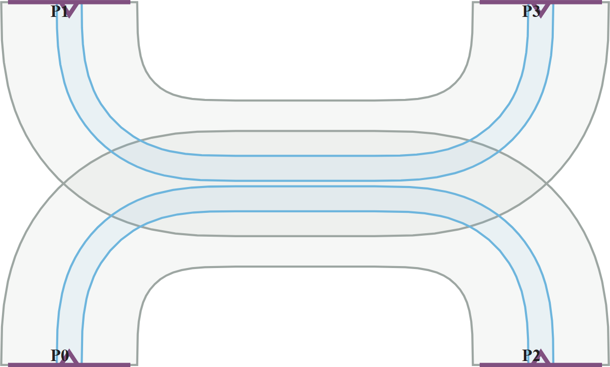
After defining symmetries, it is strongly recommended to validate them using the Tidy3DModel.test_port_symmetries() function. For faster validation, use a coarse grid and a single frequency point:

assert dc.active_model.test_port_symmetries(
    dc, frequencies=[pf.C_0 / 1.55], grid_spec=8
)

Is the order of ExtrusionSpec objects in a list important?

Yes, the order of ExtrusionSpec objects within a list is crucial, as it determines the sequence in which the extrusion operations are applied. This is particularly important for hierarchical extrusions or when one extrusion depends on the geometry created by a previous one.

In most cases, the order should follow the physical sequence of fabrication steps, ensuring that layers are built up in the correct order.

How can I modify a technology?

If the technology is parametric, you can update its parameters — such as layer thicknesses or medium definitions — either when first instantiating it or later by using the Technology.update() method.

You can also modify the structure of the technology by:

• Adding or removing layers using Technology.add_layer() and Technology.remove_layer()
• Adding or removing ports using Technology.add_port() and Technology.remove_port()
• Defining or deleting connections between layers using Technology.add_connection() and Technology.remove_connection()
• Managing extrusion specifications using Technology.insert_extrusion_spec() and Technology.pop_extrusion_spec()

These capabilities give you full control over the technology stack to match your fabrication requirements.