Author: Donghee Lee, University of Seoul
This notebook designs and analyzes a compact 1×2 multimode-interference (MMI) splitter using Tidy3D FDTD.
The device is framed as a primitive for photonic integrated circuits (PICs) and photonic neural networks: a 50:50 splitter is a basic building block for interferometric meshes, optical matrix multiplication hardware, coherent photonic circuits, and programmable photonic processors.
What This Notebook Demonstrates
- A clean 2D effective-index FDTD model of a PIC component.
- Mode source excitation of a single input waveguide.
- Modal power extraction at two output waveguides via ModeMonitor.
- A compact parameter sweep over MMI length.
- Robust cloud execution helpers for temporary HTTP 502/503/504 errors.
- Field visualization for the best design.
- A short convergence check over grid resolution.
Setup
If this is your first time using Tidy3D, please follow the Start Here guide to install the package and configure your API key.
import re
from pathlib import Path

import numpy as np
import pandas as pd
import matplotlib.pyplot as plt
from IPython.display import display, Image

import tidy3d as td
import tidy3d.web as web

# Keep repeated non-fatal geometry warnings from cluttering the submission notebook.
# Remove this line while debugging geometry if you want to see all Tidy3D warnings.
td.config.logging_level = "ERROR"

print("Tidy3D version:", td.__version__)
print("NumPy version:", np.__version__)

DATA_DIR = Path("data_mmi_splitter")
DATA_DIR.mkdir(exist_ok=True)

SWEEP_CSV = DATA_DIR / "mmi_length_sweep_results.csv"
CONV_CSV = DATA_DIR / "mmi_convergence_check.csv"
FIELD_PNG = DATA_DIR / "best_mmi_field.png"
FIELD_HDF5 = DATA_DIR / "best_mmi_field.hdf5"
Tidy3D version: 2.10.2
NumPy version: 2.4.4
1. Device Concept
A 1×2 MMI splitter uses self-imaging in a wider multimode region. Light injected from the input waveguide excites several lateral modes inside the MMI. At an appropriate propagation length, the interference pattern forms two nearly equal images at the output waveguide positions.
Here we use a 2D effective-index approximation. This is not a final foundry-ready 3D device; it is a compact FDTD example for studying the device physics and workflow.
# Units: Tidy3D uses micrometers for length.
um = 1.0

# Wavelength and frequency setup.
lambda0 = 1.55 * um
freq0 = td.C_0 / lambda0
fwidth = 0.12 * freq0
freqs = np.array([freq0])

# 2D effective-index model.
# These are typical effective-index-like values, not a specific foundry stack.
n_core = 2.80
n_clad = 1.44

core = td.Medium(permittivity=n_core**2)
clad = td.Medium(permittivity=n_clad**2)

# Waveguide and MMI geometry.
wg_width = 0.45 * um
mmi_width = 3.20 * um
output_sep = 1.05 * um

input_len = 2.0 * um
output_len = 2.0 * um

# Simulation domain padding.
pad_x = 1.0 * um
pad_y = 1.2 * um

# Temporal and numerical settings.
min_steps_per_wvl_default = 30
run_time = 1.8e-12

# Compact MMI length sweep.
mmi_lengths = np.linspace(3.8, 6.2, 9) * um

print("Number of MMI lengths:", len(mmi_lengths))
print("MMI length sweep [um]:", np.round(mmi_lengths, 3))
Number of MMI lengths: 9
MMI length sweep [um]: [3.8 4.1 4.4 4.7 5.  5.3 5.6 5.9 6.2]
2. Simulation Builder
The function below builds a single 2D FDTD Simulation for a selected MMI length. ModeMonitor objects are placed at the output ports to estimate the guided power in the fundamental mode of each output waveguide.
def make_mmi_sim(
    mmi_length,
    min_steps_per_wvl=min_steps_per_wvl_default,
    include_field_monitor=False,
):
    """Create a 2D effective-index Tidy3D simulation for a 1x2 MMI splitter."""

    x_total = input_len + mmi_length + output_len + 2 * pad_x
    y_total = mmi_width + 2 * pad_y

    x_mmi_start = -mmi_length / 2
    x_mmi_end = +mmi_length / 2

    x_source = -x_total / 2 + 0.55 * pad_x
    x_monitor = x_total / 2 - 0.55 * pad_x

    # Extend the input/output waveguides one wavelength past the simulation
    # boundary so the structures pass entirely through the PML layers and
    # the absorbed wave is the guided mode (no waveguide-tip reflection).
    x_input_left = -x_total / 2 - lambda0
    x_input_right = x_mmi_start
    x_input_center = (x_input_left + x_input_right) / 2
    input_section_length = x_input_right - x_input_left

    x_output_left = x_mmi_end
    x_output_right = x_total / 2 + lambda0
    x_output_center = (x_output_left + x_output_right) / 2
    output_section_length = x_output_right - x_output_left

    y_top = +output_sep / 2
    y_bottom = -output_sep / 2

    structures = [
        td.Structure(
            geometry=td.Box(
                center=(x_input_center, 0, 0),
                size=(input_section_length, wg_width, td.inf),
            ),
            medium=core,
            name="input_waveguide",
        ),
        td.Structure(
            geometry=td.Box(
                center=(0, 0, 0),
                size=(mmi_length, mmi_width, td.inf),
            ),
            medium=core,
            name="mmi_region",
        ),
        td.Structure(
            geometry=td.Box(
                center=(x_output_center, y_top, 0),
                size=(output_section_length, wg_width, td.inf),
            ),
            medium=core,
            name="top_output_waveguide",
        ),
        td.Structure(
            geometry=td.Box(
                center=(x_output_center, y_bottom, 0),
                size=(output_section_length, wg_width, td.inf),
            ),
            medium=core,
            name="bottom_output_waveguide",
        ),
    ]

    pulse = td.GaussianPulse(freq0=freq0, fwidth=fwidth)
    mode_spec = td.ModeSpec(num_modes=1, target_neff=n_core)

    source = td.ModeSource(
        center=(x_source, 0, 0),
        size=(0, 2.2 * wg_width, td.inf),
        source_time=pulse,
        direction="+",
        mode_spec=mode_spec,
        mode_index=0,
        name="input_mode",
    )

    monitors = [
        td.ModeMonitor(
            center=(x_monitor, y_top, 0),
            size=(0, 2.4 * wg_width, td.inf),
            freqs=freqs,
            mode_spec=mode_spec,
            name="top_mode",
        ),
        td.ModeMonitor(
            center=(x_monitor, y_bottom, 0),
            size=(0, 2.4 * wg_width, td.inf),
            freqs=freqs,
            mode_spec=mode_spec,
            name="bottom_mode",
        ),
    ]

    if include_field_monitor:
        monitors.append(
            td.FieldMonitor(
                center=(0, 0, 0),
                size=(td.inf, td.inf, 0),
                freqs=freqs,
                fields=["Ex", "Ey", "Ez"],
                name="field_xy",
            )
        )

    return td.Simulation(
        size=(x_total, y_total, 0),
        medium=clad,
        structures=structures,
        sources=[source],
        monitors=monitors,
        run_time=run_time,
        boundary_spec=td.BoundarySpec.all_sides(boundary=td.PML()),
        grid_spec=td.GridSpec.auto(min_steps_per_wvl=min_steps_per_wvl),
    )
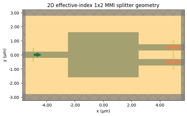
3. Geometry Preview
The plot below checks the 2D layout before submitting any jobs.
preview_sim = make_mmi_sim(
    mmi_lengths[len(mmi_lengths) // 2], include_field_monitor=True
)

fig, ax = plt.subplots(figsize=(9, 4))
preview_sim.plot(z=0, ax=ax)
ax.set_title("2D effective-index 1x2 MMI splitter geometry")
plt.show()
4. Post-processing Helpers
Helpers that turn a completed batch into a tidy result table: extract the forward fundamental-mode power at each output port and score the splitter.
def length_from_task_name(task_name):
    """Extract MMI length from a task name like 'L_3.800um'."""

    match = re.search(r"L_([0-9.]+)um", str(task_name))
    if match is None:
        raise ValueError(f"Could not extract MMI length from task name: {task_name}")
    return float(match.group(1))


def extract_forward_mode_power(sim_data, monitor_name, mode_index=0):
    """Extract forward fundamental-mode power |a+|^2 from a Tidy3D ModeMonitor."""

    amps = sim_data[monitor_name].amps
    amp = amps.sel(direction="+", mode_index=mode_index).values
    amp = np.asarray(amp).squeeze()
    return float(np.abs(amp) ** 2)


def score_splitter(p_top, p_bottom):
    """Return useful MMI splitter performance metrics."""

    p_total = p_top + p_bottom
    imbalance = abs(p_top - p_bottom) / max(p_total, 1e-30)
    split_score = p_total * (1 - imbalance)
    insertion_loss_db = -10 * np.log10(max(p_total, 1e-30))

    return {
        "P_top": p_top,
        "P_bottom": p_bottom,
        "P_total": p_total,
        "imbalance": imbalance,
        "split_score": split_score,
        "insertion_loss_dB": insertion_loss_db,
    }


def summarize_mmi_batch(batch_results, output_csv):
    """Convert a completed MMI BatchData object into a clean result table."""

    rows = []
    for task_name in batch_results.keys():
        sim_data = batch_results[task_name]
        length_um = length_from_task_name(task_name)
        p_top = extract_forward_mode_power(sim_data, "top_mode")
        p_bottom = extract_forward_mode_power(sim_data, "bottom_mode")
        metrics = score_splitter(p_top, p_bottom)

        rows.append(
            {
                "task": task_name,
                "mmi_length_um": length_um,
                **metrics,
            }
        )

    df = pd.DataFrame(rows)
    df = df.sort_values("mmi_length_um").reset_index(drop=True)
    df.to_csv(output_csv, index=False)
    return df
5. MMI Length Sweep
This cell submits a small batch of FDTD jobs unless a cached CSV already exists.
if SWEEP_CSV.exists():
    print(f"Loading cached sweep results from: {SWEEP_CSV}")
    sweep_df = pd.read_csv(SWEEP_CSV)
else:
    sweep_sims = {
        f"L_{float(L):.3f}um": make_mmi_sim(L, include_field_monitor=False)
        for L in mmi_lengths
    }

    sweep_batch = web.Batch(simulations=sweep_sims, verbose=True)
    sweep_batch_results = sweep_batch.run(path_dir=str(DATA_DIR / "sweep"))

    sweep_df = summarize_mmi_batch(
        batch_results=sweep_batch_results,
        output_csv=SWEEP_CSV,
    )
    print(f"Saved results to: {SWEEP_CSV}")

display(sweep_df)

best_row = sweep_df.sort_values("split_score", ascending=False).iloc[0]
best_length = float(best_row["mmi_length_um"]) * um

print("\nBest MMI length:")
display(best_row)
print(f"Best length = {best_length:.3f} um")
Output()
14:42:00 -03 Started working on Batch containing 9 tasks.
14:42:14 -03 Maximum FlexCredit cost: 0.225 for the whole batch.
             Use 'Batch.real_cost()' to get the billed FlexCredit cost after
             completion.
Output()
14:42:37 -03 Batch complete.
Saved results to: data_mmi_splitter/mmi_length_sweep_results.csv
| task | mmi_length_um | P_top | P_bottom | P_total | imbalance | split_score | insertion_loss_dB | |
|---|---|---|---|---|---|---|---|---|
| 0 | L_3.800um | 3.8 | 0.185843 | 0.185778 | 0.371621 | 0.000175 | 0.371556 | 4.299000 |
| 1 | L_4.100um | 4.1 | 0.183508 | 0.183445 | 0.366952 | 0.000171 | 0.366890 | 4.353904 |
| 2 | L_4.400um | 4.4 | 0.250894 | 0.250847 | 0.501741 | 0.000093 | 0.501694 | 2.995206 |
| 3 | L_4.700um | 4.7 | 0.279385 | 0.279355 | 0.558740 | 0.000054 | 0.558710 | 2.527903 |
| 4 | L_5.000um | 5.0 | 0.232799 | 0.232793 | 0.465592 | 0.000014 | 0.465586 | 3.319943 |
| 5 | L_5.300um | 5.3 | 0.139448 | 0.139464 | 0.278912 | 0.000056 | 0.278896 | 5.545332 |
| 6 | L_5.600um | 5.6 | 0.118888 | 0.118919 | 0.237807 | 0.000130 | 0.237776 | 6.237761 |
| 7 | L_5.900um | 5.9 | 0.065488 | 0.065523 | 0.131011 | 0.000262 | 0.130977 | 8.826913 |
| 8 | L_6.200um | 6.2 | 0.030698 | 0.030721 | 0.061418 | 0.000376 | 0.061395 | 12.117022 |
Best MMI length:
task                 L_4.700um
mmi_length_um              4.7
P_top                 0.279385
P_bottom              0.279355
P_total                0.55874
imbalance             0.000054
split_score            0.55871
insertion_loss_dB     2.527903
Name: 3, dtype: object
Best length = 4.700 um
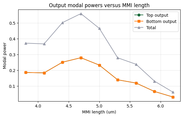
6. Sweep Visualization
The best splitter should have similar top and bottom modal powers, high total transmitted power, and low imbalance.
fig, ax = plt.subplots(figsize=(7, 4))
ax.plot(sweep_df["mmi_length_um"], sweep_df["P_top"], marker="o", label="Top output")
ax.plot(
sweep_df["mmi_length_um"], sweep_df["P_bottom"], marker="s", label="Bottom output"
)
ax.plot(sweep_df["mmi_length_um"], sweep_df["P_total"], marker="^", label="Total")
ax.set_xlabel("MMI length (um)")
ax.set_ylabel("Modal power")
ax.set_title("Output modal powers versus MMI length")
ax.grid(True, alpha=0.3)
ax.legend()
plt.show()
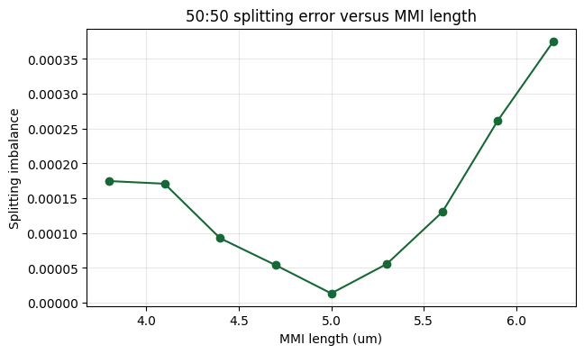
fig, ax = plt.subplots(figsize=(7, 4))
ax.plot(sweep_df["mmi_length_um"], sweep_df["imbalance"], marker="o")
ax.set_xlabel("MMI length (um)")
ax.set_ylabel("Splitting imbalance")
ax.set_title("50:50 splitting error versus MMI length")
ax.grid(True, alpha=0.3)
plt.show()
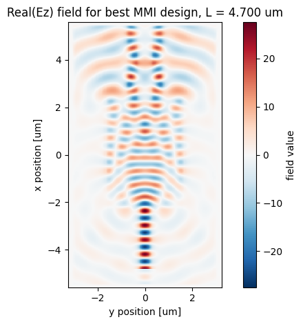
7. Field Plot for the Best Design
The selected MMI length is simulated again with a FieldMonitor. The field plot shows how the input mode expands inside the multimode region and forms two output images.
if FIELD_PNG.exists():
    print(f"Using cached field plot: {FIELD_PNG}")
    display(Image(filename=str(FIELD_PNG)))
else:
    best_sim = make_mmi_sim(
        best_length,
        min_steps_per_wvl=min_steps_per_wvl_default,
        include_field_monitor=True,
    )

    best_data = web.run(
        best_sim,
        task_name=f"best_mmi_L_{best_length:.3f}um",
        path=str(FIELD_HDF5),
        verbose=True,
    )

    field_data = best_data["field_xy"]

    # Prefer Ez for a clean scalar plot; fall back to another component if needed.
    component_name = None
    for candidate in ["Ez", "Ey", "Ex"]:
        if hasattr(field_data, candidate):
            component_name = candidate
            break

    if component_name is None:
        raise RuntimeError("No E-field component was found in the field monitor data.")

    field = (
        getattr(field_data, component_name)
        .sel(f=freq0, method="nearest")
        .real.squeeze()
    )

    fig, ax = plt.subplots()
    field.plot(ax=ax)
    ax.set_title(
        f"Real({component_name}) field for best MMI design, L = {best_length:.3f} um"
    )
    ax.set_aspect("equal")
    plt.tight_layout()
    fig.savefig(FIELD_PNG, dpi=200)
    plt.show()

print(f"Field plot path: {FIELD_PNG}")
14:42:50 -03 Created task 'best_mmi_L_4.700um' with resource_id
             'fdve-8d852204-1cb9-4bd9-931c-f003122ceca7' and task_type 'FDTD'.
             View task using web UI at
             'https://tidy3d.simulation.cloud/workbench?taskId=fdve-8d852204-1cb
             9-4bd9-931c-f003122ceca7'.
Task folder: 'default'.
Output()
14:42:53 -03 Estimated FlexCredit cost: 0.025. Minimum cost depends on task
             execution details. Use 'web.real_cost(task_id)' to get the billed
             FlexCredit cost after a simulation run.
14:42:55 -03 status = success
Output()
14:42:59 -03 Loading simulation from data_mmi_splitter/best_mmi_field.hdf5
Field plot path: data_mmi_splitter/best_mmi_field.png
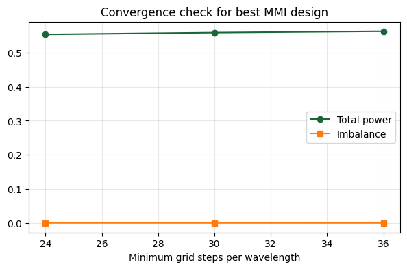
8. Short Convergence Check
To validate the result, we rerun the best design at three grid resolutions and compare the main splitter metrics.
if CONV_CSV.exists():
    print(f"Loading cached convergence results from: {CONV_CSV}")
    conv_df = pd.read_csv(CONV_CSV)
else:
    grid_values = [24, 30, 36]
    conv_sims = {
        f"grid_{grid}": make_mmi_sim(
            best_length,
            min_steps_per_wvl=grid,
            include_field_monitor=False,
        )
        for grid in grid_values
    }

    conv_batch = web.Batch(simulations=conv_sims, verbose=True)
    conv_batch_results = conv_batch.run(path_dir=str(DATA_DIR / "convergence"))

    rows = []
    for task_name in conv_batch_results.keys():
        sim_data = conv_batch_results[task_name]
        grid = int(str(task_name).replace("grid_", ""))

        p_top = extract_forward_mode_power(sim_data, "top_mode")
        p_bottom = extract_forward_mode_power(sim_data, "bottom_mode")
        metrics = score_splitter(p_top, p_bottom)

        rows.append(
            {
                "min_steps_per_wvl": grid,
                "mmi_length_um": best_length,
                **metrics,
            }
        )

    conv_df = pd.DataFrame(rows).sort_values("min_steps_per_wvl").reset_index(drop=True)
    conv_df.to_csv(CONV_CSV, index=False)
    print(f"Saved convergence results to: {CONV_CSV}")

display(conv_df)

fig, ax = plt.subplots(figsize=(7, 4))
ax.plot(
    conv_df["min_steps_per_wvl"], conv_df["P_total"], marker="o", label="Total power"
)
ax.plot(
    conv_df["min_steps_per_wvl"], conv_df["imbalance"], marker="s", label="Imbalance"
)
ax.set_xlabel("Minimum grid steps per wavelength")
ax.set_title("Convergence check for best MMI design")
ax.grid(True, alpha=0.3)
ax.legend()
plt.show()
Output()
14:43:03 -03 Started working on Batch containing 3 tasks.
14:43:09 -03 Maximum FlexCredit cost: 0.075 for the whole batch.
             Use 'Batch.real_cost()' to get the billed FlexCredit cost after
             completion.
Output()
14:43:16 -03 Batch complete.
Saved convergence results to: data_mmi_splitter/mmi_convergence_check.csv
| min_steps_per_wvl | mmi_length_um | P_top | P_bottom | P_total | imbalance | split_score | insertion_loss_dB | |
|---|---|---|---|---|---|---|---|---|
| 0 | 24 | 4.7 | 0.276801 | 0.276759 | 0.553560 | 7.636855e-05 | 0.553518 | 2.568351 |
| 1 | 30 | 4.7 | 0.279385 | 0.279355 | 0.558740 | 5.404804e-05 | 0.558710 | 2.527903 |
| 2 | 36 | 4.7 | 0.281278 | 0.281278 | 0.562555 | 1.630818e-08 | 0.562555 | 2.498349 |
9. Summary
This notebook demonstrated a compact 1×2 MMI splitter as a basic PIC and photonic-neural-network component.
The workflow included:
- a clean 2D effective-index FDTD model,
- mode-source excitation,
- modal output-power extraction,
- a length sweep for 50:50 splitting,
- field visualization for the selected design,
- a short grid-convergence check.
Notes for Further Improvement
A production-level design could extend this notebook by adding full 3D silicon-on-insulator modeling, tapered transitions, a broadband wavelength sweep, S-parameter export, and fabrication-tolerance sweeps.