Author: Donghee Lee, University of Seoul
This notebook designs a 1D dielectric phase-step grating that acts like a simple optical spatial differentiator. The FDTD result is interpreted as a physical transfer function for optical neural-network preprocessing:
$$H(k_x) \propto i k_x.$$
Here, $A_m$ is the complex transmitted amplitude of diffraction order $m$.
For the first transmitted side orders, the desired edge-detection condition is:
$$A_{+1} \approx -A_{-1}, \qquad A_0 \approx 0.$$
The notebook intentionally keeps the setup simple:
- no automatic package installation inside the notebook,
- no automatic kernel restart,
- one authentication cell,
- one simulation builder,
- one batch sweep,
- one best-field run,
- one compact convergence check.

Setup
If this is your first time using Tidy3D, please follow the Start Here guide to install the package and configure your API key.
# 1. Imports and preflight checks

from pathlib import Path

import numpy as np
import pandas as pd
import matplotlib.pyplot as plt
from IPython.display import display, Image

try:
    import tidy3d as td
except ModuleNotFoundError as exc:
    raise ModuleNotFoundError(
        "Tidy3D is not installed. Install it outside the notebook with:\n"
        "python -m pip install tidy3d==2.10.2 numpy pandas matplotlib ipython\n"
        "Then restart the kernel and run again."
    ) from exc

try:
    import tidy3d.web as web
except Exception as exc:
    raise ImportError(
        "tidy3d.web failed to import. Use a clean environment and install:\n"
        "python -m pip install tidy3d==2.10.2 numpy pandas matplotlib ipython\n"
        "Then restart the kernel and run again."
    ) from exc


# Keep public notebook output clean after the geometry has been intentionally bounded.
# The finite ridge uses a physical margin in the simulation builder; this only suppresses
# repeated non-fatal geometry warnings from cluttering the submitted notebook.
try:
    td.config.logging_level = "ERROR"
except Exception:
    import logging

    logging.getLogger("tidy3d").setLevel(logging.ERROR)

print("Tidy3D version:", td.__version__)
print("NumPy version :", np.__version__)
print("Pandas version:", pd.__version__)
print("tidy3d.web import OK")
Tidy3D version: 2.10.2
NumPy version : 2.4.4
Pandas version: 2.3.3
tidy3d.web import OK
1. Physical Parameters
The design is a one-period silicon ridge on silica. The simulation is periodic along $x$, invariant along $y$, and open along $z$. A normally incident plane wave illuminates the grating from air. Material dispersion is neglected at the design wavelength of 1.55 µm; both materials are modelled with Medium using a constant permittivity.
# Tidy3D length unit is micrometer.
um = 1.0
nm = 1e-3

# Operating wavelength.
lambda0 = 1.55 * um
freq0 = td.C_0 / lambda0
fwidth = freq0 / 30
run_time = 80 / fwidth

# Materials.
air = td.Medium(permittivity=1.0)
sio2 = td.Medium(permittivity=1.444**2)
si = td.Medium(permittivity=3.48**2)

# Grating period: choose period > wavelength so +/-1 diffraction orders propagate in air.
period = 2.20 * um

# Vertical layout.
space_above = 1.2 * lambda0
space_below = 1.2 * lambda0
substrate_thickness = 1.0 * um

# Numerical settings.
min_steps_per_wvl_default = 35
num_pml_layers = 36

# Output files.
OUT = Path("edge_detector_outputs")
OUT.mkdir(exist_ok=True)
SWEEP_CSV = OUT / "sweep_results.csv"
TOP10_CSV = OUT / "top10_submission_table.csv"
BEST_METRICS_CSV = OUT / "best_candidate_metrics.csv"
BEST_FIELD_PNG = OUT / "best_candidate_Ex_field.png"
CONVERGENCE_CSV = OUT / "convergence_check.csv"

print(f"lambda0 = {lambda0:.3f} um")
print(f"period  = {period:.3f} um")
print(f"first-order angle in air ≈ {np.degrees(np.arcsin(lambda0 / period)):.1f} deg")
lambda0 = 1.550 um
period  = 2.200 um
first-order angle in air ≈ 44.8 deg
2. Ideal Binary Phase-Step Sanity Check
An ideal half-period $\pi$-phase step suppresses the zero-order Fourier coefficient and creates strong odd diffraction orders. This analytic calculation motivates the FDTD sweep that follows: it sets the upper bound on what a real silicon ridge of finite thickness can achieve.
def binary_phase_coefficients(
    duty=0.5, phase_step=np.pi, num_harmonics=3, num_points=20001
):
    """Fourier coefficients of a one-period binary phase step."""
    x = np.linspace(-0.5, 0.5, num_points, endpoint=False)
    t = np.ones_like(x, dtype=complex)
    t[(x >= -0.5) & (x < -0.5 + duty)] = np.exp(1j * phase_step)

    coeffs = {}
    for m in range(-num_harmonics, num_harmonics + 1):
        coeffs[m] = np.mean(t * np.exp(-1j * 2 * np.pi * m * x))
    return coeffs


coeffs = binary_phase_coefficients()
for m in [-2, -1, 0, 1, 2]:
    c = coeffs[m]
    print(f"m={m:+d}: |c|^2={abs(c) ** 2:.4f}, phase={np.angle(c):+.3f} rad")

phase_diff = np.angle(coeffs[1] / coeffs[-1])
phase_error = abs(np.angle(np.exp(1j * (phase_diff - np.pi))))
print(f"phase difference A(+1)/A(-1) = {phase_diff:+.3f} rad")
print(f"error from pi phase difference = {phase_error:.3e} rad")
m=-2: |c|^2=0.0000, phase=+3.141 rad
m=-1: |c|^2=0.4053, phase=+1.571 rad
m=+0: |c|^2=0.0000, phase=+3.142 rad
m=+1: |c|^2=0.4053, phase=-1.571 rad
m=+2: |c|^2=0.0000, phase=-3.141 rad
phase difference A(+1)/A(-1) = -3.141 rad
error from pi phase difference = 1.571e-04 rad
3. Simulation Builder
The substrate uses td.inf in the periodic directions. The finite silicon ridge is intentionally kept away from the exact periodic boundary by a 1 nm margin to avoid repeated geometry warnings while preserving the intended one-period phase-step grating physics.
A normally incident PlaneWave source with a GaussianPulse excitation is placed above the grating, and two DiffractionMonitor planes record the reflected and transmitted orders. An optional FieldMonitor is attached for the best-candidate run only.
def make_simulation(
    duty=0.50,
    ridge_height=0.220,
    min_steps_per_wvl=min_steps_per_wvl_default,
    add_field_monitor=False,
):
    """Build one Tidy3D simulation for the 1D diffractive edge-detector grating."""

    # Keep the finite ridge away from the exact periodic boundary.
    # 1 nm is large enough to avoid Tidy3D boundary-touching warnings,
    # but negligible relative to the micron-scale grating period.
    edge_margin = 1e-3 * um
    ridge_width = duty * period
    ridge_width_eff = np.clip(
        ridge_width - 2 * edge_margin,
        edge_margin,
        period - 2 * edge_margin,
    )
    ridge_center_x = -period / 2 + edge_margin + ridge_width_eff / 2

    length_z = space_below + substrate_thickness + ridge_height + space_above
    z_bottom = -length_z / 2

    z_sub_center = z_bottom + space_below + substrate_thickness / 2
    z_ridge_center = z_bottom + space_below + substrate_thickness + ridge_height / 2
    z_source = (
        z_bottom + space_below + substrate_thickness + ridge_height + 0.65 * space_above
    )
    z_ref_mon = (
        z_bottom + space_below + substrate_thickness + ridge_height + 0.35 * space_above
    )
    z_trn_mon = z_bottom + 0.55 * space_below

    substrate = td.Structure(
        geometry=td.Box(
            center=(0, 0, z_sub_center),
            size=(td.inf, td.inf, substrate_thickness),
        ),
        medium=sio2,
    )

    ridge = td.Structure(
        geometry=td.Box(
            center=(ridge_center_x, 0, z_ridge_center),
            size=(ridge_width_eff, td.inf, ridge_height),
        ),
        medium=si,
    )

    source = td.PlaneWave(
        center=(0, 0, z_source),
        size=(td.inf, td.inf, 0),
        source_time=td.GaussianPulse(freq0=freq0, fwidth=fwidth),
        direction="-",
        pol_angle=0,
    )

    monitors = [
        td.DiffractionMonitor(
            center=(0, 0, z_ref_mon),
            size=(td.inf, td.inf, 0),
            freqs=[freq0],
            name="reflection",
            normal_dir="+",
        ),
        td.DiffractionMonitor(
            center=(0, 0, z_trn_mon),
            size=(td.inf, td.inf, 0),
            freqs=[freq0],
            name="transmission",
            normal_dir="-",
        ),
    ]

    if add_field_monitor:
        monitors.append(
            td.FieldMonitor(
                center=(0, 0, 0),
                size=(td.inf, 0, td.inf),
                freqs=[freq0],
                name="field_xz",
            )
        )

    boundary_spec = td.BoundarySpec(
        x=td.Boundary.periodic(),
        y=td.Boundary.periodic(),
        z=td.Boundary(
            minus=td.PML(num_layers=num_pml_layers),
            plus=td.PML(num_layers=num_pml_layers),
        ),
    )

    return td.Simulation(
        size=(period, 0, length_z),
        medium=air,
        grid_spec=td.GridSpec.auto(min_steps_per_wvl=min_steps_per_wvl),
        structures=[substrate, ridge],
        sources=[source],
        monitors=monitors,
        run_time=run_time,
        boundary_spec=boundary_spec,
    )


# Quick geometry check.
sim0 = make_simulation(duty=0.50, ridge_height=0.220)
print("Quick geometry check simulation built successfully.")
print(f"Simulation size: {sim0.size}")
print(f"Number of structures: {len(sim0.structures)}")
Quick geometry check simulation built successfully.
Simulation size: (2.2, 0.0, 4.9399999999999995)
Number of structures: 2
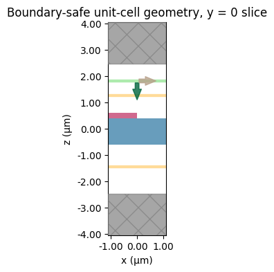
# Optional geometry plot.
fig, ax = plt.subplots(1, 1, figsize=(7, 4))
sim0.plot(y=0, ax=ax)
ax.set_title("Boundary-safe unit-cell geometry, y = 0 slice")
plt.show()
4. Diffraction-Order Objective
The score rewards strong and balanced transmitted $\pm 1$ orders, penalizes zero-order leakage, and penalizes phase deviation from $\pi$ between $A_{+1}$ and $A_{-1}$. It is a single scalar that ranks all geometries in the sweep.
def _scalar(value):
    return float(np.asarray(value).squeeze())


def phase_error_to_pi(a_plus, a_minus):
    if abs(a_plus) == 0 or abs(a_minus) == 0:
        return np.pi
    phase_diff = np.angle(a_plus / a_minus)
    return abs(np.angle(np.exp(1j * (phase_diff - np.pi))))


def diffraction_metrics(sim_data, polarization="p"):
    """Extract edge-detector metrics from a completed Tidy3D simulation."""

    trn = sim_data["transmission"]
    ref = sim_data["reflection"]

    total_power = _scalar(trn.power.sum() + ref.power.sum())

    p_m1 = _scalar(trn.power.sel(orders_x=-1, orders_y=0, f=freq0, method="nearest"))
    p_0 = _scalar(trn.power.sel(orders_x=0, orders_y=0, f=freq0, method="nearest"))
    p_p1 = _scalar(trn.power.sel(orders_x=+1, orders_y=0, f=freq0, method="nearest"))

    a_m1 = np.asarray(
        trn.amps.sel(orders_x=-1, orders_y=0, f=freq0, method="nearest").sel(
            polarization=polarization
        )
    ).squeeze()
    a_p1 = np.asarray(
        trn.amps.sel(orders_x=+1, orders_y=0, f=freq0, method="nearest").sel(
            polarization=polarization
        )
    ).squeeze()

    first_order_power = p_m1 + p_p1
    balance = 1 - abs(p_p1 - p_m1) / (first_order_power + 1e-12)
    phase_err = phase_error_to_pi(a_p1, a_m1)

    edge_score = (
        first_order_power * balance * np.exp(-((phase_err / 0.7) ** 2)) / (p_0 + 1e-3)
    )

    return {
        "P_total_R_plus_T": total_power,
        "P_T_m1": p_m1,
        "P_T_0": p_0,
        "P_T_p1": p_p1,
        "P_T_first_orders": first_order_power,
        "balance_pm1": balance,
        "phase_error_to_pi_rad": phase_err,
        "phase_error_to_pi_deg": np.degrees(phase_err),
        "edge_score": edge_score,
    }


def show_table(df, n=10, title="Top candidates"):
    cols = [
        "duty",
        "ridge_height_um",
        "edge_score",
        "P_T_m1",
        "P_T_0",
        "P_T_p1",
        "phase_error_to_pi_deg",
        "balance_pm1",
        "P_total_R_plus_T",
    ]
    table = df.sort_values("edge_score", ascending=False)[cols].head(n).copy()
    print(title)
    display(
        table.style.format(
            {
                "duty": "{:.3f}",
                "ridge_height_um": "{:.3f}",
                "edge_score": "{:.4g}",
                "P_T_m1": "{:.4f}",
                "P_T_0": "{:.4f}",
                "P_T_p1": "{:.4f}",
                "phase_error_to_pi_deg": "{:.2f}",
                "balance_pm1": "{:.3f}",
                "P_total_R_plus_T": "{:.3f}",
            }
        )
    )
    return table
duties = np.array([0.40, 0.45, 0.50, 0.55, 0.60])
ridge_heights = np.array([0.160, 0.190, 0.220, 0.250, 0.280, 0.310, 0.340])

sims = {}
metadata = {}

for duty in duties:
    for height in ridge_heights:
        name = f"duty={duty:.2f}_height={height:.3f}um"
        sims[name] = make_simulation(duty=float(duty), ridge_height=float(height))
        metadata[name] = {"duty": float(duty), "ridge_height_um": float(height)}

print(f"Prepared {len(sims)} simulations.")
Prepared 35 simulations.
if SWEEP_CSV.exists():
    df = pd.read_csv(SWEEP_CSV)
    print(f"Loaded cached sweep results from {SWEEP_CSV}")
else:
    print("Submitting FDTD sweep...")
    batch = web.Batch(simulations=sims, verbose=True)
    batch_results = batch.run(path_dir=str(OUT / "tidy3d_sweep_data"))

    rows = []
    for name, sim_data in batch_results.items():
        row = dict(metadata[name])
        row.update(diffraction_metrics(sim_data, polarization="p"))
        rows.append(row)

    df = (
        pd.DataFrame(rows)
        .sort_values("edge_score", ascending=False)
        .reset_index(drop=True)
    )
    df.to_csv(SWEEP_CSV, index=False)
    print(f"Saved sweep results to {SWEEP_CSV}")

print(f"Result rows: {len(df)}")
Submitting FDTD sweep...
Output()
14:42:09 -03 Started working on Batch containing 35 tasks.
14:43:03 -03 Maximum FlexCredit cost: 0.875 for the whole batch.
             Use 'Batch.real_cost()' to get the billed FlexCredit cost after
             completion.
Output()
14:44:35 -03 Batch complete.
Saved sweep results to edge_detector_outputs/sweep_results.csv
Result rows: 35
top10 = show_table(df, n=10, title="Submission table: top FDTD candidates")
top10.to_csv(TOP10_CSV, index=False)
print(f"Saved top-10 table to {TOP10_CSV}")
Submission table: top FDTD candidates
| duty | ridge_height_um | edge_score | P_T_m1 | P_T_0 | P_T_p1 | phase_error_to_pi_deg | balance_pm1 | P_total_R_plus_T | |
|---|---|---|---|---|---|---|---|---|---|
| 0 | 0.400 | 0.310 | 0.0009286 | 0.3776 | 0.0027 | 0.3783 | 140.68 | 0.999 | 0.994 |
| 1 | 0.400 | 0.340 | 0.0001049 | 0.3537 | 0.0293 | 0.3548 | 140.73 | 0.998 | 0.994 |
| 2 | 0.600 | 0.310 | 7.395e-05 | 0.3497 | 0.0148 | 0.3503 | 146.28 | 0.999 | 0.993 |
| 3 | 0.600 | 0.340 | 5.54e-05 | 0.3410 | 0.0197 | 0.3413 | 146.25 | 1.000 | 0.992 |
| 4 | 0.600 | 0.280 | 3.717e-05 | 0.3787 | 0.0328 | 0.3795 | 146.32 | 0.999 | 0.993 |
| 5 | 0.600 | 0.250 | 1.129e-05 | 0.3981 | 0.1152 | 0.3995 | 146.35 | 0.998 | 0.993 |
| 6 | 0.400 | 0.280 | 9.175e-06 | 0.2508 | 0.2543 | 0.2517 | 140.51 | 0.998 | 0.997 |
| 7 | 0.450 | 0.280 | 6.722e-06 | 0.4046 | 0.0171 | 0.4055 | 158.97 | 0.999 | 0.993 |
| 8 | 0.400 | 0.220 | 6.313e-06 | 0.2112 | 0.2987 | 0.2115 | 140.75 | 0.999 | 0.998 |
| 9 | 0.450 | 0.310 | 5.068e-06 | 0.3620 | 0.0205 | 0.3634 | 158.97 | 0.998 | 0.993 |
Saved top-10 table to edge_detector_outputs/top10_submission_table.csv
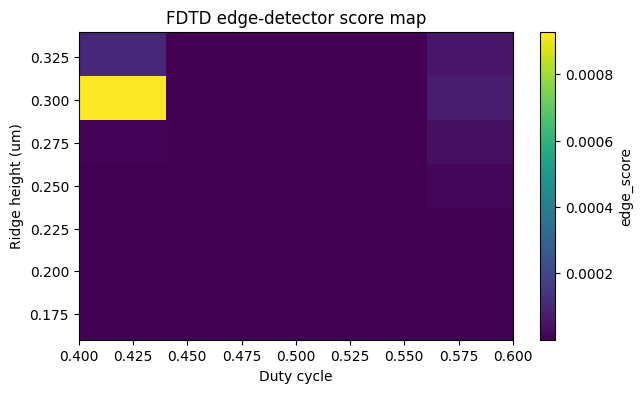
pivot = df.pivot(index="ridge_height_um", columns="duty", values="edge_score")

fig, ax = plt.subplots(1, 1, figsize=(7, 4))
im = ax.imshow(
    pivot.values,
    origin="lower",
    aspect="auto",
    extent=[duties.min(), duties.max(), ridge_heights.min(), ridge_heights.max()],
)
ax.set_xlabel("Duty cycle")
ax.set_ylabel("Ridge height (um)")
ax.set_title("FDTD edge-detector score map")
plt.colorbar(im, ax=ax, label="edge_score")
plt.show()

best = df.sort_values("edge_score", ascending=False).iloc[0]
print("Best candidate:")
display(best.to_frame().T)
Best candidate:
| duty | ridge_height_um | P_total_R_plus_T | P_T_m1 | P_T_0 | P_T_p1 | P_T_first_orders | balance_pm1 | phase_error_to_pi_rad | phase_error_to_pi_deg | edge_score | |
|---|---|---|---|---|---|---|---|---|---|---|---|
| 0 | 0.4 | 0.31 | 0.99383 | 0.377636 | 0.00269 | 0.378256 | 0.755891 | 0.99918 | 2.455331 | 140.680092 | 0.000929 |
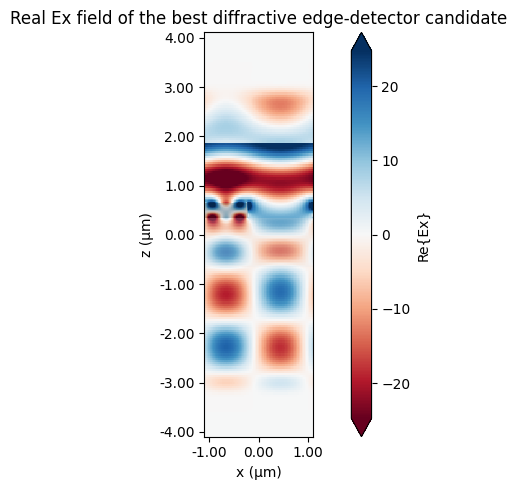
6. Best-Candidate Field Plot
The best design is rerun with an $x$-$z$ FieldMonitor so the spatial structure of the diffracted field can be visualized. The result is cached as a PNG and CSV.
if BEST_METRICS_CSV.exists() and BEST_FIELD_PNG.exists():
    best_metrics = pd.read_csv(BEST_METRICS_CSV)
    print(f"Loaded cached best-candidate metrics from {BEST_METRICS_CSV}")
    show_table(best_metrics, n=1, title="Best candidate with field monitor")
    display(Image(filename=str(BEST_FIELD_PNG)))
else:
    best = df.sort_values("edge_score", ascending=False).iloc[0]

    sim_best = make_simulation(
        duty=float(best["duty"]),
        ridge_height=float(best["ridge_height_um"]),
        add_field_monitor=True,
    )

    sim_best_data = web.run(
        sim_best,
        task_name="FDTD_diffractive_edge_detector_best_field",
        path=str(OUT / "best_field_data.hdf5"),
        verbose=True,
    )

    best_metrics = pd.DataFrame(
        [
            {
                "duty": float(best["duty"]),
                "ridge_height_um": float(best["ridge_height_um"]),
                **diffraction_metrics(sim_best_data, polarization="p"),
            }
        ]
    )
    best_metrics.to_csv(BEST_METRICS_CSV, index=False)

    show_table(best_metrics, n=1, title="Best candidate with field monitor")

    fig, ax = plt.subplots(1, 1, figsize=(8, 5))
    sim_best_data.plot_field("field_xz", field_name="Ex", val="real", f=freq0, ax=ax)
    ax.set_title("Real Ex field of the best diffractive edge-detector candidate")
    fig.tight_layout()
    fig.savefig(BEST_FIELD_PNG, dpi=200, bbox_inches="tight")
    plt.show()

    print(f"Saved best metrics to {BEST_METRICS_CSV}")
    print(f"Saved field plot to {BEST_FIELD_PNG}")
14:45:23 -03 Created task 'FDTD_diffractive_edge_detector_best_field' with
             resource_id 'fdve-308fad43-a539-4f89-b47c-c7a47ea0507f' and
             task_type 'FDTD'.
             View task using web UI at
             'https://tidy3d.simulation.cloud/workbench?taskId=fdve-308fad43-a53
             9-4f89-b47c-c7a47ea0507f'.
Task folder: 'default'.
Output()
14:45:26 -03 Estimated FlexCredit cost: 0.025. Minimum cost depends on task
             execution details. Use 'web.real_cost(task_id)' to get the billed
             FlexCredit cost after a simulation run.
14:45:28 -03 status = success
Output()
14:45:32 -03 Loading simulation from edge_detector_outputs/best_field_data.hdf5
Best candidate with field monitor
| duty | ridge_height_um | edge_score | P_T_m1 | P_T_0 | P_T_p1 | phase_error_to_pi_deg | balance_pm1 | P_total_R_plus_T | |
|---|---|---|---|---|---|---|---|---|---|
| 0 | 0.400 | 0.310 | 0.0009286 | 0.3776 | 0.0027 | 0.3783 | 140.68 | 0.999 | 0.994 |
Saved best metrics to edge_detector_outputs/best_candidate_metrics.csv
Saved field plot to edge_detector_outputs/best_candidate_Ex_field.png
7. Compact Convergence Check
The best geometry is rerun at min_steps_per_wvl = 30, 40, 50 to confirm that the key diffraction metrics are stable under grid refinement.
convergence_steps = [30, 40, 50]

if CONVERGENCE_CSV.exists():
    conv_df = pd.read_csv(CONVERGENCE_CSV)
    print(f"Loaded cached convergence check from {CONVERGENCE_CSV}")
else:
    best = df.sort_values("edge_score", ascending=False).iloc[0]
    duty_best = float(best["duty"])
    height_best = float(best["ridge_height_um"])

    conv_sims = {}
    conv_metadata = {}

    for steps in convergence_steps:
        name = f"best_min_steps_per_wvl={steps}"
        conv_sims[name] = make_simulation(
            duty=duty_best,
            ridge_height=height_best,
            min_steps_per_wvl=steps,
        )
        conv_metadata[name] = {
            "min_steps_per_wvl": steps,
            "duty": duty_best,
            "ridge_height_um": height_best,
        }

    print(f"Submitting {len(conv_sims)} convergence simulations...")
    conv_batch = web.Batch(simulations=conv_sims, verbose=True)
    conv_results = conv_batch.run(path_dir=str(OUT / "tidy3d_convergence_data"))

    rows = []
    for name, sim_data in conv_results.items():
        row = dict(conv_metadata[name])
        row.update(diffraction_metrics(sim_data, polarization="p"))
        rows.append(row)

    conv_df = pd.DataFrame(rows).sort_values("min_steps_per_wvl").reset_index(drop=True)

    ref = conv_df.iloc[-1]
    for col in ["edge_score", "P_T_m1", "P_T_0", "P_T_p1", "phase_error_to_pi_deg"]:
        conv_df[f"{col}_rel_change_vs_50_pct"] = (
            100 * (conv_df[col] - ref[col]) / (abs(ref[col]) + 1e-12)
        )

    conv_df.to_csv(CONVERGENCE_CSV, index=False)
    print(f"Saved convergence check to {CONVERGENCE_CSV}")

cols = [
    "min_steps_per_wvl",
    "edge_score",
    "P_T_m1",
    "P_T_0",
    "P_T_p1",
    "phase_error_to_pi_deg",
    "edge_score_rel_change_vs_50_pct",
    "P_T_0_rel_change_vs_50_pct",
    "phase_error_to_pi_deg_rel_change_vs_50_pct",
]

display(
    conv_df[cols].style.format(
        {
            "edge_score": "{:.4g}",
            "P_T_m1": "{:.4f}",
            "P_T_0": "{:.4f}",
            "P_T_p1": "{:.4f}",
            "phase_error_to_pi_deg": "{:.2f}",
            "edge_score_rel_change_vs_50_pct": "{:+.2f}%",
            "P_T_0_rel_change_vs_50_pct": "{:+.2f}%",
            "phase_error_to_pi_deg_rel_change_vs_50_pct": "{:+.2f}%",
        }
    )
)
Output()
Submitting 3 convergence simulations...
14:45:36 -03 Started working on Batch containing 3 tasks.
14:45:41 -03 Maximum FlexCredit cost: 0.075 for the whole batch.
             Use 'Batch.real_cost()' to get the billed FlexCredit cost after
             completion.
Output()
14:45:49 -03 Batch complete.
Saved convergence check to edge_detector_outputs/convergence_check.csv
| min_steps_per_wvl | edge_score | P_T_m1 | P_T_0 | P_T_p1 | phase_error_to_pi_deg | edge_score_rel_change_vs_50_pct | P_T_0_rel_change_vs_50_pct | phase_error_to_pi_deg_rel_change_vs_50_pct | |
|---|---|---|---|---|---|---|---|---|---|
| 0 | 30 | 0.0009675 | 0.3769 | 0.0028 | 0.3772 | 140.20 | +16.67% | +11.48% | -0.96% |
| 1 | 40 | 0.0008864 | 0.3782 | 0.0027 | 0.3788 | 141.01 | +6.89% | +3.95% | -0.39% |
| 2 | 50 | 0.0008293 | 0.3790 | 0.0026 | 0.3797 | 141.56 | +0.00% | +0.00% | +0.00% |
8. Conclusion
The notebook demonstrates that a single-layer silicon phase-step grating on silica can implement a compact 1D optical edge detector at 1.55 µm. The FDTD sweep identifies a duty cycle and ridge height that maximize the balanced $\pm 1$ transmitted orders while suppressing the zero order, and the convergence check shows the result is robust to grid refinement.
For further reading, see the DiffractionMonitor API and the related Multilevel blazed diffraction grating example.