Author: Zhiyi Yuan, Nanyang Technological University
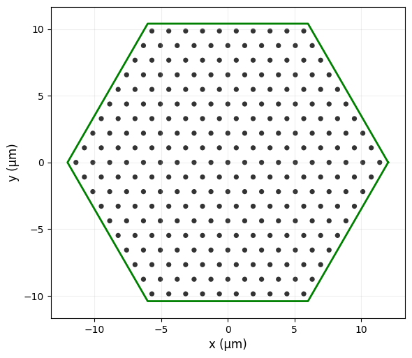
In this notebook, we create an open Dirac cavity as a hexagonal photonic crystal and analyze its spectrum and resonance properties.

[1]:
from os.path import join
import matplotlib.pyplot as plt
import numpy as np
import tidy3d as td
from tidy3d import web
from tidy3d.plugins.resonance import ResonanceFinder
09:58:43 EST WARNING: Configuration found in legacy location '~/.tidy3d'.
             Consider running 'tidy3d config migrate'.
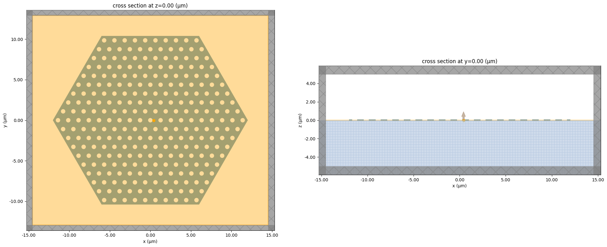
Create structure
[2]:
a = 1.265
r = 0.272
t_slab = 0.2
n_side = 10
L = n_side - 0.5
Lx = 2*(L+2)*a
Ly = 2*(L*np.sqrt(3)/2+2)*a
x0, y0, z0 = 0.0, 0.0, 0.0
medium_hole = td.Medium(permittivity=1.0)        # holes (air)
medium_slab = td.Medium(permittivity=3.4**2)     # slab
axis = 2
def open_dirac_cavity():
    vertices = [
        ( L*a, 0.0),
        ( L*a/2,  L*np.sqrt(3)*a/2),
        (-L*a/2,  L*np.sqrt(3)*a/2),
        (-L*a, 0.0),
        (-L*a/2, -L*np.sqrt(3)*a/2),
        ( L*a/2, -L*np.sqrt(3)*a/2),
    ]

    slab_structure = td.Structure(
        geometry=td.PolySlab(
            slab_bounds=(z0 - t_slab/2, z0 + t_slab/2),
            vertices=vertices,
        ),
        medium=medium_slab,
        name="slab_polyslab",
    )
    cylinders = []
    for i in range(1, n_side + 1):  # hexagon side length
        center_x, center_y = x0 + (i - 1) * a, y0
        for j in range(0, 6 - 5 * (i == 1)):  # iterate through hexagon sides
            for _ in range(0, i - 1 + (i == 1)):  # iterate along each hexagon side
                if i > 1:
                    center_x += a * np.cos(2*np.pi/3 + j*np.pi/3)
                    center_y += a * np.sin(2*np.pi/3 + j*np.pi/3)
                cylinders.append(
                    td.Cylinder(
                        axis=axis,
                        radius=r,
                        center=(center_x, center_y, z0),
                        length=t_slab,
                    )
                )
    holes_structure = td.Structure(
        geometry=td.GeometryGroup(geometries=cylinders),
        medium=medium_hole,
        name="holes_cylinders",
    )
    return [slab_structure, holes_structure]
structures = open_dirac_cavity()
slab = structures[0]  # 显式赋值slab变量 - Explicitly assign slab variable
holes = structures[1] # 显式赋值holes变量 - Explicitly assign holes variable
#print(f"介质层结构:{structures[0].name}")
#print(f"孔阵列结构:{structures[1].name}")
print(f"holes number:{len(structures[1].geometry.geometries)}")
holes number:271
[3]:
fig, ax = plt.subplots(figsize=(6, 6))
vertices = np.array(slab.geometry.vertices)
vertices_closed = np.vstack([vertices, vertices[0]])  # 闭合多边形 - Close the polygon
ax.plot(vertices_closed[:,0], vertices_closed[:,1], "g-", lw=2)
hole_centers_x = []  # 所有孔的x坐标 - x coordinates of all holes
hole_centers_y = []  # 所有孔的y坐标 - y coordinates of all holes
for cyl in holes.geometry.geometries:
    center = cyl.center
    hole_centers_x.append(center[0])
    hole_centers_y.append(center[1])
ax.scatter(
    hole_centers_x,
    hole_centers_y,
    s=cyl.radius * 100,
    c="black",
    marker="o",
    edgecolors="none",
    alpha=0.8,
)
ax.set_aspect("equal")
ax.set_xlabel("x (μm)", fontsize=12)
ax.set_ylabel("y (μm)", fontsize=12)
ax.tick_params(axis='both', labelsize=10)
ax.grid(alpha=0.2)
x_min = vertices[:,0].min() - a
x_max = vertices[:,0].max() + a
y_min = vertices[:,1].min() - a
y_max = vertices[:,1].max() + a
ax.set_xlim(x_min, x_max)
ax.set_ylim(y_min, y_max)
plt.tight_layout()
plt.show()
Create simulation
[4]:
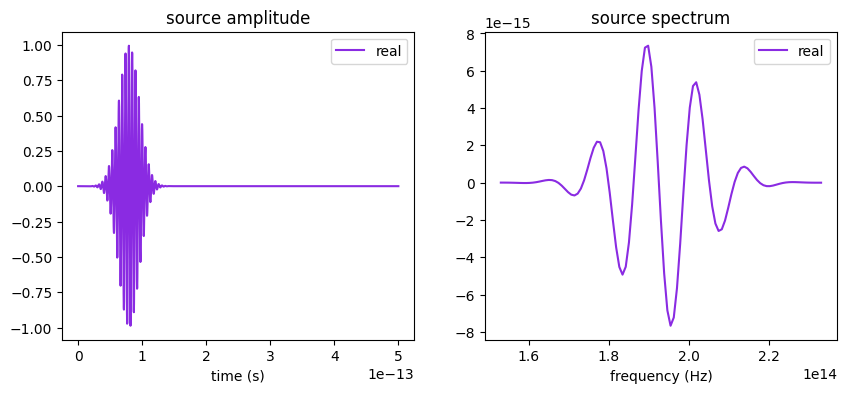
# Source frequency and width
freq0 = 192.5e12   # 200THz
fwidth = 10e12
runTime = 20e-12

# Source: plot time dependence to verify when the source pulse decayed
source = td.PointDipole(
    center=(a/2-a/6, 0, 0),
    source_time=td.GaussianPulse(freq0=freq0, fwidth=fwidth),
    polarization="Hz",
)
sources = [source]
fig, ax = plt.subplots(1, 2, figsize=(10, 4))
source.source_time.plot(np.linspace(0, 5e-13, 2000), ax=ax[0])
source.source_time.plot_spectrum(times=np.linspace(0, 5e-13, 2000), ax=ax[1])
plt.show()
[5]:
# Time series monitor for Q-factor computation
time_series = td.FieldTimeMonitor(
    center=[a/2-a/6, 0, 0], size=[0, 0, 0], start=2e-13, name="time_series"
)
# near field
field_near = td.FieldMonitor(
    center=[0, 0, 0],
    size=[Lx, Ly, 0],
    freqs = np.linspace(187.5e12, 197.5e12, 101),
    name="field_near",
    apodization=td.ApodizationSpec(start=3e-12, width=2e-13),
)
# far field fft
#ux = np.linspace(-1,1,101)
#uy = np.linspace(-1,1,101)
#field_far_fft = td.FieldProjectionKSpaceMonitor(
#    center=(0, 0, t_slab/2 + 0.1),
#    size=(Lx, Ly, 0),
#    freqs = np.linspace(185e12, 200e12, 76),
#    name="field_far_fft",
#    proj_axis=2,
#    ux=ux,
#    uy=uy,
#    apodization=td.ApodizationSpec(start=2e-13, width=2e-13),
#)
[6]:
# Suppress warnings for some of the holes being too close to the PML
td.config.logging.level = "ERROR"
# Mesh step in x, y, z, in microns
steps_per_unit_length = 20
grid_spec = td.GridSpec(
    grid_x=td.UniformGrid(dl=a / steps_per_unit_length),
    grid_y=td.UniformGrid(dl=a / steps_per_unit_length * np.sqrt(3) / 2),
    grid_z=td.AutoGrid(min_steps_per_wvl=steps_per_unit_length),
)
# Simulation
size_z = 10
sim_size = [Lx, Ly, size_z]
sim = td.Simulation(
    size=sim_size,
    grid_spec=grid_spec,
    structures=structures,
    sources=sources,
    monitors=[time_series, field_near],
    run_time=runTime,
    boundary_spec=td.BoundarySpec.all_sides(boundary=td.PML()),
    symmetry=(0, 0, 1),
    shutoff=1e-5,
)
[7]:
fig, ax = plt.subplots(1, 2, figsize=(20, 8))
sim.plot(z=0, ax=ax[0])
#sim.plot_grid(z=0, ax=ax[0], color="blue", alpha=0.3, linewidth=0.5)
ax[0].set_aspect("equal")
sim.plot(y=0, ax=ax[1])
ax[1].set_aspect("equal")
plt.tight_layout()
plt.show()
Run simulation
[8]:
from tidy3d import web
# Create a job and upload it
job = web.Job(simulation=sim, task_name="Open_Dirac_Cavity", verbose=True)
# Estimate its maximum cost before running
estimated_cost = web.estimate_cost(job.task_id)
print(f"Estimated maximum cost: {estimated_cost:.3f} FlexCredits")
09:58:45 EST Created task 'Open_Dirac_Cavity' with resource_id
             'fdve-678b6329-5709-489e-a4ca-a9957308305d' and task_type 'FDTD'.
             View task using web UI at
             'https://tidy3d.simulation.cloud/workbench?taskId=fdve-678b6329-570
             9-489e-a4ca-a9957308305d'.
Task folder: 'default'.
Output()
09:58:47 EST Estimated FlexCredit cost: 2.095. Minimum cost depends on task
             execution details. Use 'web.real_cost(task_id)' to get the billed
             FlexCredit cost after a simulation run.
09:58:48 EST Estimated FlexCredit cost: 2.095. Minimum cost depends on task
             execution details. Use 'web.real_cost(task_id)' to get the billed
             FlexCredit cost after a simulation run.
Estimated maximum cost: 2.095 FlexCredits
[9]:
sim_data = web.run(sim, task_name="Open_Dirac_Cavity", path="Dirac_Cavity_V2.hdf5",verbose=True)
             Created task 'Open_Dirac_Cavity' with resource_id
             'fdve-6ac4c5b0-515f-420e-9f31-209f45f33352' and task_type 'FDTD'.
             View task using web UI at
             'https://tidy3d.simulation.cloud/workbench?taskId=fdve-6ac4c5b0-515
             f-420e-9f31-209f45f33352'.
Task folder: 'default'.
Output()
09:58:50 EST Estimated FlexCredit cost: 2.095. Minimum cost depends on task
             execution details. Use 'web.real_cost(task_id)' to get the billed
             FlexCredit cost after a simulation run.
09:58:51 EST status = queued
             To cancel the simulation, use 'web.abort(task_id)' or
             'web.delete(task_id)' or abort/delete the task in the web UI.
             Terminating the Python script will not stop the job running on the
             cloud.
Output()
09:58:59 EST starting up solver
running solver
Output()
10:00:12 EST early shutoff detected at 32%, exiting.
10:00:13 EST status = postprocess
Output()
10:00:35 EST status = success
10:00:37 EST View simulation result at
             'https://tidy3d.simulation.cloud/workbench?taskId=fdve-6ac4c5b0-515
             f-420e-9f31-209f45f33352'.
Output()
10:01:42 EST Loading simulation from Dirac_Cavity_V2.hdf5
Analyze spectrum
[10]:
sim_data = td.SimulationData.from_file("Dirac_Cavity_V2.hdf5")
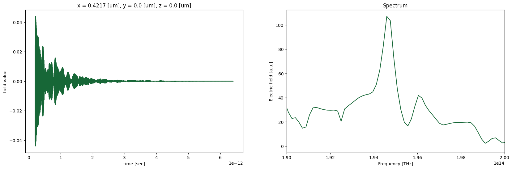
[11]:
# Get data from the TimeMonitor
tdata = sim_data["time_series"]
time_series = tdata.Hz.squeeze()
fig, (ax1, ax2) = plt.subplots(1, 2, figsize=(20, 6))
# Plot time dependence
time_series.plot(ax=ax1)
# Make frequency mesh and plot spectrum
dt = sim_data.simulation.dt
fmesh = np.linspace(-1 / dt / 2, 1 / dt / 2, time_series.size)
spectrum = np.fft.fftshift(np.fft.fft(time_series))
ax2.plot(fmesh, np.abs(spectrum))
ax2.set_xlim(190e12,200e12)
ax2.set_xlabel("Frequency [THz]")
ax2.set_ylabel("Electric field [a.u.]")
ax2.set_title("Spectrum")
plt.show()
Analyze resonance data
[12]:
resonance_finder = ResonanceFinder(freq_window=(187.5e12, 195e12), init_num_freqs=100)
resonance_data = resonance_finder.run(sim_data["time_series"])
resonance_data.to_dataframe()
[12]:
| decay | Q | amplitude | phase | error | |
|---|---|---|---|---|---|
| freq | |||||
| 1.866466e+14 | 3.219630e+12 | 182.122663 | 0.244486 | -1.841334 | 0.000703 |
| 1.875533e+14 | 5.032551e+12 | 117.080987 | 0.391330 | 2.544543 | 0.001288 |
| 1.877141e+14 | 1.036471e+12 | 568.970173 | 0.016556 | 3.028083 | 0.000217 |
| 1.893997e+14 | 1.783065e+12 | 333.704424 | 0.202839 | 1.745468 | 0.000383 |
| 1.909463e+14 | 1.815567e+12 | 330.406590 | 0.336411 | 1.265731 | 0.000293 |
| 1.945941e+14 | 1.505145e+12 | 406.163921 | 0.240529 | -1.918391 | 0.000169 |
| 1.947196e+14 | 3.297701e+12 | 185.501860 | 0.130286 | 0.123704 | 0.001281 |
| 1.959386e+14 | 2.605625e+12 | 236.242390 | 0.125737 | -1.974891 | 0.000624 |
| 1.972617e+14 | 3.434281e+12 | 180.449943 | 0.104981 | 3.109832 | 0.001481 |
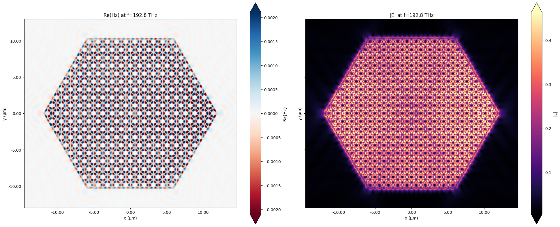
[13]:
freq_hz = 192.8e12
freq_thz = freq_hz / 1e12
fig, (ax1, ax2) = plt.subplots(1, 2, figsize=(20, 8), sharex=True, sharey=True)
sim_data.plot_field("field_near", "Hz", val="real", z=0, f=freq_hz, ax=ax1, eps_alpha=0.1)
ax1.set_title(f"Re(Hz) at f={freq_thz:.1f} THz")
sim_data.plot_field("field_near", "E", val="abs", z=0, f=freq_hz, ax=ax2, eps_alpha=0.1)
ax2.set_title(f"|E| at f={freq_thz:.1f} THz")
plt.tight_layout()
plt.show()
[ ]: