Author: Yankun (Alex) Meng, Duke University
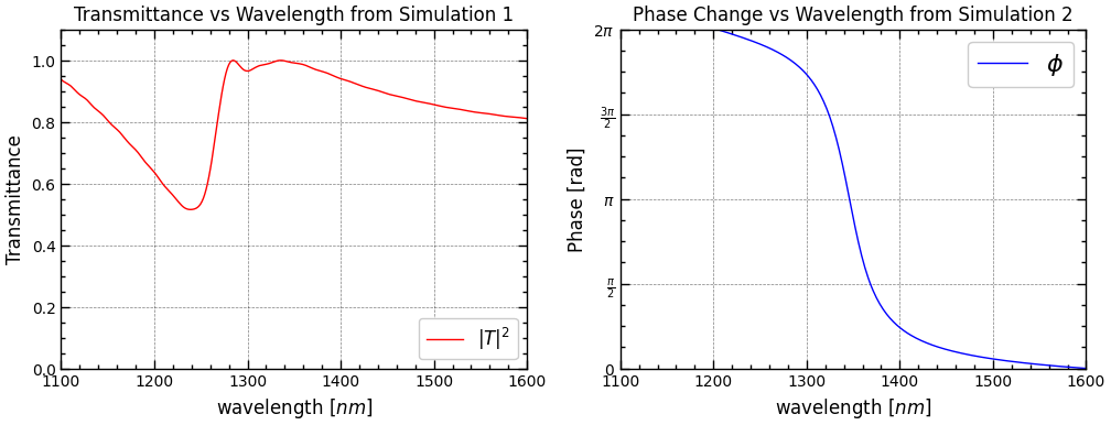
Dielectric Huygens' metasurfaces exploit the overlap of electric and magnetic dipole resonances in high-index nanoparticles to achieve near-unity transmittance with full 2π phase coverage. In this notebook we reproduce the transmittance and phase spectra from Figures 5(a) and 5(c) of the reference below, and perform a mesh convergence study using Tidy3D.
We follow: M. Decker, I. Staude, M. Falkner, J. Dominguez, D. N. Neshev, I. Brener, T. Pertsch, and Y. S. Kivshar, "High-Efficiency Dielectric Huygens' Surfaces," Advanced Optical Materials, vol. 3, no. 6, pp. 813–820, 2015, doi: 10.1002/adom.201400584.
Imports and Simulation Overview
import matplotlib.pyplot as plt
import numpy as np
import tidy3d as td
import tidy3d.web as web
import scienceplots

td.config.logging_level = "ERROR"
Initialization
We define the simulation components following a systematic workflow.
The simulation is built in seven steps:
- Frequency Range Specification
- Computational Domain Size
- Grid Specifications (Discretization size)
- Structures and Materials
- Sources
- Monitors
- Run time
- Boundary Condition Specification
0 Frequency Range Specification
# 0 Define a FreqRange object with desired wavelengths
fr = td.FreqRange.from_wvl_interval(wvl_min=1.1, wvl_max=1.6)
N = 301
lda0 = td.C_0 / fr.freq0
1 Computational Domain Size
# 1 Computational Domain Size
h = 0.220  # Height of cylinder
spc = 2
Lz = spc + h + h + spc

P = 0.666  # periodicity
sim_size = [P, P, Lz]
2 Grid Resolution
Grid resolution is uniform grid in the horizontal direction with a yee cell length of $\frac{P}{32}$ where $P$ is the periodicity. In the vertical direction, AutoGrid means it's non-uniform and adjusted based on the wavelength of the particular medium. Here, min_steps_per_wvl=32 means we are taking a minimum of 32 steps based on the wavelength, which will be shorter in the medium with a higher index of refraction.
dl = P / 32
horizontal_grid = td.UniformGrid(dl=dl)
vertical_grid = td.AutoGrid(min_steps_per_wvl=32)
grid_spec=td.GridSpec(
    grid_x=horizontal_grid,
    grid_y=horizontal_grid,
    grid_z=vertical_grid,
)
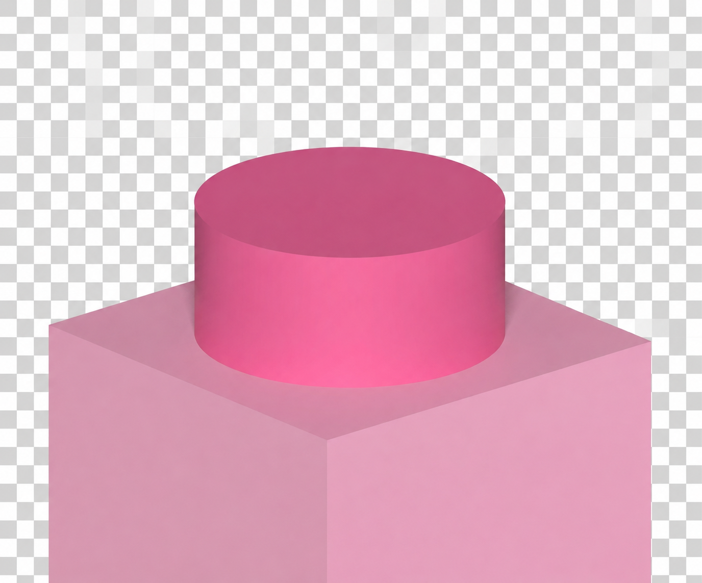
3 Structures and Materials
Structures and Materials for the meta-atom
r = 0.242  # radius of the cylinder
n_Si = 3.5
Si = td.Medium(permittivity=n_Si**2, name='Si')
cylinder = td.Structure(
    geometry=td.Cylinder(center=[0, 0, h / 2], radius=r, length=h, axis=2), medium=Si
)
Background Medium for Figure 5(a) ($n_1=1.4, n_2=1.45$)
# Background medium for the first simulation
n_glass = 1.4
n_SiO2 = 1.45
glass = td.Medium(permittivity=n_glass**2, name='glass')
SiO2 = td.Medium(permittivity=n_SiO2**2, name='oxide')

substrate = td.Structure(
    geometry=td.Box(
        center=(0,0,-Lz/2),
        size=(td.inf,td.inf,2 * (spc+h))
    ),
    medium=SiO2,
    name='substrate'
)

glass = td.Structure(
    geometry=td.Box(
        center=(0,0,Lz/2),
        size=(td.inf,td.inf,2 * (spc+h))
    ),
    medium=glass,
    name='superstrate'
)
Background Medium for Figure 5(c) ($n=1.66$)
# Background medium for the second simulation
# Polymer
n_polymer = 1.66
polymer = td.Structure(
    geometry=td.Box(
        center=(0,0,0),
        size=(td.inf,td.inf,td.inf)
    ),
    medium=td.Medium(permittivity=n_polymer**2, name='polymer'),
    name='polymer'
)
4 The Source
The source is a simple Plane wave that traverses in the -z axis, placed $\frac{\lambda_0}{2}$ distance above the metaatom in the computational domain. Polarization is along the x-axis, that's what pol_angle=0 means.
source = td.PlaneWave(
    source_time=fr.to_gaussian_pulse(),
    size=(td.inf, td.inf, 0),
    center=(0, 0, Lz/2 - spc + 0.5 * lda0),
    direction="-",
    pol_angle=0
)
5 Monitors
Monitor for Transmittance
flux_monitor = td.FluxMonitor(
    center=(0, 0, -Lz/2 + spc - 0.5 * lda0),
    size=(td.inf, td.inf, 0),
    freqs=fr.freqs(N),
    name="flux_monitor"
)
Monitor for Phase
# We use FieldMonitor instead of DiffractionMonitor because
# DiffractionMonitor only gives you amplitudes of diffraction orders,
# losing phase detail if you care about continuous phase.
field_monitor = td.FieldMonitor(
    center=(0, 0, -Lz/2 + spc - 0.5 * lda0),
    size=(td.inf, td.inf, 0),
    fields=["Ex"],
    freqs=fr.freqs(N),
    name="field_monitor"
)
6 Run Time
bandwidth = fr.fmax - fr.fmin
run_time_short = 50 / bandwidth # run_time for the transmittance simulation
run_time_long = 200 / bandwidth # run_time for the phase simulation
7 Boundary Conditions
We apply PML in the +z and -z boundaries.
bc = td.BoundarySpec(
    x=td.Boundary.periodic(),
    y=td.Boundary.periodic(),
    z=td.Boundary.pml()
)
Helper Function
A helper function is used to create both the "actual" (with the cylinder) and "norm" (without the cylinder) simulations, following the DRY Principle.
The function builds a pair of Tidy3D simulations—one with and one without the meta-atom—so that the normalised transmittance or phase can be obtained by dividing the two results.
def simulation_helper(background, monitors, run_time):
sim_empty=td.Simulation(
size=sim_size,
grid_spec=grid_spec,
structures=background,
sources=[source],
monitors=monitors,
run_time=run_time,
boundary_spec=bc
)
background.append(cylinder)
sim_actual = td.Simulation(
size=sim_size,
grid_spec=grid_spec,
structures=background,
sources=[source],
monitors=monitors,
run_time=run_time,
boundary_spec=bc
)
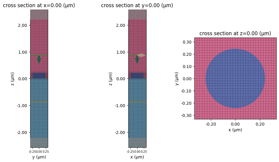
# Always visualize simulation before running
fig, (ax1,ax2,ax3) = plt.subplots(1, 3, figsize=(12, 6))
ax1.tick_params(axis='x', labelsize=7)
ax2.tick_params(axis='x', labelsize=7)
sim_actual.plot(x=0, ax=ax1)
sim_actual.plot_grid(x=0, ax=ax1)
sim_actual.plot(y=0, ax=ax2)
sim_actual.plot_grid(y=0, ax=ax2)
sim_actual.plot(z=0, ax=ax3)
sim_actual.plot_grid(z=0, ax=ax3)
plt.savefig(f'huygens_structure_{background[0].name}.png', dpi=300)
plt.show()
sims = {
"norm": sim_empty,
"actual": sim_actual,
}
return sims
Transmittance Simulation
sims = simulation_helper(
    background=[substrate, glass],
    monitors=[flux_monitor],
    run_time=run_time_short
)
batch = web.Batch(simulations=sims, verbose=True)
batch_data = batch.run(path_dir="data/huygens5a")
Output()
13:18:43 EDT Started working on Batch containing 2 tasks.
13:18:45 EDT Maximum FlexCredit cost: 0.050 for the whole batch.
             Use 'Batch.real_cost()' to get the billed FlexCredit cost after
             completion.
Output()
Batch complete.
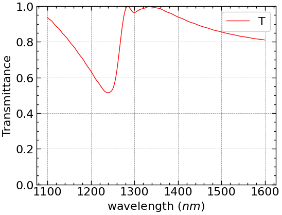
Transmittance Results
# this uses scienceplots to make plots look better
plt.style.use(['science', 'notebook', 'grid'])
T = batch_data["actual"]["flux_monitor"].flux / batch_data["norm"]["flux_monitor"].flux
# plot transmission, compare to paper results, look similar
fig, ax = plt.subplots(1, 1, figsize=(6, 4.5))
plt.plot(td.C_0 / fr.freqs(N) * 1000, np.abs(T)**2, "r", lw=1, label="T")
plt.xlabel(r"wavelength ($nm$)")
plt.ylabel("Transmittance")
plt.ylim(0, 1)
plt.legend()
plt.show()
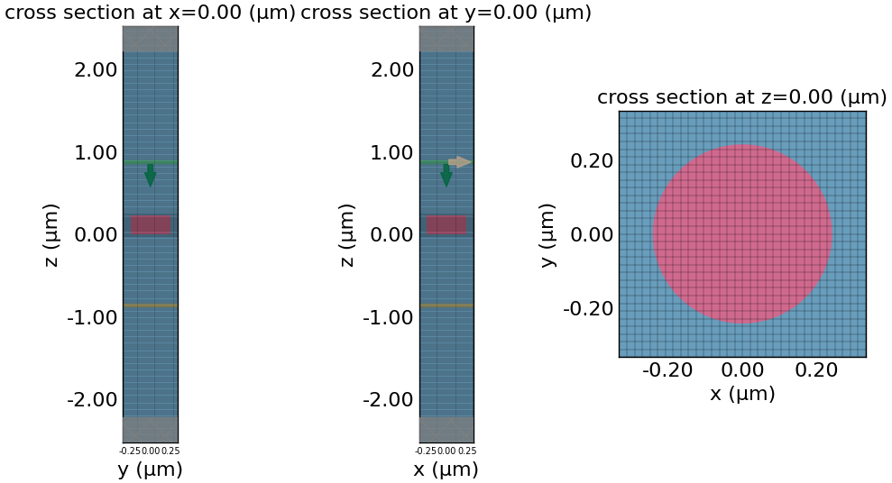
Phase Simulation
sims = simulation_helper(
    background=[polymer],
    monitors=[field_monitor],
    run_time=run_time_long
)
batch = web.Batch(simulations=sims, verbose=True)
batch_data = batch.run(path_dir="data/huygens5c")
Output()
13:18:49 EDT Started working on Batch containing 2 tasks.
13:18:51 EDT Maximum FlexCredit cost: 0.050 for the whole batch.
             Use 'Batch.real_cost()' to get the billed FlexCredit cost after
             completion.
Output()
Batch complete.
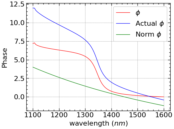
Phase Results
# Data Extraction
Ex_actual = batch_data["actual"]["field_monitor"].Ex
Ex_norm = batch_data["norm"]["field_monitor"].Ex
Ex = Ex_actual / Ex_norm
# 1. Compute average over the xy-plane
Ex_avg = np.mean(Ex[:, :, 0, :], axis=(0,1))

# 2. Compute phase
phase_avg = np.angle(Ex_avg)

# 3. Unwrap phase to remove ±pi jumps
phase_avg_unwrapped = np.unwrap(phase_avg)

# 4. Make relative to first point (optional)
phase_rel = phase_avg_unwrapped - phase_avg_unwrapped[0]

phase_actual = np.unwrap(np.angle(np.mean(Ex_actual[:, :, 0, :], axis=(0,1))))
phase_norm = np.unwrap(np.angle(np.mean(Ex_norm[:, :, 0, :], axis=(0,1))))
fig, ax = plt.subplots(1, 1, figsize=(6, 4.5))
plt.plot(td.C_0 / fr.freqs(N) * 1000, phase_rel, "r", lw=1, label="$\phi$")
plt.plot(td.C_0 / fr.freqs(N) * 1000, phase_actual, "b", lw=1, label="Actual $\phi$")
plt.plot(td.C_0 / fr.freqs(N) * 1000, phase_norm, "g", lw=1, label="Norm $\phi$")
plt.xlabel(r"wavelength ($nm$)")
plt.ylabel("Phase")
plt.legend()
plt.show()
Final Plotting
fig, axes = plt.subplots(1, 2, figsize=(12, 4))

# work on the first figure
ax = axes[0]
ax.tick_params(axis="both", labelsize=10)
ax.plot(td.C_0 / fr.freqs(N) * 1000, np.abs(T)**2, "r", lw=1, label="$|T|^2$")
ax.set_xlabel(r"wavelength [$nm$]", fontsize=12)
ax.set_ylabel("Transmittance", fontsize=12)
ax.set_title("Transmittance vs Wavelength from Simulation 1", fontsize=12)
ax.set_xlim(1100, 1600)
ax.set_ylim(0, 1.1)
ax.legend(loc="lower right", fontsize=12)

# work on the second figure
ax = axes[1]
ax.tick_params(axis="both", labelsize=10)
ax.plot(td.C_0 / fr.freqs(N) * 1000, phase_rel, "b", lw=1, label="$\phi$")
ax.set_xlabel(r"wavelength [$nm$]", fontsize=12)
ax.set_ylabel("Phase [rad]", fontsize=12)
ax.set_title("Phase Change vs Wavelength from Simulation 2", fontsize=12)
ax.set_xlim(1100, 1600)
ax.set_ylim(0, np.pi*2)
yticks = [0, np.pi/2, np.pi, 3*np.pi/2, 2*np.pi]
ytick_labels = [r"$0$", r"$\frac{\pi}{2}$", r"$\pi$",
                r"$\frac{3\pi}{2}$", r"$2\pi$"]
ax.set_yticks(yticks)
ax.set_yticklabels(ytick_labels)
ax.legend()

plt.savefig("huygens.png", dpi=300)
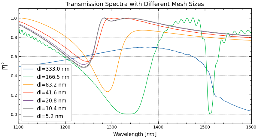
Mesh Study
Here, we set out to study the effect of different yee cell length on the transmittance.
dls = [P/2, P/4, P/8, P/16, P/32, P/64, P/128] # mesh study list
sims = {}
# for each dl in dls
for i, dl in enumerate(dls):
    # 2 Grid Specifications
    horizontal_grid = td.UniformGrid(dl=dl)
    vertical_grid = td.AutoGrid(min_steps_per_wvl=32)
    grid_spec=td.GridSpec(
        grid_x=horizontal_grid,
        grid_y=horizontal_grid,
        grid_z=vertical_grid,
    )

    # 4 Sources
    source = td.PlaneWave(
        source_time=fr.to_gaussian_pulse(),
        size=(td.inf, td.inf, 0),
        center=(0, 0, Lz/2 - spc + 2 * dl),
        direction="-",
        pol_angle=0
    )

    # 5 Monitor
    monitor = td.FluxMonitor(
        center=(0, 0, -Lz/2 + spc - 2*dl),
        size=(td.inf, td.inf, 0),
        freqs=fr.freqs(N),
        name="flux"
    )

    sim_empty=td.Simulation(
        size=sim_size,
        grid_spec=grid_spec,
        structures=[substrate, glass],
        sources=[source],
        monitors=[monitor],
        run_time=run_time_short,
        boundary_spec=bc
    )

    sim_actual = td.Simulation(
        size=sim_size,
        grid_spec=grid_spec,
        structures=[substrate, glass, cylinder],
        sources=[source],
        monitors=[monitor],
        run_time=run_time_short,
        boundary_spec=bc
    )

    sims[f"norm{i}"] = sim_empty
    sims[f"actual{i}"] = sim_actual
# verify the sims dictionary
print(sims.keys())
batch = web.Batch(simulations=sims, verbose=True)
dict_keys(['norm0', 'actual0', 'norm1', 'actual1', 'norm2', 'actual2', 'norm3', 'actual3', 'norm4', 'actual4', 'norm5', 'actual5', 'norm6', 'actual6'])
# run the simulations
batch_data = batch.run(path_dir="data")
Output()
13:18:57 EDT Started working on Batch containing 14 tasks.
13:19:10 EDT Maximum FlexCredit cost: 0.392 for the whole batch.
             Use 'Batch.real_cost()' to get the billed FlexCredit cost after
             completion.
Output()
13:19:13 EDT Batch complete.
Mesh Study Results
# Extract results
x = td.C_0 / fr.freqs(N) * 1000
Ts = []
for i in range(len(dls)):
    Ts.append(batch_data[f"actual{i}"]["flux"].flux / batch_data[f"norm{i}"]["flux"].flux)
# Plot results
plt.figure(figsize=(10, 5))
for i, T in enumerate(Ts):
    plt.plot(x, np.abs(T)**2, "-",lw=1, label=f"dl={dls[i] * 1000:.1f} nm")
plt.xlabel(r"Wavelength [$nm$]", fontsize=12)
plt.ylabel(r"$|T|^2$", fontsize=12)
plt.xlim(1100, 1600)
plt.ylim(-0.1, 1.1)
plt.legend(fontsize=12)
plt.tick_params(axis='both', labelsize=10) # change tick label size to 10
plt.title("Transmission Spectra with Different Mesh Sizes", fontsize=14)
plt.savefig("mesh_convergence.png", dpi=300)
plt.show()