Author: Yankun (Alex) Meng, Duke University
Dielectric metasurfaces supporting quasi-bound states in the continuum (q-BICs) can produce ultrasharp resonances with high quality factors by introducing a symmetry-breaking coupler into the unit cell. In this notebook, we use Tidy3D's ResonanceFinder plugin to locate q-BIC resonances in a GaP elliptical-pillar metasurface and then compute the near-field enhancement at the resonance frequency.
We reproduce and extend results from G. Q. Moretti, A. Tittl, E. Cortés, S. A. Maier, A. V. Bragas, and G. Grinblat, "Introducing a Symmetry-Breaking Coupler into a Dielectric Metasurface Enables Robust High-Q Quasi-BICs," Advanced Photonics Research, vol. 3, no. 12, p. 2200111, 2022, doi: 10.1002/adpr.202200111. Specifically, we obtain the field enhancement profile for the middle configuration in Figure S2 of the supplemental.

Imports and Utilities
import matplotlib.pyplot as plt
from pathlib import Path
from tidy3d import web
import pandas as pd
import tidy3d as td
import numpy as np
import time
class SimRunner:
    """
    Handles running, monitoring, and loading results of multiple Tidy3D simulations.
    """
    def __init__(self, sims):
        """
        Initialize with a dictionary of simulations.
        sims: dict where keys are simulation names and values are td.Simulation objects
        """
        self.sims = sims or {}
        print(f"Received Simulations: {self.sims.keys()}")
        self.results = None

    def add_simulation(self, name, sim):
        """Add a single simulation to the runner."""
        self.sims[name] = sim

    def run(self, name):
        if self.results is not None:
            return self.results
        start = time.perf_counter()
        path = Path(name)
        results = None

        if not path.exists():
            if self.sims is None:
                print("No simulations provided.")
                elapsed = time.perf_counter() - start
                print(f"run() took {elapsed:.2f} seconds")
                return None
            batch = web.Batch(simulations=self.sims, verbose=True)
            batch.upload()
            batch.estimate_cost()
            user_input = input("Press Enter to continue...Type Any Character to STOP RUNNING.")
            if user_input == "":
                def run(batch, name):
                    batch.start()
                    batch.monitor()
                    return batch.load(name)
                results = run(batch, name)
            else:
                print("Terminated Run.")
                elapsed = time.perf_counter() - start
                print(f"run() took {elapsed:.2f} seconds")
                print(f"Real Cost: {batch.real_cost()}")
                return None
        else:
            print(f"Loading existing results: {name}")
            batch = web.Batch.from_file(f"{name}/batch.hdf5")
            results = batch.load(path_dir=name, replace_existing=True)

        elapsed = time.perf_counter() - start
        print(f"run() took {elapsed:.2f} seconds")
        print(f"Real Cost: {batch.real_cost()}")
        self.results = results
        return results
1. Set the Geometry
Simulation Parameters
Define the wavelength range and derive the frequency parameters used throughout the notebook.
# Unit conversion
nm = 1e-3

# Simulation parameters
lam1 = 970*nm        # Beginning Wavelength
lam2 = 980*nm        # Ending Wavelength
n = 1001             # Number of Points to Sample

# Derived Quantities
freqs = np.linspace(td.C_0 / lam2, td.C_0 / lam1, n) # Sampled Frequency Points
freq0 = freqs[len(freqs)//2]                         # Central Frequency
freqw = np.max(freqs) - np.min(freqs)                # Frequency bandwidth
Geometries
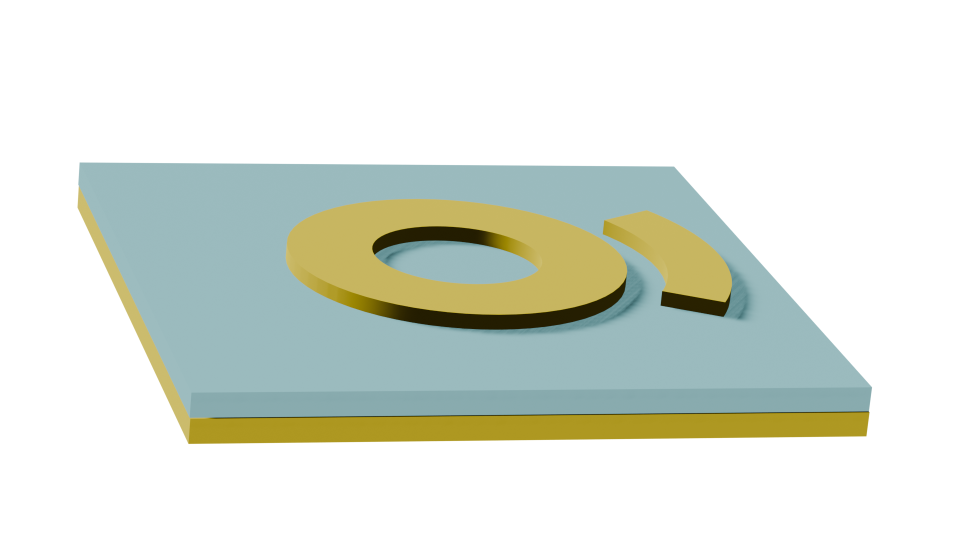
Define the unit cell dimensions, meta-atom parameters, and material properties. The metasurface consists of two GaP elliptical pillars and a cylindrical symmetry-breaking coupler on a glass substrate.
# Unit Cell Definition
Px = Py = 600 * nm                     # Periodicity
height = 200 * nm                      # Height of the metaatoms
thick_air = 1                          # Spacing Above metaatom to the top PML
thick_sub = 1 + height                 # Thickness of the substrate
Lz = thick_sub + height + thick_air    # Distance from bottom PML to Top PML
sim_size = (Px, Py, Lz)                # Simulation Size Definition

# -----------------------------------------------------
# PML  |    thick_sub | height | thick_air      |  PML
# -----------------------------------------------------

# Metaatom Dimensions
d = 300 * nm                # Distance between main pillars
a = 380 * nm                # Major axis Diameter
b = 170 * nm                # Minor axis Diameter
w = 300 * nm                # Y-Distance from center of main pillars to bottom symmetry point
coupler_diameter = 80*nm    # coupler's diameter
delta_y = 200*nm            # coupler's distance from bottom symmetry point
y_offset = 100*nm           # the Y-displacement of all metaatoms in the unit cell
left_x = -d/2
right_x = d/2


# Mediums
Glass = td.Medium(permittivity=2.25)
gap =  td.Sellmeier.from_dispersion(n=3.1908, dn_dwvl=-0.21978, freq=freq0)
Structures
Create the Tidy3D structures for the elliptical pillars, the symmetry-breaking coupler, and the glass substrate.
left = td.Structure(
    geometry=td.Cylinder(
        center=(left_x, 0, height/2),
        radius=b / 2,
        length=height,
        axis=2
    ).scaled(x=1, y=a/b, z=1)
    .rotated(angle=-0*(np.pi/180), axis=2)
    .translated(x=0, y=y_offset, z=0),
    medium=gap
)

right = td.Structure(
    geometry=td.Cylinder(
        center=(right_x, 0, height/2),
        radius=b / 2,
        length=height,
        axis=2
    ).scaled(x=1, y=a/b, z=1)
    .rotated(angle=0*(np.pi/180), axis=2)
    .translated(x=0, y=y_offset, z=0),
    medium=gap
)

coupler = td.Structure(
    geometry=td.Cylinder(
        center=(0, -w + delta_y + y_offset, height/2),
        radius=coupler_diameter / 2,
        length=height,
        axis=2
    ),
    medium=gap
)

# substrate
substrate = td.Structure(
    geometry=td.Box(
        center=(0,0,-Lz / 2),
        size=(td.inf,td.inf,Lz)
    ),
    medium=Glass,
    name='substrate'
)
structures = [left, right, coupler, substrate]
2. Resonance Finder
We use the ResonanceFinder plugin to extract resonance frequencies and Q factors from time-domain field signals via harmonic inversion. Randomly placed point dipole sources excite all supported modes of the structure.
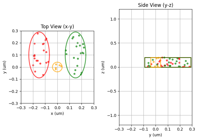
1. Place Sources
Place randomly positioned Ex-polarized point dipoles inside each meta-atom to broadly excite the resonant modes of the structure.
rng = np.random.default_rng(11)
def generate_random_points(center_x, center_y, N, a = a/2, b = b/2, height = height):
    # Random polar coordinates
    theta = rng.uniform(0, 2*np.pi, N)
    r = np.sqrt(rng.uniform(0, 1, N))  # uniform area

    # Map to ellipse
    x_points = r * b * np.cos(theta) + center_x
    y_points = r * a * np.sin(theta) + center_y
    z_points = rng.uniform(0, height, N)
    return list(zip(x_points, y_points, z_points))
# ----- Generate points for each structure -----
left_points = generate_random_points(center_x=left_x, center_y=y_offset, N=20)
right_points = generate_random_points(center_x=right_x, center_y=y_offset, N=20)
center_points = generate_random_points(center_x=0, center_y=-w + delta_y + y_offset, N=5,
                                       a=coupler_diameter/2, b=coupler_diameter/2)

# Flatten all points for Tidy3D
dip_positions = left_points + right_points + center_points
num_dipoles = len(dip_positions)

# Random phases for dipoles
dip_phases = rng.uniform(0, 2*np.pi, num_dipoles)

# ----- Create dipoles -----
dipoles = []
for i in range(num_dipoles):
    pulse = td.GaussianPulse(freq0=freq0, fwidth=freqw, phase=dip_phases[i])
    dipoles.append(
        td.PointDipole(
            source_time=pulse,
            center=dip_positions[i],
            polarization="Ex",
            name=f"dip_source_{i}",
        )
    )
sources = dipoles
fig, (ax1, ax2) = plt.subplots(1, 2, figsize=(7,5), tight_layout=True)

# Structure parameters for plotting
structures_plotting = [
    (left_points, left_x, y_offset, a/2, b/2, 'red'),
    (right_points, right_x, y_offset, a/2, b/2, 'green'),
    (center_points, 0, -w + delta_y + y_offset, coupler_diameter/2, coupler_diameter/2, 'orange')
]

theta_outline = np.linspace(0, 2*np.pi, 500)

# ----- Top view (x-y) -----
for pts, cx, cy, aa, bb, color in structures_plotting:
    xs, ys, zs = zip(*pts)
    ax1.scatter(xs, ys, color=color, s=15, alpha=0.6)
    # Ellipse outline
    x_ellipse = bb * np.cos(theta_outline) + cx
    y_ellipse = aa * np.sin(theta_outline) + cy
    ax1.plot(x_ellipse, y_ellipse, color=color, linewidth=2, alpha=0.7)
ax1.set_xlim(-Px/2, Px/2)
ax1.set_ylim(-Py/2, Py/2)
ax1.set_aspect('equal')
ax1.set_title("Top View (x-y)")
ax1.set_xlabel("x (um)")
ax1.set_ylabel("y (um)")
ax1.grid(True)

# ----- Side view (y-z) -----
for pts, cx, cy, aa, bb, color in structures_plotting:
    xs, ys, zs = zip(*pts)
    ax2.scatter(ys, zs, color=color, s=15, alpha=0.6)
    # Side rectangle
    ax2.plot([cy - aa, cy + aa, cy + aa, cy - aa, cy - aa],
                [0, 0, height, height, 0],
                color=color, linewidth=2, alpha=0.7)
ax2.set_xlim(-Py/2, Py/2)
ax2.set_ylim(-Lz/2, Lz/2)
ax2.set_aspect('auto')
ax2.set_title("Side View (y-z)")
ax2.set_xlabel("y (um)")
ax2.set_ylabel("z (um)")
ax2.grid(True)
2. Place Monitors
Set up FieldTimeMonitor objects to record the time-domain signals needed by the ResonanceFinder.
run_time = 20/freqw # this is a hyperparameter
t_start = 2/freqw # time monitor starts measuring
print(run_time)
print(t_start)

# Set z at halfway of the metaatoms
z=height/2

# Initialization
mon_positions = [
    (left_x, y_offset - a/3, z),
    (left_x, y_offset + a/3, z),
    (left_x, y_offset, z),
    (right_x,y_offset - a/3, z),
    (right_x,y_offset + a/3, z),
    (right_x,y_offset, z),
    (0, -w + delta_y + y_offset, z), # coupler center
    (left_x, y_offset - a/2 - 0.01, z),
    (right_x, y_offset - a/2 - 0.01, z),
]


# Loop Assignment
monitors_time = []
for i in range(len(mon_positions)):
    monitors_time.append(
        td.FieldTimeMonitor(
            fields=["Ex"],
            center=tuple(mon_positions[i]),
            size=(0, 0, 0),
            start=t_start,
            name="monitor_time_" + str(i),
        )
    )

# This Monitors the z-cut xy plane of all the metaatoms
fieldZ = td.FieldMonitor(
    center=[0, 0, height /2],
    size=[td.inf, td.inf, 0],
    freqs=[freq0],
    name="z"
)

# This monitors the x-cut yz plane of the right metaatom
fieldY = td.FieldMonitor(
    center=[d/2, 0, 0],
    size=[0, td.inf, 0.8],
    freqs=[freq0],
    name="y"
)

monitors = [fieldZ, fieldY]
monitors.extend(monitors_time)
6.341720577907208e-12
6.341720577907208e-13
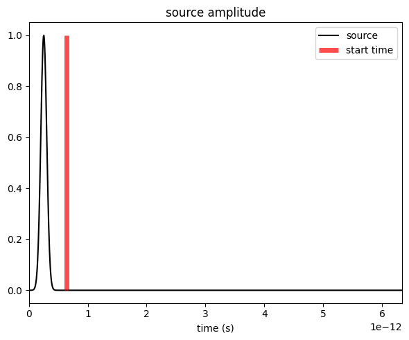
fig, ax = plt.subplots(tight_layout=True, figsize=(6, 5))

plot_time = run_time
sources[0].source_time.plot(times=np.linspace(0, plot_time, 1001), val="abs", ax=ax)

ax.set_xlim(0, plot_time)
ax.vlines(t_start, 0, 1, linewidth=5, color="r", alpha=0.7)
ax.legend(["source", "start time"])
plt.show()
3. The Mesh
Use the automatic nonuniform meshing with 32 steps per wavelength to accurately resolve the high-Q resonance.
grid_spec = td.GridSpec.auto(min_steps_per_wvl=32)
4. Simulation
Assemble the simulation with periodic boundaries in the x and y directions and PML in the z direction.
sim = td.Simulation(
    size=sim_size,
    grid_spec=grid_spec,
    structures=structures,
    sources=sources,
    monitors=monitors,
    boundary_spec=td.BoundarySpec(
        x=td.Boundary.periodic(), y=td.Boundary.periodic(), z=td.Boundary.pml()
    ),
    run_time=run_time,
)
sim.plot_3d()
sims = {"sim": sim}
runner = SimRunner(sims)
res = runner.run("rf")
Received Simulations: dict_keys(['sim'])
Loading existing results: rf
Output()
run() took 7.75 seconds
11:16:55 EDT Total billed flex credit cost: 0.084.
Real Cost: 0.08418566594261809
sim_data = res["sim"]
             WARNING: Simulation final field decay value of 0.00943 is greater
             than the simulation shutoff threshold of 1e-05. Consider running
             the simulation again with a larger 'run_time' duration for more
             accurate results.
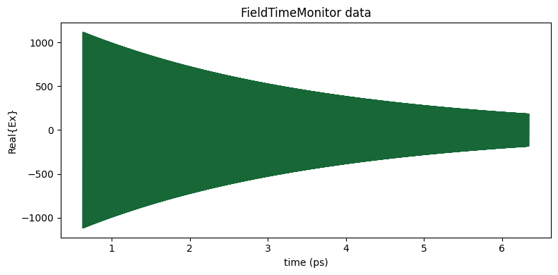
fig, ax1 = plt.subplots(1, 1, tight_layout=True, figsize=(8, 4))

ax1.plot(
    sim_data.monitor_data["monitor_time_0"].Ex.t * 1e12,
    np.real(sim_data.monitor_data["monitor_time_0"].Ex.squeeze()),
)
ax1.set_title("FieldTimeMonitor data")
ax1.set_xlabel("time (ps)")
ax1.set_ylabel("Real{Ex}")
plt.show()
from tidy3d.plugins.resonance import ResonanceFinder

resonance_finder = ResonanceFinder(
    freq_window=(freqs[0], freqs[-1])
)
# Exclude the frequency domain field monitors
field_time_signals = [
    data for data in sim_data.data
    if hasattr(data, "monitor") and data.monitor.type == "FieldTimeMonitor"
]
# while running this line of code, your computer will slow down because it utilizes your cpu resources
resonance_data = resonance_finder.run(signals=field_time_signals)
df = resonance_data.to_dataframe()
df.to_csv("output.csv")
3. Field Enhancement
Using the resonance frequency and Q factor from Part 2, we now set up a broadband plane-wave simulation to compute the transmittance and near-field enhancement of the metasurface at the q-BIC resonance.
1. Simulation Parameters
We have to use simulation parameters derived from the resonance finder.
resonance_data = pd.read_csv("output.csv")

# Unit conversion
nm = 1e-3

# resonance data
fr = resonance_data.freq
Q = resonance_data.Q

# linewidth
df = fr / Q

# choose pulse bandwidth multiplier
mult = 10

# final frequency width
fwidth = mult * df

# frequency bounds
fmin = fr - fwidth/2
fmax = fr + fwidth/2

# convert to wavelength bounds
lam1 = (td.C_0 / fmax).values[0]
lam2 = (td.C_0 / fmin).values[0]
# Unit conversion
nm = 1e-3

# Simulation parameters
n = 701             # Number of Points to Sample

# Derived Quantities
freqs = np.linspace(td.C_0 / lam2, td.C_0 / lam1, n) # Sampled Frequency Points
freq0 = freqs[len(freqs)//2]                         # Central Frequency
lda0 = td.constants.C_0 / freq0                      # Central Wavelength
freqw = np.max(freqs) - np.min(freqs)                # Frequency bandwidth
monitor_wvls = td.C_0 / freqs                        # Wavelengths to Monitor (used for plotting convenience)
print("="*70)
print(f"{'BASIC SIMULATION SETUP':^65}")
print("="*70)
print(f"{'[monitor_wvls] Wavelength array':<40}: {np.min(monitor_wvls*1000):.2f} nm to {np.max(monitor_wvls*1000):.2f} nm")
print(f"{'[freqs] Frequency array':<40}: {np.min(freqs):.4e} Hz to {np.max(freqs):.4e} Hz")
print(f"{'[n] Number of points':<40}: {n}")
print(f"{'[freq0] Central Frequency':<40}: {freq0:.6e} Hz")
print(f"{'[freqw] Bandwidth':<40}: {freqw:.6e} Hz")
print(f"{'[lda0]  Central λ':<40}: {lda0*1000:.2f} nm")
print(f"{'[run_time] Simulation run time':<40}: {run_time:.6e} sec")
print("="*70 + "\n")
======================================================================
                     BASIC SIMULATION SETUP
======================================================================
[monitor_wvls] Wavelength array         : 974.74 nm to 977.96 nm
[freqs] Frequency array                 : 3.0655e+14 Hz to 3.0756e+14 Hz
[n] Number of points                    : 701
[freq0] Central Frequency               : 3.070563e+14 Hz
[freqw] Bandwidth                       : 1.012808e+12 Hz
[lda0]  Central λ                       : 976.34 nm
[run_time] Simulation run time          : 6.341721e-12 sec
======================================================================
2. Sources and Monitors
Define a single x-polarized plane wave source and frequency-domain monitors for the transmittance and field profiles.
# This is the plane wave source
source = td.PlaneWave(
    source_time=td.GaussianPulse(
        freq0=freq0,
        fwidth=freqw
    ),
    size=(td.inf, td.inf, 0),
    center=(0, 0, height + thick_air / 2),
    direction="-",
    pol_angle=0
)

# this monitors the transmittance
t_monitor = td.FluxMonitor(
    center=(0, 0, - Lz / 4),
    size=(td.inf, td.inf, 0),
    freqs=freqs,
    name="t",
    normal_dir="-"
)

# This Monitors the z-cut xy plane of all the metaatoms
fieldZ = td.FieldMonitor(
    center=[0, 0, height /2],
    size=[td.inf, td.inf, 0],
    freqs=freqs,
    name="z"
)

# This monitors the x-cut yz plane of the right metaatom
fieldY = td.FieldMonitor(
    center=[d/2, 0, 0],
    size=[0, td.inf, 0.8],
    freqs=freqs,
    name="y"
)

sources = [source]
monitors = [t_monitor, fieldZ, fieldY]
3. The Run Time
Compute the simulation run time from the resonance Q factor to ensure sufficient field decay.
# decay time
tau = (Q / (np.pi * fr)).values[0]

# recommended simulation runtime
run_time = 5 * tau

print(f"Decay time tau: {tau*1e12:.2f} ps")
print(f"Recommended simulation run time: {run_time *1e12:.2f} ps")
Decay time tau: 3.14 ps
Recommended simulation run time: 15.71 ps
4. The Simulation
Assemble the field enhancement simulation and a reference simulation without structures for normalization.
sim = td.Simulation(
    size=sim_size,
    grid_spec=grid_spec,
    structures=structures,
    sources=sources,
    monitors=monitors,
    boundary_spec=td.BoundarySpec(
        x=td.Boundary.periodic(), y=td.Boundary.periodic(), z=td.Boundary.pml()
    ),
    run_time=run_time,
)

sim_ref = sim.copy(update={"structures": []})
sim.plot_3d()
min_grid_x = np.min(np.diff(sim.grid.boundaries.x))
min_grid_y = np.min(np.diff(sim.grid.boundaries.y))
min_grid_z = np.min(np.diff(sim.grid.boundaries.z))
min_grid = np.min([min_grid_x, min_grid_y, min_grid_z])

print(f"minimal grid size in x is {min_grid_x}.")
print(f"minimal grid size in y is {min_grid_y}.")
print(f"minimal grid size in z is {min_grid_z}.")
print(f"minimal grid {min_grid}")
minimal grid size in x is 0.008333333333333304.
minimal grid size in y is 0.004999999999999671.
minimal grid size in z is 0.00952380952380949.
minimal grid 0.004999999999999671
C = 0.99                            # Default Courant Factor
dt = C*min_grid / td.C_0
times=np.arange(0, run_time, dt)
print(len(times))
951719
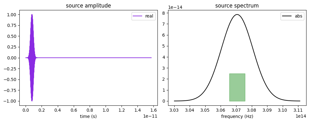
def plot_source(source, run_time, times, freqs=None, xlim_time=None, xlim_freq=None, save_as=None, dpi=300):
    f, (ax1, ax2) = plt.subplots(1, 2, tight_layout=True, figsize=(10, 4))
    ax1 = source.source_time.plot(times, ax=ax1)
    if xlim_time is not None: ax1.set_xlim(xlim_time)

    ax2 = source.source_time.plot_spectrum(times, val='abs', ax=ax2)
    if freqs is not None: ax2.fill_between([np.min(freqs), np.max(freqs)], [-0e-16, -0e-16], [2.5e-14, 2.5e-14], alpha=0.4, color='g')
    if xlim_freq is not None: ax2.set_xlim(xlim_freq)
    if save_as:
        Path(save_as).parent.mkdir(parents=True, exist_ok=True)  # creates all missing folders
        plt.savefig(save_as, dpi=dpi)
    plt.show()

plot_source(sim.sources[0], run_time, times, freqs=freqs)
sims = {"sim": sim,
        "sim_ref": sim_ref}
runner = SimRunner(sims)
res_2 = runner.run("Broadband-02")
Received Simulations: dict_keys(['sim', 'sim_ref'])
Loading existing results: Broadband-02
Output()
run() took 11.55 seconds
11:17:11 EDT Total billed flex credit cost: 0.176.
Real Cost: 0.17609205061187852
simData = res_2["sim"]
simData_ref = res_2["sim_ref"]
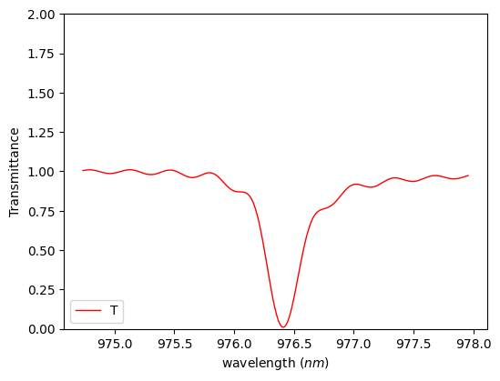
Plotting the Transmittance
Extract and plot the transmittance spectrum. The sharp dip indicates the high-Q q-BIC resonance.
# Extract the Transmittance
# "t" was the name of the flux monitor defined when defining monitors
T = simData["t"].flux
fig, ax = plt.subplots(1, 1, figsize=(6, 4.5))
plt.plot(monitor_wvls * 1000, T, color="red", lw=1, label="T")
plt.xlabel(r"wavelength ($nm$)")
plt.ylabel("Transmittance")
plt.legend(loc="lower left", fontsize=10)
plt.savefig("T.png", dpi=300)
plt.ylim(0, 2)
plt.show()
Plotting the Field Enhancement
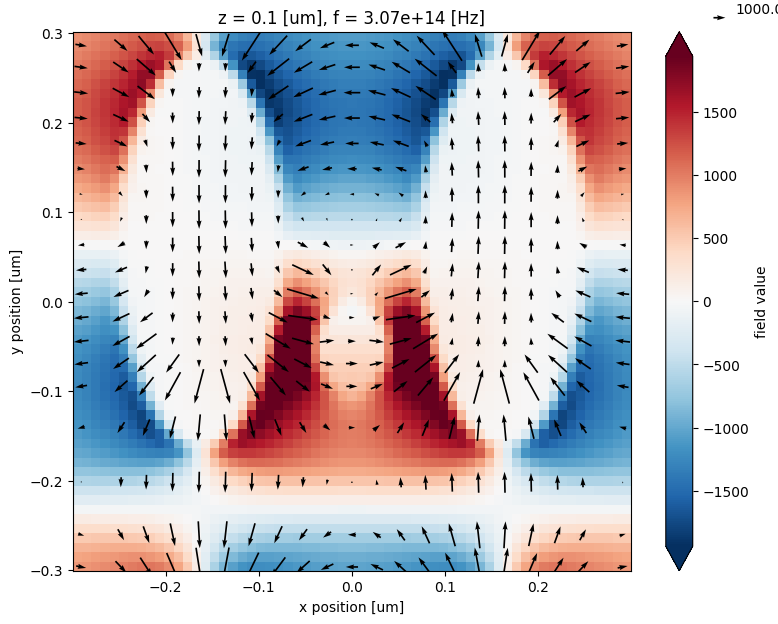
Visualize the electric field distribution at the resonance frequency and compute the field enhancement by normalizing to the reference (empty) simulation.
field_ds_z = simData.at_centers("z")
field_ds_y = simData.at_centers("y")
             WARNING: Colocating data that has already been colocated during the
             solver run. For most accurate results when colocating to custom
             coordinates set 'Monitor.colocate' to 'False' to use the raw data
             on the Yee grid and avoid double interpolation. Note: the default
             value was changed to 'True' in Tidy3D version 2.4.0.
11:17:12 EDT WARNING: Colocating data that has already been colocated during the
             solver run. For most accurate results when colocating to custom
             coordinates set 'Monitor.colocate' to 'False' to use the raw data
             on the Yee grid and avoid double interpolation. Note: the default
             value was changed to 'True' in Tidy3D version 2.4.0.
# average (or sum) over space first
spectrum = simData["z"].intensity.mean(dim=["x", "y"])  # adjust dims if needed

# find peak frequency index
idx = spectrum.argmax(dim="f")

# downsample the field data for more clear quiver plotting
sampling=3
field_ds_z_resampled = field_ds_z.sel(x=slice(None, None, sampling), y=slice(None, None, sampling))

f, ax = plt.subplots(figsize=(9, 7))
field_ds_z.isel(z=0).isel(f=idx).Ex.real.plot.imshow(x="x", y="y", ax=ax, robust=True)
field_ds_z_resampled.isel(z=0).isel(f=idx).real.plot.quiver("x", "y", "Ex", "Ey", ax=ax)
plt.savefig("quiver_xy_Ex.png")
plt.show()
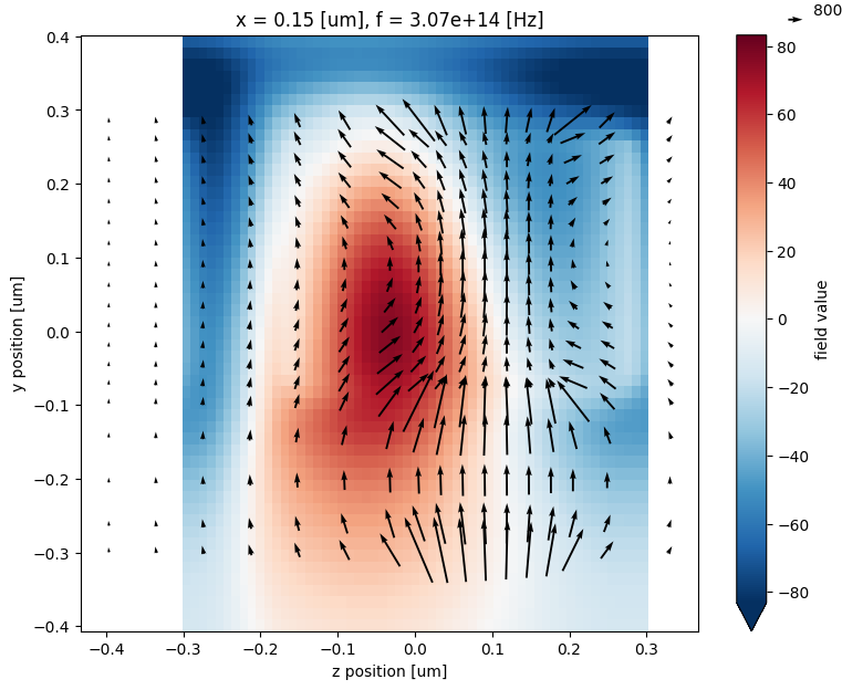
# average (or sum) over space first
spectrum = simData["y"].intensity.mean(dim=["y", "z"])  # adjust dims if needed

# find peak frequency index
idx = spectrum.argmax(dim="f")

# downsample the field data for more clear quiver plotting
sampling=3
field_ds_y_resampled = field_ds_y.sel(z=slice(None, None, sampling), y=slice(None, None, sampling))

f, ax = plt.subplots(figsize=(9, 7))
field_ds_y.isel(x=0).isel(f=idx).Ex.real.plot.imshow(x="y", y="z", ax=ax, robust=True)
field_ds_y_resampled.isel(x=0).isel(f=idx).real.plot.quiver("z", "y", "Ez", "Ey", ax=ax)
plt.savefig("quiver_yz_Ex.png")
plt.show()
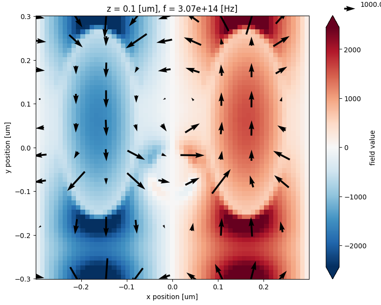
# average (or sum) over space first
spectrum = simData["z"].intensity.mean(dim=["x", "y"])  # adjust dims if needed

# find peak frequency index
idx = spectrum.argmax(dim="f")

# downsample the field data for more clear quiver plotting
field_ds_z_resampled = field_ds_z.sel(x=slice(None, None, 7), y=slice(None, None, 7))

f, ax = plt.subplots(figsize=(9, 7))
field_ds_z.isel(z=0).isel(f=idx).Ey.real.plot.imshow(x="x", y="y", ax=ax, robust=True)
field_ds_z_resampled.isel(z=0).isel(f=idx).real.plot.quiver("x", "y", "Ex", "Ey", ax=ax)
plt.show()
# average (or sum) over space first
spectrum = simData["y"].intensity.mean(dim=["z", "y"])  # adjust dims if needed

# find peak frequency index
idx = spectrum.argmax(dim="f")

# # get frequency value
f_peak = simData["y"].intensity.isel(f=idx)
f_peak_ref = simData_ref["y"].intensity.isel(f=idx)
f_peak_field = np.sqrt(f_peak)

# Divide out the scaling factor
alpha = np.sqrt(np.max(f_peak_ref)).values

# plot the peak
(f_peak_field / alpha).transpose("z", "y").plot(figsize=(6, 7), cmap="magma")
<matplotlib.collections.QuadMesh at 0x30fe7c3d0>
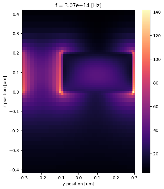
print(f"Field Enhancement: {np.max(f_peak_field / alpha).values}")
Field Enhancement: 141.87673950195312