





Author: Oliver Kuster, Karlsruhe Institute of Technology
One of the main challenges for photonic integrated circuits (PIC) is the efficient coupling of light from a fiber into the PIC. One common method uses grating couplers. While such grating couplers can reach notable coupling efficiencies (>80%), their basic planar geometry tends to be sensitive to the polarization of the incoming light. The optimization for both polarizations does tend to be challenging when using only 2D designs. By making use of full 3D Topology Optimization, highly efficient polarization-insensitive grating couplers can be designed.
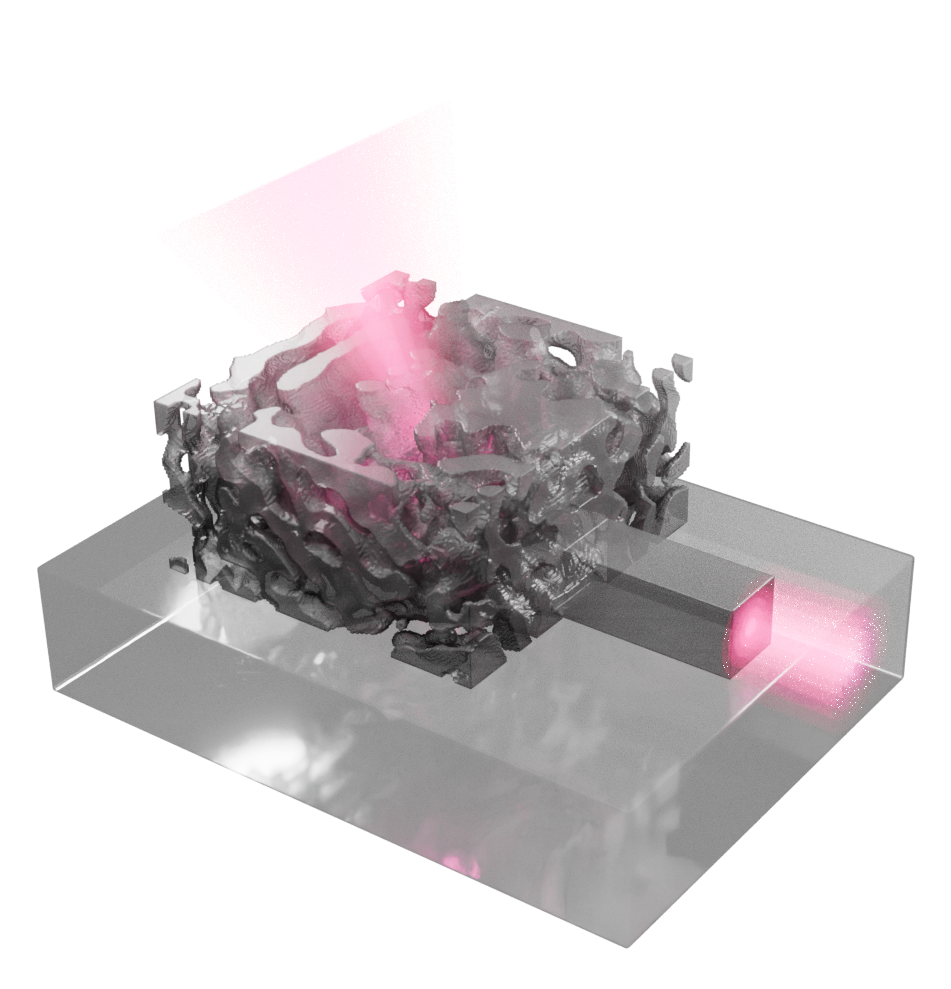
Here, we present the outline for the density-based topology optimization of a 3D polarization-insensitive grating coupler. This notebook is meant to serve as an example optimization for a smaller coupler. Since the full, large-scale optimization is too complex and too costly to put into a short notebook, we present a coupler with half the spatial footprint and an incoming beam at half the usual size. The full details of how the optimization is done on a full-scale coupler can be found in Kuster et al. The goal of this optimization is to build a coupler which can efficiently couple an incoming x-polarized wave into a waveguide, as well as an incoming y-polarized wave. By making use of the third dimension, additional complexity can be encoded by the additionally available degrees of freedom. An example of such a polarization-independent grating coupler can be seen in the image below. We will implement a smaller version of that grating coupler with a smaller feature size to obtain a performant polarization-independent grating coupler in a fast manner.
Reference: O. Kuster et al., IEEE J. Sel. Top. Quantum Electron. vol. 32, pp. 1-8 (2026) DOI:10.1109/JSTQE.2026.3657231
import numpy as np
import matplotlib.pyplot as plt
import matplotlib.colors as colors
import pyvista as pv

import tidy3d as td
import tidy3d.web as web

from tidy3d.plugins.autograd import (
    make_filter_and_project,
    rescale,
    adam,
    apply_updates,
)
import autograd.numpy as anp
from autograd import value_and_grad

np.random.seed(42)
Setting Up the Simulation
First we need to set up the parameters of our illumination source. We assume a Gaussian beam with a beam width of $5.2~$µm and a tilt of 10°. The grating coupler is optimized for a wavelength of $1.55~$µm, which we need to convert into a frequency for Tidy3D.
wavelength = 1.55
freq0 = td.C_0 / wavelength
fwidth = freq0 / 10
run_time = 50 / fwidth

fiber_tilt = 10
spot_size = 5.2
Next up we set up the simulation domain and its parameters. The setup consists of a fully 3D design region for the grating coupler and the outgoing waveguide. Both grating coupler and waveguide will have a permittivity of $1.53^2$, which is a typical refractive index for the polymers used for 3D laser-nanoprinting. The entire setup is then placed on top of a substrate made out of glass with a permittivity of $1.444^2$
rho_size = (10, 10, 5)
thickness_substrate = 4
buffer = 1 * wavelength
# dpml = 0.5

wg_width = 2
wg_height = 2
wg_length = 5

Lx = wg_length + rho_size[0]
Ly = wg_length + rho_size[1]
Lz = thickness_substrate + rho_size[2] + buffer

eps_design = 1.53**2
eps_substrate = 1.444**2
eps_air = 1
And finally also the parameters on how to discretize the simulation and the design region.
# dl = wavelength / 20
nx = 200
ny = 100
nz = 100

min_steps_per_wl = 10
Next we want to parametrize the structures in the simulation. To do so, we define a simple function which returns the substrate and the waveguide for us to put into the simulation for Tidy3D.
def simulation_structures():
    """
    Sets up the list of structures present in the simulation, which are not the design region.
    """

    def make_substrate():
        """
        Sets up the substrate.
        """
        substrate = td.Structure(
            geometry=td.Box.from_bounds(
                rmin=(-td.inf, -td.inf, -Lz / 2 - thickness_substrate),
                rmax=(td.inf, td.inf, -rho_size[2] / 2),
            ),
            medium=td.Medium(permittivity=eps_substrate),
        )
        return substrate

    def make_waveguide():
        """
        Sets up the output waveguide.
        """
        waveguide = td.Structure(
            geometry=td.Box(
                center=(Lx / 2, 0, -rho_size[2] / 2 + wg_width / 2),
                size=(wg_length, wg_width, wg_height),
            ),
            medium=td.Medium(permittivity=eps_design),
        )
        return waveguide

    return [make_substrate(), make_waveguide()]


def make_design_region(rho, beta, rmin):
    """
    Generates the design region for the simulation. The input density rho is converted into the permittivity eps by filtering, projection and linear interpolation.
    Note that we use symmetry so we only need to initialize half the design region.
    rho:        Input density for the topology optimization.
    beta:       Degree of binarization for the projection.
    rmin:       Minimum feature size for the filtering.
    Returns:    Design region.
    """
    filt_proj = make_filter_and_project(rmin, dl=rho_size[0] / nx)
    rho_pre = filt_proj(rho, beta)
    eps = rescale(rho_pre, eps_air, eps_design)

    dr_center_y = rho_size[1] / 4
    dr_size_y = rho_size[1] / 2

    geometry = td.Box(
        center=(0, dr_center_y, 0), size=(rho_size[0], dr_size_y, rho_size[2])
    )

    custom_structure = td.Structure.from_permittivity_array(
        geometry=geometry, eps_data=eps
    )

    return [custom_structure]
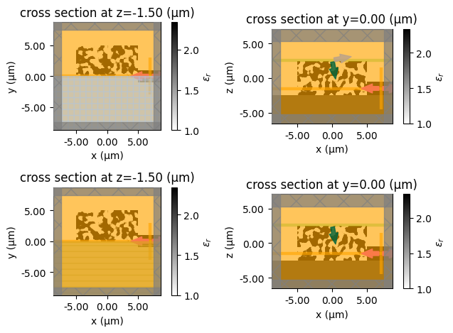
Now that we have the substrate, waveguide and design region, we can put them all together into a simulation. Since we are interested in a polarization independent coupler, we need two simulations. One for x-polarized light and one for y-polarized light. We also make use of the symmetry to not only reduce the computational domain but also differentiate between the polarizations and waveguide modes which we want to couple.
So first, we set up the sources.
src_pos = rho_size[2] / 2 + 0.1
mon_pos_x = rho_size[0] / 2 + 2
mon_pos_z = -rho_size[2] / 2 + wg_height / 2

mode_spec = td.ModeSpec(num_modes=1, target_neff=eps_design)

# For monitoring and plotting
wavelengths = np.linspace(wavelength - 0.05, wavelength + 0.05, 21)
freqs = td.C_0 / wavelengths
And then also the monitors.
# For evaluating the loss/figure of merit
fom_monitor = td.ModeMonitor(
    center=[mon_pos_x, 0, mon_pos_z],
    size=[0, 3 * wg_width, 3 * wg_width],
    freqs=freq0,
    mode_spec=mode_spec,
    name="fom_monitor",
)

# Monitors for visualizing the results. The coordinates indicate in which plane they lie.
mode_monitor = td.ModeMonitor(
    center=[mon_pos_x, 0, mon_pos_z],
    size=[0, 3 * wg_width, 3 * wg_width],
    freqs=freqs,
    mode_spec=mode_spec,
    name="mode_monitor",
)


field_monitor_y = td.FieldMonitor(
    center=(0, 0, 0), size=(td.inf, 0, td.inf), freqs=[freq0], name="FieldMonitor_y"
)

field_monitor_z = td.FieldMonitor(
    center=(0, 0, -rho_size[2] / 2 + wg_width / 2),
    size=(td.inf, td.inf, 0),
    freqs=[freq0],
    name="FieldMonitor_z",
)

eps_monitor_y = td.PermittivityMonitor(
    center=(0, 0, 0),
    size=(td.inf, 0, td.inf),
    freqs=[freq0],
    name="PermittivityMonitor_y",
)

eps_monitor_z = td.PermittivityMonitor(
    center=(0, 0, -rho_size[2] / 2 + wg_width / 2),
    size=(td.inf, td.inf, 0),
    freqs=[freq0],
    name="PermittivityMonitor_z",
)

source_xpol = td.GaussianBeam(
    center=(0, 0, src_pos),
    size=(td.inf, td.inf, 0),
    source_time=td.GaussianPulse(freq0=freq0, fwidth=fwidth),
    pol_angle=0,  # Polarization is set here.
    angle_theta=-fiber_tilt * np.pi / 180.0,
    direction="-",
    num_freqs=1,
    waist_radius=spot_size / 2,
)

source_ypol = td.GaussianBeam(
    center=(0, 0, src_pos),
    size=(td.inf, td.inf, 0),
    source_time=td.GaussianPulse(freq0=freq0, fwidth=fwidth),
    pol_angle=np.pi / 2,  # Polarization is set here.
    angle_theta=-fiber_tilt * np.pi / 180.0,
    direction="-",
    num_freqs=1,
    waist_radius=spot_size / 2,
)


def make_sim(rho, beta=1.0, rmin=0.01):
    """
    Generates the simulation object.
    rho:        Input density for the topology optimization.
    beta:       Degree of binarization for the projection.
    rmin:       Minimum feature size for the filtering.
    Returns:    Pair of tidy3d simulation objects, for x- and y-polarized light respectively.
    """
    eps = make_design_region(rho, beta, rmin)
    structures = simulation_structures()

    em_sim_xpol = td.Simulation(
        size=(Lx, Ly, Lz),
        run_time=run_time,
        structures=structures + eps,
        sources=[source_xpol],
        monitors=[
            fom_monitor,
            mode_monitor,
            field_monitor_y,
            field_monitor_z,
            eps_monitor_y,
            eps_monitor_z,
        ],
        grid_spec=td.GridSpec.auto(
            min_steps_per_wvl=min_steps_per_wl, wavelength=wavelength
        ),
        boundary_spec=td.BoundarySpec(
            x=td.Boundary.pml(), y=td.Boundary.pml(), z=td.Boundary.pml()
        ),
        symmetry=(0, 1, 0),  # To simulate the coupling into the TE00 mode.
    )

    em_sim_ypol = td.Simulation(
        size=(Lx, Ly, Lz),
        run_time=run_time,
        structures=structures + eps,
        sources=[source_ypol],
        monitors=[
            fom_monitor,
            mode_monitor,
            field_monitor_y,
            field_monitor_z,
            eps_monitor_y,
            eps_monitor_z,
        ],
        grid_spec=td.GridSpec.auto(
            min_steps_per_wvl=min_steps_per_wl, wavelength=wavelength
        ),
        boundary_spec=td.BoundarySpec(
            x=td.Boundary.pml(), y=td.Boundary.pml(), z=td.Boundary.pml()
        ),
        symmetry=(0, -1, 0),  # To simulate the coupling into the TM00 mode.
    )

    return em_sim_xpol, em_sim_ypol
Now let's see if we set up everything correctly by checking out some cross sections.
rho_0 = np.random.rand(nx, ny, nz)
beta_0 = 1e3
rmin_0 = 0.5

sim = make_sim(rho_0, beta_0, rmin_0)

fig, axs = plt.subplots(2, 2)
sim[0].plot_eps(z=-rho_size[2] / 2 + wg_width / 2, ax=axs[0, 0])
sim[1].plot_eps(z=-rho_size[2] / 2 + wg_width / 2, ax=axs[1, 0])
sim[0].plot_eps(y=0, ax=axs[0, 1])
sim[1].plot_eps(y=0, ax=axs[1, 1])
plt.tight_layout()
We can now also do a test run to see if everything runs through.
sim_results = web.run(sim[0], "test_run_gc_xpol", verbose=False)
Optimization
Now that we have the simulation set up, we can start with setting up the optimization. First, we need to define an objective function. The most simple form of an objective function which captures our design goal is simply maximizing the average of the coupling efficiencies of each polarization into their respective waveguide modes.
$$L(\rho(\mathbf{r})) = \frac{\text{CE}_\text{TE00} + \text{CE}_\text{TM00}}{2}$$
def measure_avg_ce(sim_data):
    """
    Function to obtain the average coupling efficiency out of the two simulations which were put in by sim_data.
    sim_data:   Pair of the simulation data, x- and y-polarized light respectively.
    returns:    Average coupling efficiency of the two input simulations.
    """
    output_amps_xpol = sim_data[0]["fom_monitor"].amps
    amp_xpol = output_amps_xpol.sel(direction="+", f=freq0, mode_index=0).values

    output_amps_ypol = sim_data[1]["fom_monitor"].amps
    amp_ypol = output_amps_ypol.sel(direction="+", f=freq0, mode_index=0).values

    return (anp.sum(anp.abs(amp_xpol) ** 2) + anp.sum(anp.abs(amp_ypol) ** 2)) / 2


def objective_fn(rho, step_num, beta=1, rmin=0.01):
    """
    Wraps the actual objective function for "bookkeeping".
    rho:        Input density for the topology optimization.
    step_num:   Current iteration of the optimization.
    beta:       Degree of binarization for the projection.
    rmin:       Minimum feature size for the filtering.
    returns:    Average coupling efficiency of x-pol->TE00 and y-pol->TM00 given the input density rho.
    """
    sim = make_sim(rho, beta, rmin)

    task_name_x = "grating_coupler_xpol"
    task_name_y = "grating_coupler_ypol"
    task_name_x += f"_step_{step_num}"
    task_name_y += f"_step_{step_num}"
    sim_data_xpol = web.run(
        sim[0], task_name=task_name_x, folder_name="grating_coupler_pol", verbose=False
    )
    sim_data_ypol = web.run(
        sim[1], task_name=task_name_y, folder_name="grating_coupler_pol", verbose=False
    )

    sim_data_xpol.to_file("sim_data_xpol.hdf5")
    sim_data_ypol.to_file("sim_data_ypol.hdf5")

    return measure_avg_ce([sim_data_xpol, sim_data_ypol])
Let's test if everything works by calculating the value and gradients of the objective function and then also plotting the gradients.
dL_drho = value_and_grad(objective_fn)

val, grad = dL_drho(rho_0, 0, beta_0, rmin_0)

filt_proj = make_filter_and_project(rmin_0, dl=rho_size[0] / nx)
rho_0_pre = filt_proj(rho_0, beta_0)

fig, axs = plt.subplots(1, 2, sharey=True)
axs[0].imshow(
    rho_0_pre[:, :, rho_0_pre.shape[2] // 2].T,
    origin="lower",
    cmap="binary",
    extent=(0, rho_size[0], 0, rho_size[1] / 2),
)
axs[0].set_xlabel(r"$x~$($\mathregular{\mu}$m)")
axs[0].set_ylabel(r"$y~$($\mathregular{\mu}$m)")
axs[0].set_title(r"$\rho$")
axs[1].imshow(
    grad[:, :, grad.shape[2] // 2].T,
    origin="lower",
    cmap="magma",
    extent=(0, rho_size[0], 0, rho_size[1] / 2),
)
axs[1].set_xlabel(r"$x~$($\mathregular{\mu}$m)")
axs[1].set_title(r"dL/d$\rho$");
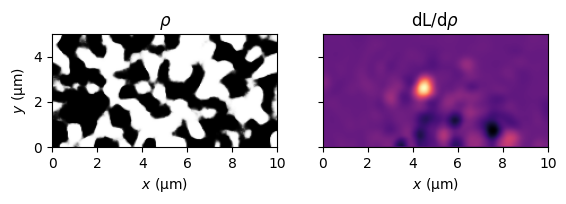
We set up a small-scale optimization. Since we are working with density based topology optimization, we want to start off with a low binarization level $\beta$ and start to increase $\beta$ during the optimization to improve convergence. Using the Adam-optimizer, we are able to find an efficient and functioning design, which makes use of all three spatial dimensions to reach a rather high coupling efficiency for both polarizations.
num_steps = 20
learning_rate = 0.5

rho_0 = np.random.rand(nx, ny, nz)
beta = beta_0 = 1
beta_increment = 1
rmin_0 = 0.4
loss_hist = []

optimizer = adam(learning_rate=learning_rate)
opt_state = optimizer.init(rho_0)

filt_proj = make_filter_and_project(rmin_0, dl=rho_size[0] / nx)


def extra_information(sim_data):
    """
    Function to track and visualize the results for the notebook.
    sim_data:   Pair of input simulations
    """

    permittivity_xy = np.real(
        sim_data[0]["PermittivityMonitor_z"].eps_xx.values
    ).squeeze()
    permittivity_xz = np.real(
        sim_data[1]["PermittivityMonitor_y"].eps_xx.values
    ).squeeze()

    field_xpol_xy = np.sqrt(
        np.abs(sim_data[0]["FieldMonitor_z"].Ex.values) ** 2
        + np.abs(sim_data[0]["FieldMonitor_z"].Ey.values) ** 2
        + np.abs(sim_data[0]["FieldMonitor_z"].Ez.values) ** 2
    ).squeeze()
    field_xpol_xz = np.sqrt(
        np.abs(sim_data[0]["FieldMonitor_y"].Ex.values) ** 2
        + np.abs(sim_data[0]["FieldMonitor_y"].Ey.values) ** 2
        + np.abs(sim_data[0]["FieldMonitor_y"].Ez.values) ** 2
    ).squeeze()

    field_ypol_xy = np.sqrt(
        np.abs(sim_data[1]["FieldMonitor_z"].Ex.values) ** 2
        + np.abs(sim_data[1]["FieldMonitor_z"].Ey.values) ** 2
        + np.abs(sim_data[1]["FieldMonitor_z"].Ez.values) ** 2
    ).squeeze()
    field_ypol_xz = np.sqrt(
        np.abs(sim_data[1]["FieldMonitor_y"].Ex.values) ** 2
        + np.abs(sim_data[1]["FieldMonitor_y"].Ey.values) ** 2
        + np.abs(sim_data[1]["FieldMonitor_y"].Ez.values) ** 2
    ).squeeze()

    output_amps_xpol = sim_data[0]["mode_monitor"].amps
    amp_xpol = np.abs(output_amps_xpol.sel(direction="+", mode_index=0).values) ** 2
    output_amps_ypol = sim_data[1]["mode_monitor"].amps
    amp_ypol = np.abs(output_amps_ypol.sel(direction="+", mode_index=0).values) ** 2

    return (
        (permittivity_xy, permittivity_xz),
        (field_xpol_xy, field_xpol_xz),
        (field_ypol_xy, field_ypol_xz),
        (amp_xpol, amp_ypol),
    )
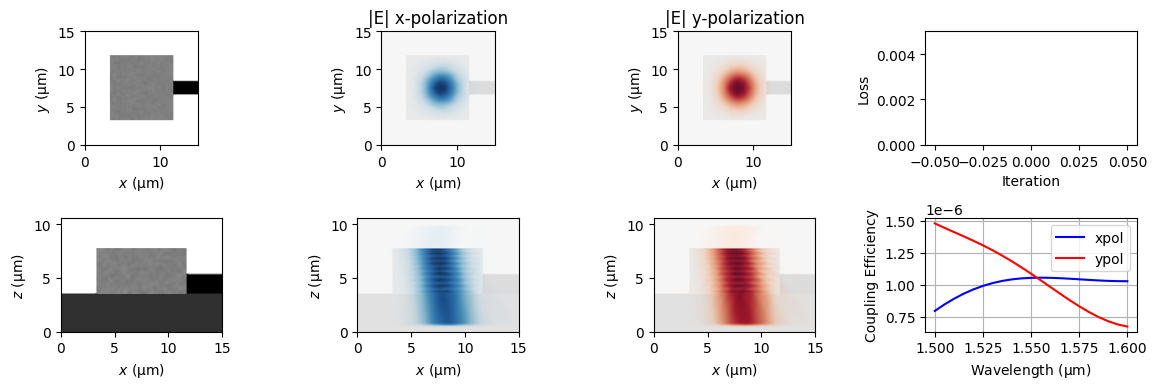
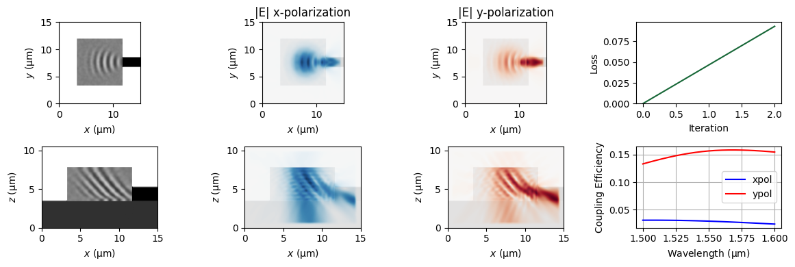
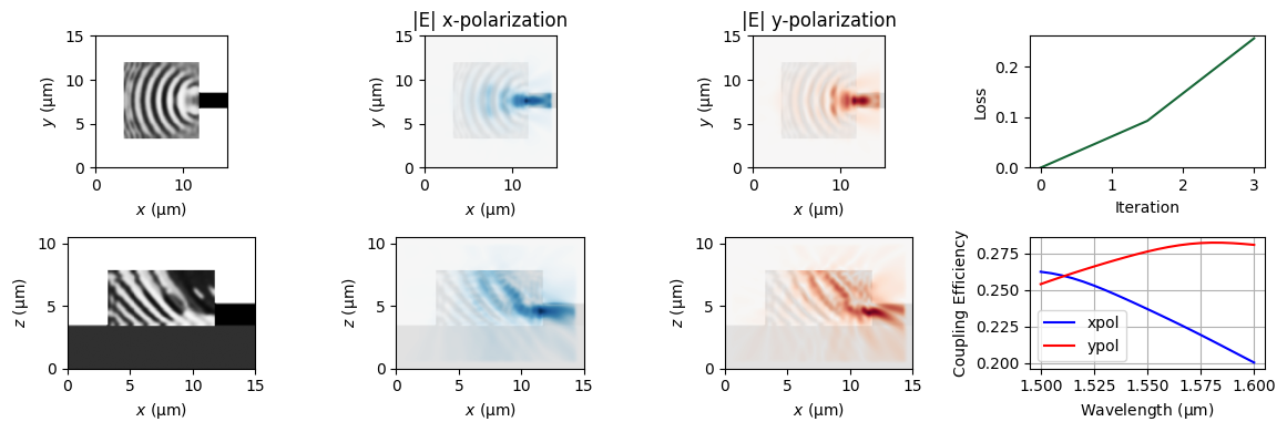
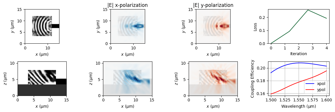
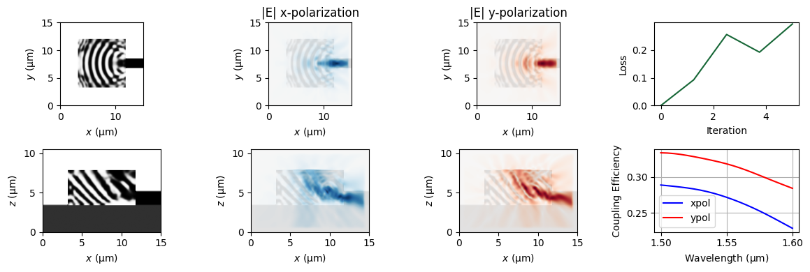
Now we are ready to run the optimization. To track the progress of the optimization we also plot the cross sections of our design as well as the absolute value of the electric fields for each polarization. Additionally, we also track the loss as well as the coupling efficiency to see how the optimization performs.
for i in range(num_steps):
    rho_filt_proj = filt_proj(rho_0, beta)

    beta = beta_0 + i * beta_increment
    value, grad = value_and_grad(objective_fn)(rho_0, i, beta, rmin_0)

    sim_xpol = td.SimulationData.from_file(fname="sim_data_xpol.hdf5")
    sim_ypol = td.SimulationData.from_file(fname="sim_data_ypol.hdf5")

    permittivity, field_xpol, field_ypol, ce = extra_information([sim_xpol, sim_ypol])

    loss_hist.append(value)

    fig, axs = plt.subplots(2, 4, figsize=(12, 4))
    # Plot the permittivities.
    axs[0, 0].imshow(
        permittivity[0].T, origin="lower", cmap="binary", extent=(0, Lx, 0, Ly)
    )
    axs[0, 0].set_xlabel(r"$x~$($\mathregular{\mu}$m)")
    axs[0, 0].set_ylabel(r"$y~$($\mathregular{\mu}$m)")
    axs[1, 0].imshow(
        permittivity[1].T, origin="lower", cmap="binary", extent=(0, Lx, 0, Lz)
    )
    axs[1, 0].set_xlabel(r"$x~$($\mathregular{\mu}$m)")
    axs[1, 0].set_ylabel(r"$z~$($\mathregular{\mu}$m)")

    # Plot the field for the x-polarization.
    axs[0, 1].imshow(
        permittivity[0].T, origin="lower", cmap="binary", extent=(0, Lx, 0, Ly)
    )
    axs[0, 1].imshow(
        field_xpol[0].T,
        origin="lower",
        cmap="RdBu",
        extent=(0, Lx, 0, Ly),
        alpha=0.9,
        norm=colors.CenteredNorm(),
    )
    axs[0, 1].set_xlabel(r"$x~$($\mathregular{\mu}$m)")
    axs[0, 1].set_ylabel(r"$y~$($\mathregular{\mu}$m)")
    axs[0, 1].set_title("|E| x-polarization")
    axs[1, 1].imshow(
        permittivity[1].T, origin="lower", cmap="binary", extent=(0, Lx, 0, Lz)
    )
    axs[1, 1].imshow(
        field_xpol[1].T,
        origin="lower",
        cmap="RdBu",
        extent=(0, Lx, 0, Lz),
        alpha=0.9,
        norm=colors.CenteredNorm(),
    )
    axs[1, 1].set_xlabel(r"$x~$($\mathregular{\mu}$m)")
    axs[1, 1].set_ylabel(r"$z~$($\mathregular{\mu}$m)")

    # Plot the field for the y-polarization.
    axs[0, 2].imshow(
        permittivity[0].T, origin="lower", cmap="binary", extent=(0, Lx, 0, Ly)
    )
    axs[0, 2].imshow(
        field_ypol[0].T,
        origin="lower",
        cmap="RdBu_r",
        extent=(0, Lx, 0, Ly),
        alpha=0.9,
        norm=colors.CenteredNorm(),
    )
    axs[0, 2].set_xlabel(r"$x~$($\mathregular{\mu}$m)")
    axs[0, 2].set_ylabel(r"$y~$($\mathregular{\mu}$m)")
    axs[0, 2].set_title("|E| y-polarization")
    axs[1, 2].imshow(
        permittivity[1].T, origin="lower", cmap="binary", extent=(0, Lx, 0, Lz)
    )
    axs[1, 2].imshow(
        field_ypol[1].T,
        origin="lower",
        cmap="RdBu_r",
        extent=(0, Lx, 0, Lz),
        alpha=0.9,
        norm=colors.CenteredNorm(),
    )
    axs[1, 2].set_xlabel(r"$x~$($\mathregular{\mu}$m)")
    axs[1, 2].set_ylabel(r"$z~$($\mathregular{\mu}$m)")

    # Plot of the loss.
    axs[0, 3].plot(np.linspace(0, i + 1, i + 1), loss_hist)
    axs[0, 3].set_ylim(0, np.max(loss_hist) + 0.005)
    axs[0, 3].set_xlabel("Iteration")
    axs[0, 3].set_ylabel("Loss")

    # Plot of the coupling efficiencies.
    axs[1, 3].plot(wavelengths, ce[0], color="blue", label="xpol")
    axs[1, 3].plot(wavelengths, ce[1], color="red", label="ypol")
    axs[1, 3].set_xlabel(r"Wavelength$~$($\mathregular{\mu}$m)")
    axs[1, 3].set_ylabel("Coupling Efficiency")
    axs[1, 3].legend()
    axs[1, 3].grid()

    plt.tight_layout()
    plt.show()

    print(f"step = {i + 1}")
    print(f"\tbeta = {beta:.4e}")
    print(f"\tloss = {value:.4e}")
    print(f"\tgrad_norm = {np.linalg.norm(grad):.4e}")

    updates, opt_state = optimizer.update(-grad, opt_state, rho_0)
    rho_0[:] = apply_updates(rho_0, updates)

    anp.clip(rho_0, 0.0, 1.0, out=rho_0)
step = 1
	beta = 1.0000e+00
	loss = 1.0694e-06
	grad_norm = 3.7599e-06
step = 2
	beta = 2.0000e+00
	loss = 9.3022e-02
	grad_norm = 2.3585e-03
step = 3
	beta = 3.0000e+00
	loss = 2.5675e-01
	grad_norm = 3.7196e-03
step = 4
	beta = 4.0000e+00
	loss = 1.9284e-01
	grad_norm = 4.2128e-03
step = 5
	beta = 5.0000e+00
	loss = 2.9483e-01
	grad_norm = 3.9010e-03
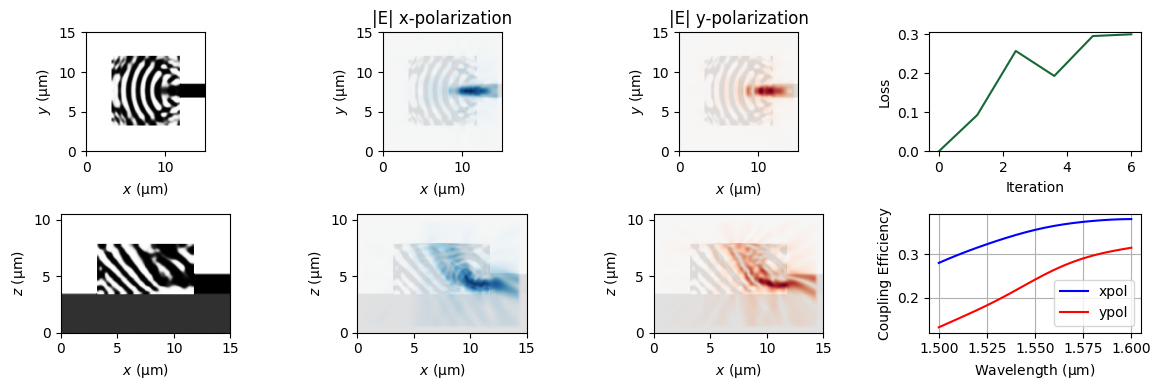
step = 6
	beta = 6.0000e+00
	loss = 2.9932e-01
	grad_norm = 6.7845e-03
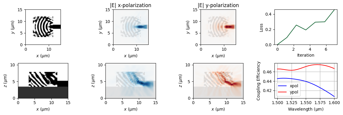
step = 7
	beta = 7.0000e+00
	loss = 4.5521e-01
	grad_norm = 4.2894e-03
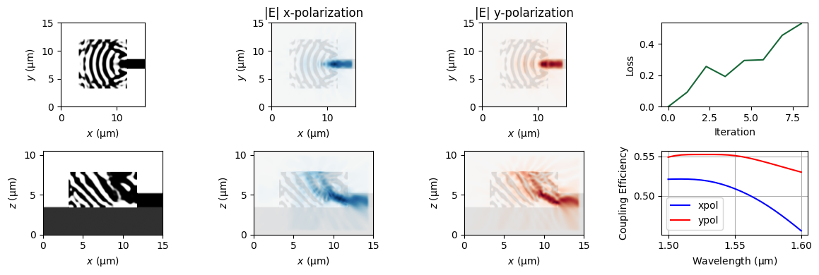
step = 8
	beta = 8.0000e+00
	loss = 5.2996e-01
	grad_norm = 4.9093e-03
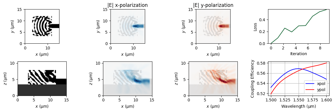
step = 9
	beta = 9.0000e+00
	loss = 5.6676e-01
	grad_norm = 5.1746e-03
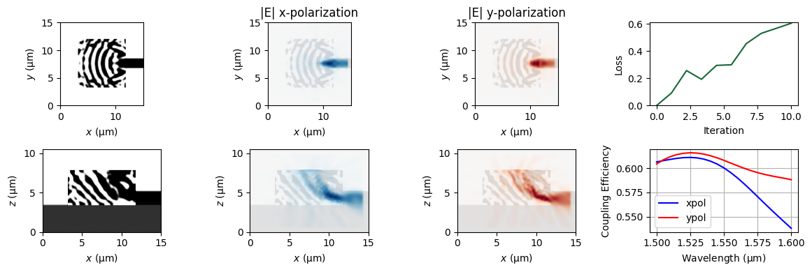
step = 10
	beta = 1.0000e+01
	loss = 6.0413e-01
	grad_norm = 3.8927e-03
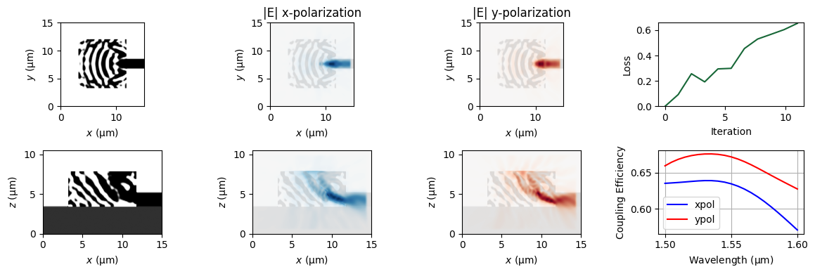
step = 11
	beta = 1.1000e+01
	loss = 6.5344e-01
	grad_norm = 2.1332e-03
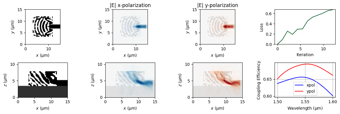
step = 12
	beta = 1.2000e+01
	loss = 6.7502e-01
	grad_norm = 2.4291e-03
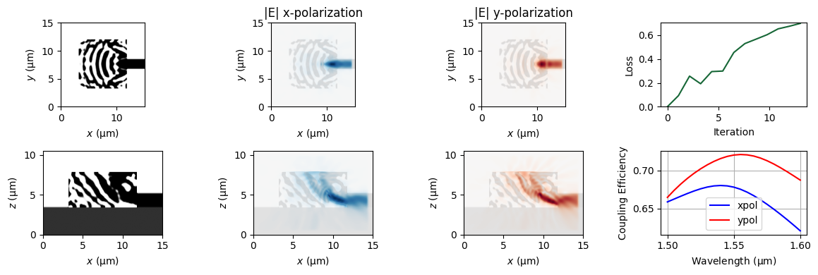
step = 13
	beta = 1.3000e+01
	loss = 6.9931e-01
	grad_norm = 1.9025e-03
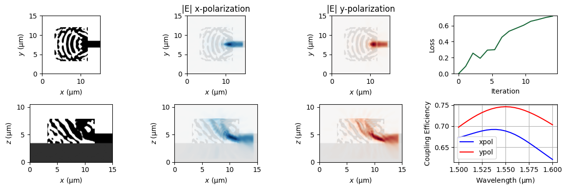
step = 14
	beta = 1.4000e+01
	loss = 7.1737e-01
	grad_norm = 1.6485e-03
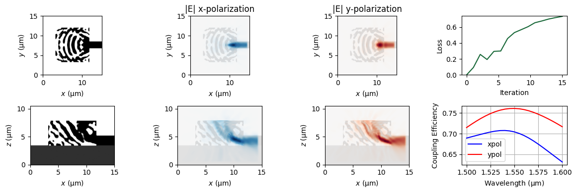
step = 15
	beta = 1.5000e+01
	loss = 7.3265e-01
	grad_norm = 1.9050e-03
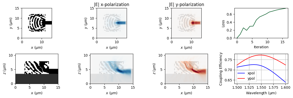
step = 16
	beta = 1.6000e+01
	loss = 7.4631e-01
	grad_norm = 1.3152e-03
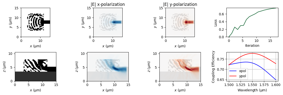
step = 17
	beta = 1.7000e+01
	loss = 7.5415e-01
	grad_norm = 1.4350e-03
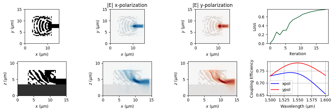
step = 18
	beta = 1.8000e+01
	loss = 7.6111e-01
	grad_norm = 1.6857e-03
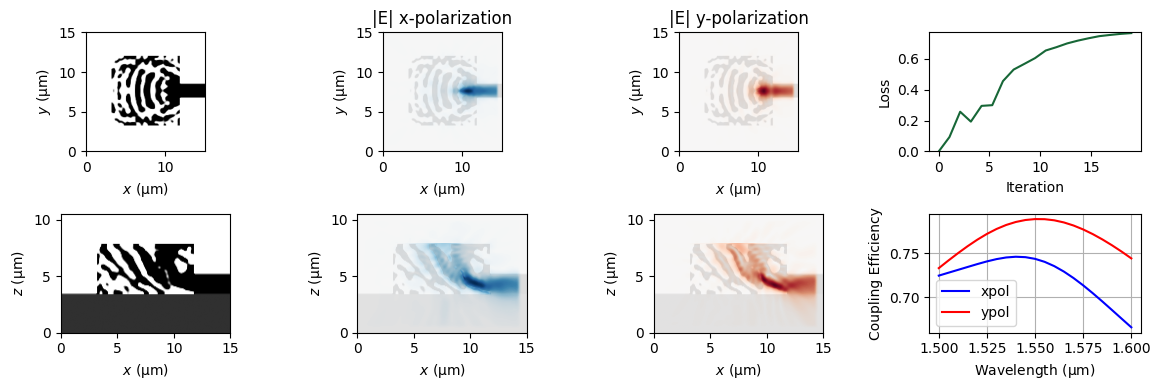
step = 19
	beta = 1.9000e+01
	loss = 7.6615e-01
	grad_norm = 3.1045e-03
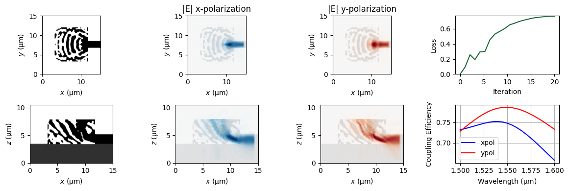
step = 20
	beta = 2.0000e+01
	loss = 7.6689e-01
	grad_norm = 3.7429e-03
Last, but not least, we also want to plot the final design.
sim_opt = make_sim(rho_0, beta, rmin_0)
eps = np.real(
    sim_opt[0].epsilon(
        td.Box(
            center=(0, 0, 0),
            size=(Lx, Ly, Lz),
        )
    )
)

p = pv.Plotter(off_screen=True)
data = pv.wrap(eps.values)
p.add_mesh(data.contour(), cmap="binary")
p.camera_position = "yz"
p.camera.elevation = 30
p.camera.azimuth = 30
p.remove_scalar_bar()
p.show(jupyter_backend="static")
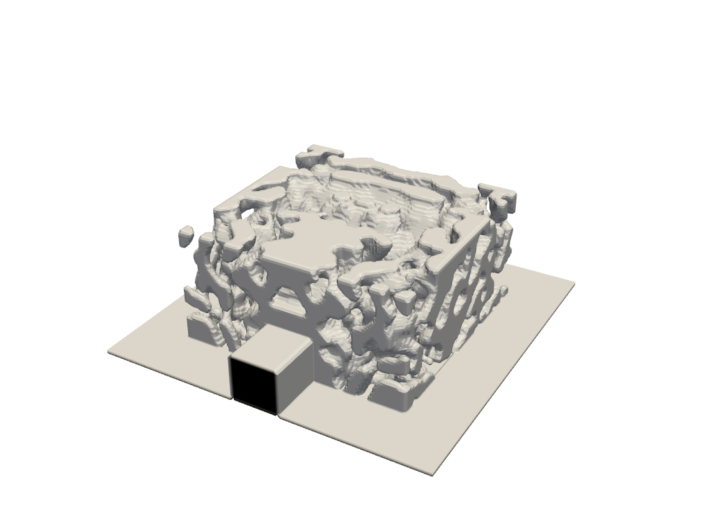
We see that we are able to reach a coupling efficiency of over 75% for both polarizations. We want to note that this however is not a realistically fabricable structure. Not only is the feature size smaller than what would be realistically fabricable, we also do not consider the structural integrity of the device. These are aspects which will decrease the overall coupling efficiency of the device, however improving upon the optimization itself can mitigate said decrease in coupling efficiency. These results here are meant to show how in principle such a coupler can be implemented in a lightweight and cheap manner. A full-scale optimization of course would take much longer and be more costly.


 TERMS & CONDITIONS


 How the process works:
 Try this real URL to see an example: