This notebook demonstrates a two-stage inverse design workflow for building a higher-order mode launcher in a dielectric slab waveguide. The goal is to couple the fundamental mode (TE0) of a narrow waveguide into the TE2 mode of a wider output waveguide.
The device is split into two cascaded components, each optimized independently before being combined into a single verification simulation:
- Mode converter — a compact pixelated design region that converts TE0 to TE2 within a waveguide of constant width. It is parameterized as a continuous permittivity field and solved with topology optimization, using a filter/project scheme and an erosion/dilation penalty to enforce a minimum feature size.
- Linear taper — a symmetric polygonal taper that expands the waveguide width while preserving the TE2 content. It is parameterized by the half-width at a few control points and optimized with a curvature penalty to discourage sharp bends.
Both stages use tidy3d's autograd integration to compute gradients of the objective through the FDTD simulation.

import tidy3d as td
import tidy3d.web as web
import numpy as np
import matplotlib.pyplot as plt
import autograd.numpy as anp
import autograd as ag
import optax
from tidy3d.plugins.autograd import make_filter_and_project, rescale, make_erosion_dilation_penalty, value_and_grad, make_curvature_penalty
from tidy3d.plugins.mode import ModeSolver
from tidy3d.plugins.mode.web import run as run_mode_solver
09:32:08 -03 WARNING: Using canonical configuration directory at
             '/home/filipe/.config/tidy3d'. Found legacy directory at
             '~/.tidy3d', which will be ignored. Remove it manually or run
             'tidy3d config migrate --delete-legacy' to clean up.
Setup
Define the central wavelength, the waveguide material, the geometry of the two devices, and the resolution of the design grid used by the topology optimization.
# 1. GENERAL SETUP

print(" Step 1: General Setup ")

wavelength = 1.0
freq0 = td.C_0 / wavelength

# Materials
eps_wg = 2.75
wg_medium = td.Medium(permittivity=eps_wg)

# Dimensions
lx_conv = 5.0  # Converter Length
ly_conv = 3.0  # Converter Width
wg_width_conv = 1.2
output_wg_length = 3.0

# Grid & Design Resolution
dl_design = 0.01
nx = int(lx_conv / dl_design)
ny = int(ly_conv / dl_design)

# Initial Random Parameters
# Seed the RNG so the optimization starts from a reproducible initial density.
np.random.seed(0)
params0_conv = np.random.random((nx, ny))

print(f"Setup Complete. Wavelength: {wavelength} um")
 Step 1: General Setup
Setup Complete. Wavelength: 1.0 um
Input Waveguide Mode Analysis
Before setting up the optimization, run a quick mode solver on the input waveguide to confirm that the desired mode indices exist and to inspect the field profiles of the lowest-order modes.
# STEP 1.5: MODE ANALYSIS

print(" Step 1.5: Running Mode Analysis ")

wg_input_analysis = td.Structure(
    geometry=td.Box(center=(-lx_conv, 0, 0), size=(lx_conv, wg_width_conv, td.inf)), # center = (-5.0, 0, 0), size = (5.0, 1.2, inf)
    medium=wg_medium
)

mode_size = (0, wg_width_conv * 4, td.inf) # size = (0, 4.8, inf)
source_x_pos = -lx_conv # -5.0

plane = td.Box(center=[source_x_pos, 0, 0], size=mode_size) # size = (0, 4.8, inf)

sim_mode = td.Simulation(
    size=(1, ly_conv + 2, 0), # size = (1, 5.0, 0)
    center=(source_x_pos, 0, 0), # center = (-5.0, 0, 0)
    grid_spec=td.GridSpec.auto(min_steps_per_wvl=20, wavelength=wavelength), # min_steps_per_wvl=20
    structures=[wg_input_analysis],
    run_time=1e-12,
    boundary_spec=td.BoundarySpec.pml(x=False, y=True, z=False),
    sources=[],
    monitors=[]
)

num_modes = 4
mode_spec_analysis = td.ModeSpec(num_modes=num_modes)

mode_solver = ModeSolver(
    simulation=sim_mode,
    plane=plane,
    mode_spec=mode_spec_analysis,
    freqs=[freq0],
)

print("Running Advanced Mode Analysis on Server...")
modes = run_mode_solver(mode_solver, reduce_simulation=True, verbose=True)
 Step 1.5: Running Mode Analysis
Running Advanced Mode Analysis on Server...
09:32:13 -03 Mode solver created with
             task_id='fdve-17f5c92b-f588-44fa-b679-c413fc1bbe7e',
             solver_id='mo-db7cf02a-d2d8-4c59-91e3-578db2c975f6'.
Output()
Output()
09:32:17 -03 Mode solver status: success
Output()
print("Plotting Fields...")
fig, axs = plt.subplots(num_modes, 3, figsize=(12, 3 * num_modes), tight_layout=True)
for mode_index in range(num_modes):
    vmax = 1.1 * max(abs(modes.field_components[n].sel(mode_index=mode_index)).max() for n in ("Ex", "Ey", "Ez"))
    for field_name, ax in zip(("Ex", "Ey", "Ez"), axs[mode_index]):
        field = modes.field_components[field_name].sel(mode_index=mode_index)
        field.real.plot(label="Real", ax=ax)
        field.imag.plot(ls="--", label="Imag", ax=ax)
        ax.set_title(f"Mode {mode_index}, Field = {field_name}")
        ax.set_ylim(-vmax, vmax)
        ax.grid(True, alpha=0.3)
axs[0, 0].legend()
plt.show()
print("Effective indices: ", np.array(modes.n_eff))
Plotting Fields...
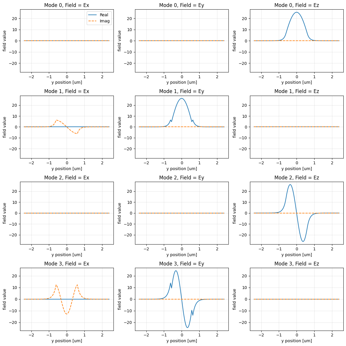
Effective indices: [[1.62160698 1.61255481 1.50846215 1.47129595]]
Part A: Topology Optimization Of The Mode Converter
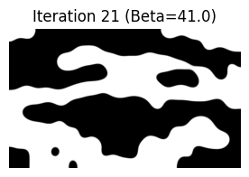
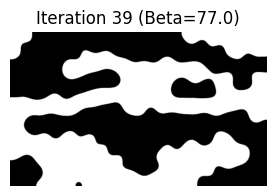
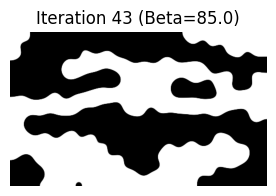
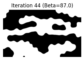
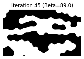
The converter is represented as a pixel grid of continuous density values between 0 and 1. A conic filter and a projection function (both provided by make_filter_and_project) smooth and binarize the density; the filtered values are then rescaled to a permittivity between air and the waveguide material. The projection sharpness is controlled by the parameter beta, which is annealed from soft to hard across iterations.
# PART A: MODE CONVERTER OPTIMIZATION

print(" PART A: MODE CONVERTER OPTIMIZATION ")

radius = 0.2
filter_project = make_filter_and_project(radius, dl_design)

def get_eps(params, beta):
    processed_params = filter_project(params, beta)
    eps = rescale(processed_params, 1, eps_wg)
    return eps
PART A: MODE CONVERTER OPTIMIZATION
Next, build the converter simulation as a function of the current parameters. The design region is a Structure.from_permittivity_array cell, sandwiched between input and output straight waveguides. A ModeSource launches the fundamental mode at the input and a ModeMonitor on the output measures the modal amplitudes.
def make_converter_sim(params, beta):
    eps_data = get_eps(params, beta).reshape((nx, ny, 1))
    converter_geo = td.Box(center=(0, 0, 0), size=(lx_conv, ly_conv, td.inf))
    converter_struct = td.Structure.from_permittivity_array(geometry=converter_geo, eps_data=eps_data)

    wg_input_struct = td.Structure(geometry=td.Box(center=(-lx_conv, 0, 0), size=(lx_conv, wg_width_conv, td.inf)),
                                   medium=wg_medium)
    wg_output_struct = td.Structure(geometry=td.Box(center=(lx_conv / 2 + output_wg_length / 2, 0, 0),
                                                    size=(output_wg_length, wg_width_conv, td.inf)), medium=wg_medium)

    mode_spec = td.ModeSpec(num_modes=4)
    forward_source = td.ModeSource(center=[-lx_conv / 2 - 0.5, 0, 0], size=(0, ly_conv + 2, td.inf),
                                   source_time=td.GaussianPulse(freq0=freq0, fwidth=freq0 / 10), direction='+',
                                   mode_index=0, mode_spec=mode_spec)
    measurement_monitor = td.ModeMonitor(center=[lx_conv / 2 + 1.0, 0, 0], size=(0, ly_conv + 2, td.inf), freqs=[freq0],
                                         mode_spec=mode_spec, name="measurement")

    return td.Simulation(size=(lx_conv + output_wg_length + 2, ly_conv + 2, 0),
                         grid_spec=td.GridSpec.auto(min_steps_per_wvl=25, wavelength=wavelength),
                         structures=[wg_input_struct, converter_struct, wg_output_struct], sources=[forward_source],
                         monitors=[measurement_monitor], run_time= 100 / (freq0 / 10),
                         boundary_spec=td.BoundarySpec.pml(x=True, y=True, z=False))
The figure of merit is the power coupled into the target output mode (TE2, mode_index=2). To promote binary solutions with manufacturable features, an erosion/dilation penalty is subtracted from the transmission, weighted by a factor that grows with beta.
mode_index_out = 2
penalty_fn = make_erosion_dilation_penalty(radius, dl_design)

def measure_power_conv(sim_data):
    amp = sim_data["measurement"].amps.sel(direction="+", f=freq0, mode_index=mode_index_out).values
    return anp.sum(anp.abs(amp) ** 2)

def J_conv(params, beta, step_num=None, verbose=False):
    sim = make_converter_sim(params, beta)
    sim_data = web.run(sim, task_name="opt_conv" + (f"_{step_num}" if step_num else ""), verbose=verbose)
    penalty_weight = np.minimum(2, beta / 10)
    density = filter_project(params, beta)
    return measure_power_conv(sim_data) - penalty_weight * penalty_fn(density)
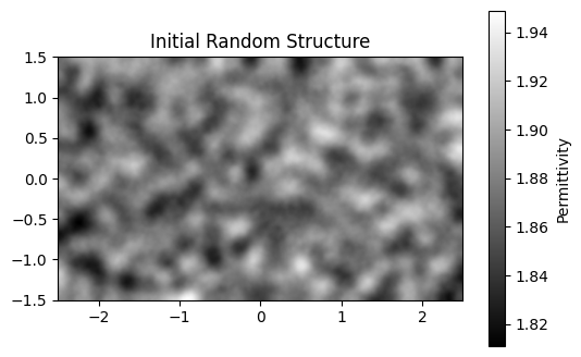
Take a quick look at the initial random permittivity before optimizing.
# Visualization: Initial Structure
print("Plotting Initial Random Permittivity")
eps_initial = get_eps(params0_conv, beta=1).reshape((nx, ny))
plt.figure(figsize=(6, 4))
plt.imshow(np.flipud(eps_initial.T), cmap="gray", origin='lower',
           extent=[-lx_conv / 2, lx_conv / 2, -ly_conv / 2, ly_conv / 2])
plt.colorbar(label="Permittivity")
plt.title("Initial Random Structure")
plt.show()
Plotting Initial Random Permittivity
# Optimization Loop (Mode Converter)
print("Starting Optimization Loop of Mode Converter...")
optimizer_conv = optax.adam(learning_rate=0.3)
params_conv = np.array(params0_conv)
opt_state_conv = optimizer_conv.init(params_conv)
dJ_conv_fn = value_and_grad(J_conv)

beta_history = []
steps_conv = 50

for i in range(steps_conv):
    current_beta = 1.0 + i * 2.0
    beta_history.append(current_beta)

    # Visualization: Iteration Steps
    eps_current = get_eps(params_conv, current_beta).reshape((nx, ny))
    plt.figure(figsize=(4, 2))
    plt.imshow(np.flipud(eps_current.T), cmap="gray", origin='lower')
    plt.title(f"Iteration {i + 1} (Beta={current_beta})")
    plt.axis("off")
    plt.show()

    val, grad = dJ_conv_fn(params_conv, beta=current_beta, step_num=i + 1, verbose=False)
    updates, opt_state_conv = optimizer_conv.update(-grad, opt_state_conv, params_conv)
    params_conv = optax.apply_updates(params_conv, updates)
    params_conv = np.clip(params_conv, 0, 1)
    print(f"Conv Step {i + 1}/{steps_conv} | Beta: {current_beta:.1f} | Obj: {val:.4f}")
Starting Optimization Loop of Mode Converter...
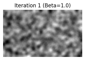
Conv Step 1/50 | Beta: 1.0 | Obj: -0.0999
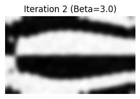
Conv Step 2/50 | Beta: 3.0 | Obj: -0.2121
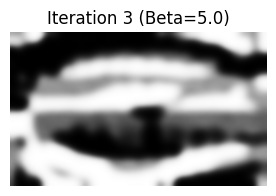
Conv Step 3/50 | Beta: 5.0 | Obj: -0.1902
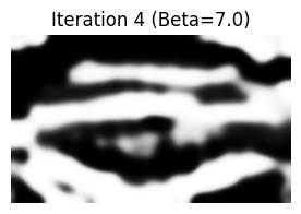
Conv Step 4/50 | Beta: 7.0 | Obj: -0.1413
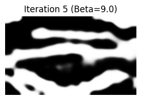
Conv Step 5/50 | Beta: 9.0 | Obj: 0.2045
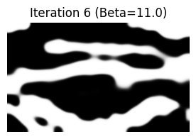
Conv Step 6/50 | Beta: 11.0 | Obj: 0.3171
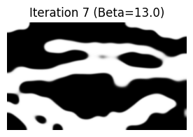
Conv Step 7/50 | Beta: 13.0 | Obj: 0.3817
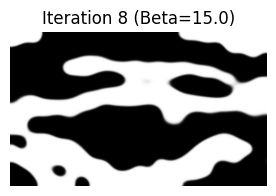
Conv Step 8/50 | Beta: 15.0 | Obj: 0.4103

Conv Step 9/50 | Beta: 17.0 | Obj: 0.4758
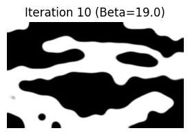
Conv Step 10/50 | Beta: 19.0 | Obj: 0.4965

Conv Step 11/50 | Beta: 21.0 | Obj: 0.5156

Conv Step 12/50 | Beta: 23.0 | Obj: 0.5276

Conv Step 13/50 | Beta: 25.0 | Obj: 0.5566

Conv Step 14/50 | Beta: 27.0 | Obj: 0.5864
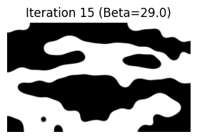
Conv Step 15/50 | Beta: 29.0 | Obj: 0.6000

Conv Step 16/50 | Beta: 31.0 | Obj: 0.6208

Conv Step 17/50 | Beta: 33.0 | Obj: 0.6394

Conv Step 18/50 | Beta: 35.0 | Obj: 0.6532
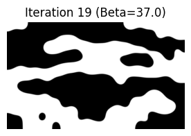
Conv Step 19/50 | Beta: 37.0 | Obj: 0.6691

Conv Step 20/50 | Beta: 39.0 | Obj: 0.6849
Conv Step 21/50 | Beta: 41.0 | Obj: 0.7019

Conv Step 22/50 | Beta: 43.0 | Obj: 0.7152

Conv Step 23/50 | Beta: 45.0 | Obj: 0.7236

Conv Step 24/50 | Beta: 47.0 | Obj: 0.7358

Conv Step 25/50 | Beta: 49.0 | Obj: 0.7457

Conv Step 26/50 | Beta: 51.0 | Obj: 0.7552

Conv Step 27/50 | Beta: 53.0 | Obj: 0.7643

Conv Step 28/50 | Beta: 55.0 | Obj: 0.7728

Conv Step 29/50 | Beta: 57.0 | Obj: 0.7829

Conv Step 30/50 | Beta: 59.0 | Obj: 0.7895

Conv Step 31/50 | Beta: 61.0 | Obj: 0.7933

Conv Step 32/50 | Beta: 63.0 | Obj: 0.7990

Conv Step 33/50 | Beta: 65.0 | Obj: 0.8026

Conv Step 34/50 | Beta: 67.0 | Obj: 0.8069

Conv Step 35/50 | Beta: 69.0 | Obj: 0.8107

Conv Step 36/50 | Beta: 71.0 | Obj: 0.8154

Conv Step 37/50 | Beta: 73.0 | Obj: 0.8190

Conv Step 38/50 | Beta: 75.0 | Obj: 0.8203
Conv Step 39/50 | Beta: 77.0 | Obj: 0.8210

Conv Step 40/50 | Beta: 79.0 | Obj: 0.8242

Conv Step 41/50 | Beta: 81.0 | Obj: 0.8287

Conv Step 42/50 | Beta: 83.0 | Obj: 0.8316
Conv Step 43/50 | Beta: 85.0 | Obj: 0.8354
Conv Step 44/50 | Beta: 87.0 | Obj: 0.8389
Conv Step 45/50 | Beta: 89.0 | Obj: 0.8498

Conv Step 46/50 | Beta: 91.0 | Obj: 0.8662

Conv Step 47/50 | Beta: 93.0 | Obj: 0.8720

Conv Step 48/50 | Beta: 95.0 | Obj: 0.8735

Conv Step 49/50 | Beta: 97.0 | Obj: 0.8737
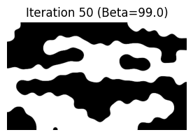
Conv Step 50/50 | Beta: 99.0 | Obj: 0.8761
Final Verification Of The Converter
Rebuild the simulation with the optimized parameters, add a 2D FieldMonitor to visualize the field, and export the binarized structure to GDS.
# Final Verification
sim_final_conv = make_converter_sim(params_conv, beta=beta_history[-1])
field_mnt_conv = td.FieldMonitor(center=(0, 0, 0), size=(td.inf, td.inf, 0), freqs=[freq0], name="field_plot")
sim_final_conv = sim_final_conv.copy(update={"monitors": [field_mnt_conv] + list(sim_final_conv.monitors)})
data_final_conv = web.run(sim_final_conv, task_name="final_conv_verify", verbose=True)
eff_conv = measure_power_conv(data_final_conv)
print(f"Final Converter Efficiency (Mode 2): {eff_conv * 100:.2f}%")
sim_final_conv.to_gds_file("optimized_mode_converter.gds", z=0, permittivity_threshold=(1 + eps_wg) / 2,
                           frequency=freq0)
09:56:49 -03 Created task 'final_conv_verify' with resource_id
             'fdve-5b93d6b2-3902-42bf-b5e4-2a8b512b4953' and task_type 'FDTD'.
             View task using web UI at
             'https://tidy3d.simulation.cloud/workbench?taskId=fdve-5b93d6b2-390
             2-42bf-b5e4-2a8b512b4953'.
Task folder: 'default'.
Output()
09:56:53 -03 Estimated FlexCredit cost: 0.025. Minimum cost depends on task
             execution details. Use 'web.real_cost(task_id)' to get the billed
             FlexCredit cost after a simulation run.
09:56:55 -03 status = success
Output()
09:57:01 -03 Loading results from simulation_data.hdf5
Final Converter Efficiency (Mode 2): 95.00%
Part B: Shape Optimization Of The Output Taper
The taper widens the waveguide from wg_width_conv to w_taper_out while preserving the TE2 mode. Instead of a pixelated density, it is parameterized as a symmetric PolySlab defined by half-widths at a small set of control points along the propagation axis.
A tanh mapping keeps the half-widths between wg_width_conv / 2 and w_taper_out / 2, and a curvature penalty discourages shapes with radii smaller than 0.5 um.
# PART B: TAPER OPTIMIZATION

print(" PART B: TAPER OPTIMIZATION ")

L_taper = 10.0
w_taper_in = wg_width_conv
w_taper_out = 5.0
buffer = 2

Lx_taper_sim = L_taper + 2 * buffer
Ly_taper_sim = w_taper_out + 2 * buffer

num_points = 15
xs = np.linspace(-L_taper / 2, L_taper / 2, num_points)

def get_ys(params):
    p_norm = (anp.tanh(np.pi * params) + 1) / 2
    widths = p_norm * (w_taper_out - w_taper_in) + w_taper_in
    return widths / 2.0

def get_params_from_ys(ys):
    full_widths = ys * 2.0
    p_norm = (full_widths - w_taper_in) / (w_taper_out - w_taper_in)
    p_norm = np.clip(p_norm, 1e-5, 1 - 1e-5)
    return np.arctanh(2 * p_norm - 1) / np.pi
PART B: TAPER OPTIMIZATION
def make_taper_sim(params):
    ys = get_ys(params)
    vertices = anp.concatenate([
        anp.column_stack((xs, ys)),
        anp.column_stack((xs[::-1], -ys[::-1]))
    ])
    taper_geo = td.PolySlab(vertices=vertices, slab_bounds=(-td.inf, td.inf), axis=2)

    taper_struct = td.Structure(geometry=taper_geo, medium=wg_medium)
    wg_in = td.Structure(geometry=td.Box(center=(-L_taper / 2 - buffer / 2, 0, 0), size=(buffer, w_taper_in, td.inf)),
                         medium=wg_medium)
    wg_out = td.Structure(geometry=td.Box(center=(L_taper / 2 + buffer / 2, 0, 0), size=(buffer, w_taper_out, td.inf)),
                          medium=wg_medium)

    mode_spec = td.ModeSpec(num_modes=5)
    source = td.ModeSource(center=(-L_taper / 2 - 1, 0, 0), size=(0, w_taper_in + 4, td.inf),
                           source_time=td.GaussianPulse(freq0=freq0, fwidth=freq0 / 10), direction='+', mode_index=2,
                           mode_spec=mode_spec)
    monitor = td.ModeMonitor(center=(L_taper / 2 + 0.5, 0, 0), size=(0, w_taper_out + 2, td.inf), freqs=[freq0],
                             mode_spec=mode_spec, name="taper_measure")

    return td.Simulation(size=(Lx_taper_sim, Ly_taper_sim, 0),
                         grid_spec=td.GridSpec.auto(min_steps_per_wvl=25, wavelength=wavelength),
                         structures=[wg_in, taper_struct, wg_out], sources=[source], monitors=[monitor],
                         run_time=150 / (freq0 / 10), boundary_spec=td.BoundarySpec.pml(x=True, y=True, z=False))
curvature_penalty = make_curvature_penalty(min_radius=0.5)

def J_taper(params):
    sim = make_taper_sim(params)
    sim_data = web.run(sim, task_name="opt_taper", verbose=False)
    amp = sim_data["taper_measure"].amps.sel(direction="+", f=freq0, mode_index=2).values
    trans = anp.sum(anp.abs(amp) ** 2)
    ys = get_ys(params)
    points = anp.array([xs, ys]).T
    return trans - 5.0 * curvature_penalty(points)
Initialize the taper with a linear ramp from the input to the output half-width and run a short Adam loop. Only a couple of steps are used here because the curvature-regularized linear taper is already a strong starting point; increase num_steps for a longer search.
# Optimization Loop (Taper)
print("Initializing Taper Optimization...")
ys_init = np.linspace(w_taper_in / 2, w_taper_out / 2, num_points)
params_taper = get_params_from_ys(ys_init)

optimizer_taper = optax.adam(learning_rate=0.02)
opt_state_taper = optimizer_taper.init(params_taper)
grad_fn_taper = ag.value_and_grad(J_taper)

for i in range(2):
    params_np = np.array(params_taper)
    val, grad = grad_fn_taper(params_np)
    grad = np.nan_to_num(grad)
    updates, opt_state_taper = optimizer_taper.update(-grad, opt_state_taper, params_taper)
    params_taper = optax.apply_updates(params_taper, updates)
    print(f"Taper Step {i + 1}/2 | Obj: {val:.4f}")
Initializing Taper Optimization...
             WARNING: Warning messages were found in the solver log. For more
             information, check 'SimulationData.log' or use
             'web.download_log(task_id)'.
Taper Step 1/2 | Obj: 0.7787
09:57:06 -03 WARNING: Warning messages were found in the solver log. For more
             information, check 'SimulationData.log' or use
             'web.download_log(task_id)'.
Taper Step 2/2 | Obj: 0.8878
# Final Verification (Taper)
sim_final_taper = make_taper_sim(params_taper)
field_mnt_taper = td.FieldMonitor(center=(0, 0, 0), size=(td.inf, td.inf, 0), freqs=[freq0], name="field_plot")
sim_final_taper = sim_final_taper.copy(update={"monitors": [field_mnt_taper] + list(sim_final_taper.monitors)})
data_final_taper = web.run(sim_final_taper, task_name="final_taper_verify", verbose=True)
eff_taper = float(
    np.sum(np.abs(data_final_taper["taper_measure"].amps.sel(direction="+", f=freq0, mode_index=2).values) ** 2))

print(f"FINAL RESULTS:")
print(f"1. Converter Efficiency (Mode 0 -> 2): {eff_conv * 100:.2f}%")
print(f"2. Taper Efficiency (Mode 2 -> 2):     {eff_taper * 100:.2f}%")

sim_final_taper.to_gds_file("optimized_taper_mode2.gds", z=0, permittivity_threshold=(1 + eps_wg) / 2, frequency=freq0)
09:57:11 -03 Loading simulation from local cache. View cached task using web UI
             at
             'https://tidy3d.simulation.cloud/workbench?taskId=fdve-3d6130e8-064
             e-4b9e-984e-009c9e1142e9'.
             WARNING: Warning messages were found in the solver log. For more
             information, check 'SimulationData.log' or use
             'web.download_log(task_id)'.
FINAL RESULTS:
1. Converter Efficiency (Mode 0 -> 2): 95.00%
2. Taper Efficiency (Mode 2 -> 2):     94.62%
Part C: Combined Device Simulation
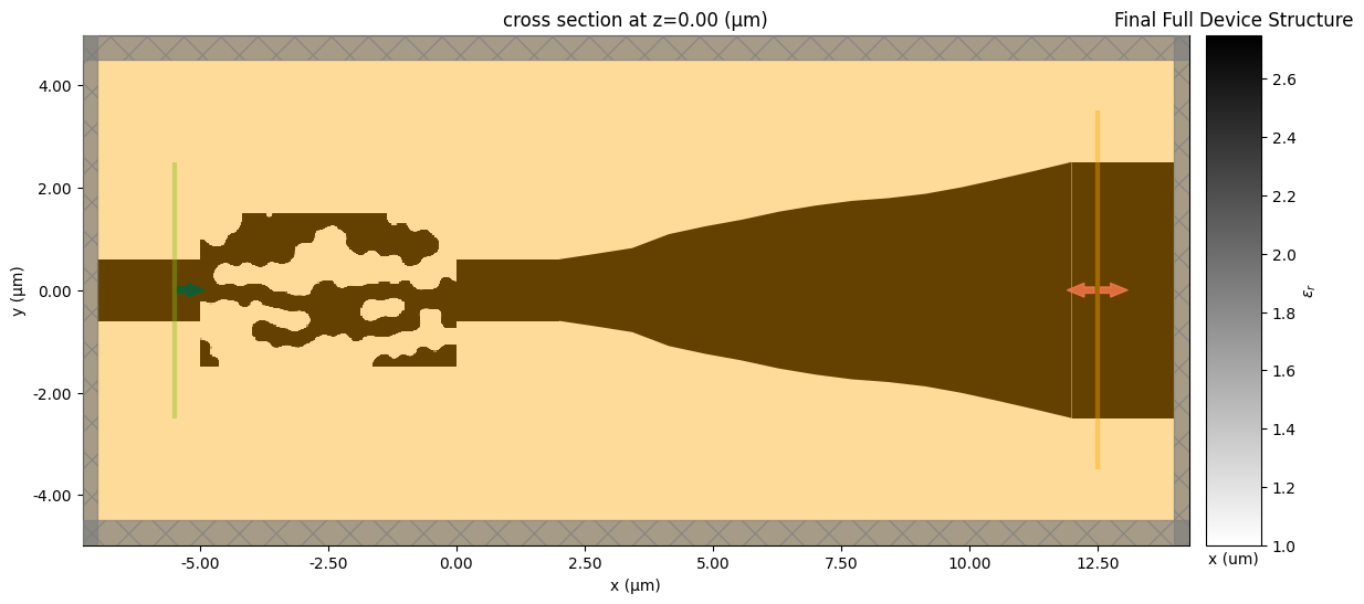
The converter and the taper were optimized in isolation. To confirm the full TE0 -> TE2 launcher, place both optimized structures end to end with a short intermediate waveguide between them and rerun a single combined simulation.
# PART C: FINAL COMBINED SIMULATION (Converter + INTERMEDIATE WG + Taper)

print(" PART C: FINAL COMBINED VERIFICATION ")

mode_spec_final = td.ModeSpec(num_modes=5)

# 1. Converter
# Converter stays at Left: Center = -2.5, Length=5
# Ends at x=0
eps_data_final = get_eps(params_conv, beta=beta_history[-1]).reshape((nx, ny, 1))
converter_geo_final = td.Box(center=(-lx_conv / 2, 0, 0), size=(lx_conv, ly_conv, td.inf))
struct_conv_final = td.Structure.from_permittivity_array(geometry=converter_geo_final, eps_data=eps_data_final)

#  2. Intermediate Waveguide
# Starts at x=0, Ends at x=2 (Length = 2.0 um)
L_mid = 2.0
wg_mid_geo = td.Box(
    center=(L_mid / 2, 0, 0),
    size=(L_mid, wg_width_conv, td.inf)  # Width matches Converter Output & Taper Input
)
struct_wg_mid = td.Structure(geometry=wg_mid_geo, medium=wg_medium)

#  3. Taper
# Previously started at x=0. Now must start at x=L_mid (2.0)
ys_opt = get_ys(params_taper)
xs_shifted = xs + L_taper / 2 + L_mid  # Shift x coordinates by L_taper/2 (to zero) + L_mid

vertices_final = anp.concatenate([
    anp.column_stack((xs_shifted, ys_opt)),
    anp.column_stack((xs_shifted[::-1], -ys_opt[::-1]))
])
taper_geo_final = td.PolySlab(vertices=vertices_final, slab_bounds=(-td.inf, td.inf), axis=2)
struct_taper_final = td.Structure(geometry=taper_geo_final, medium=wg_medium)

#  4. Input & Output Waveguides
wg_in_final = td.Structure(geometry=td.Box(center=(-lx_conv - 1.0, 0, 0), size=(2.0, wg_width_conv, td.inf)),
                           medium=wg_medium)
# Output WG starts at L_mid + L_taper
wg_out_final = td.Structure(geometry=td.Box(center=(L_mid + L_taper + 1.0, 0, 0), size=(2.0, w_taper_out, td.inf)),
                            medium=wg_medium)
PART C: FINAL COMBINED VERIFICATION
#  5. Simulation Setup
Lx_total = lx_conv + L_mid + L_taper + 4.0
sim_center_x = (-lx_conv + L_mid + L_taper) / 2

sim_full = td.Simulation(
    size=(Lx_total, w_taper_out + 4.0, 0),
    center=(sim_center_x, 0, 0),
    grid_spec=td.GridSpec.auto(min_steps_per_wvl=25, wavelength=wavelength),
    structures=[wg_in_final, struct_conv_final, struct_wg_mid, struct_taper_final, wg_out_final],
    sources=[td.ModeSource(center=(-lx_conv - 0.5, 0, 0), size=(0, ly_conv + 2, td.inf),
                           source_time=td.GaussianPulse(freq0=freq0, fwidth=freq0 / 10), direction='+', mode_index=0,
                           mode_spec=mode_spec_final)],
    monitors=[td.ModeMonitor(center=(L_mid + L_taper + 0.5, 0, 0), size=(0, w_taper_out + 2, td.inf), freqs=[freq0],
                             mode_spec=mode_spec_final, name="full_measure"),
              td.FieldMonitor(center=(sim_center_x, 0, 0), size=(td.inf, td.inf, 0), freqs=[freq0], name="field_plot")],
    run_time=200 / (freq0 / 10),
    boundary_spec=td.BoundarySpec.pml(x=True, y=True, z=False)
)

#  VISUALIZATION of Final Device
print("Plotting Final Full Device Structure")
fig, ax = plt.subplots(figsize=(15, 6))
sim_full.plot_eps(z=0, ax=ax)
plt.title("Final Full Device Structure")
plt.xlabel("x (um)")
plt.show()
Plotting Final Full Device Structure
print("Running Full Combined System...")
data_full = web.run(sim_full, task_name="full_device_simulation", verbose=True)
amp_full = data_full["full_measure"].amps.sel(direction="+", f=freq0, mode_index=2).values
eff_full = float(np.sum(np.abs(amp_full) ** 2))
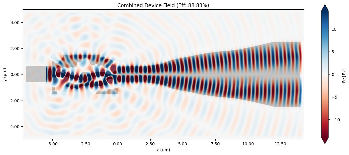
print(f"TOTAL SYSTEM EFFICIENCY: {eff_full * 100:.2f}%")
fig, ax = plt.subplots(figsize=(15, 6))
data_full.plot_field("field_plot", "Ez", z=0, ax=ax)
plt.title(f"Combined Device Field (Eff: {eff_full * 100:.2f}%)")
plt.xlabel("x (um)")
plt.show()
sim_full.to_gds_file("Final_Full_Device_Mode0_to_Mode1_to_Taper.gds", z=0, permittivity_threshold=(1 + eps_wg) / 2, frequency=freq0)
print("Saved 'Final_Full_Device_Mode0_to_Mode1_to_Taper.gds'")
Running Full Combined System...
09:57:12 -03 Created task 'full_device_simulation' with resource_id
             'fdve-fdcc24c4-44fa-4c70-87c6-035a04bc82cf' and task_type 'FDTD'.
             View task using web UI at
             'https://tidy3d.simulation.cloud/workbench?taskId=fdve-fdcc24c4-44f
             a-4c70-87c6-035a04bc82cf'.
Task folder: 'default'.
Output()
09:57:16 -03 Estimated FlexCredit cost: 0.025. Minimum cost depends on task
             execution details. Use 'web.real_cost(task_id)' to get the billed
             FlexCredit cost after a simulation run.
09:57:18 -03 status = success
Output()
09:57:32 -03 Loading results from simulation_data.hdf5
             WARNING: Warning messages were found in the solver log. For more
             information, check 'SimulationData.log' or use
             'web.download_log(task_id)'.
TOTAL SYSTEM EFFICIENCY: 88.83%
Saved 'Final_Full_Device_Mode0_to_Mode1_to_Taper.gds'