Author: Leyang Liu, University of Illinois Urbana-Champaign
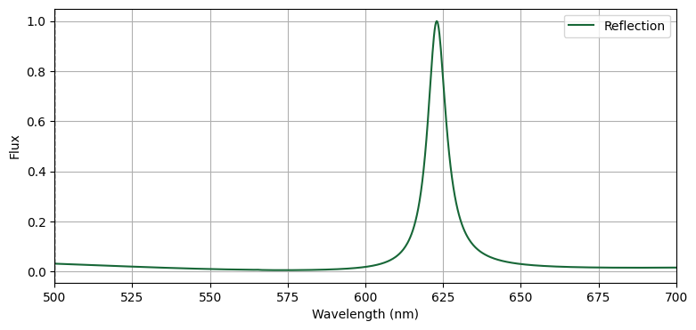
In this notebook, we simulate the optical reflection spectrum of a 1D photonic crystal / grating structure using Tidy3D. The structure consists of patterned SiO₂ and TiO₂ layers embedded in polymer (PVA) on a substrate. A broadband plane wave is incident on the structure, and the notebook computes:
- Reflection spectrum vs wavelength
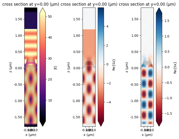
- Electric field distribution
- Poynting vector flow
This type of simulation is typical for biosensors, dielectric metasurfaces, or photonic crystal reflectors.
[1]:
import matplotlib.pyplot as plt
import numpy as np
import tidy3d as td
import tidy3d.web as web
from tidy3d.plugins.dispersion import FastDispersionFitter
15:53:46 UTC WARNING: Using canonical configuration directory at
             '/home/tidy3d/.config/tidy3d'. Found legacy directory at
             '~/.tidy3d', which will be ignored. Remove it manually or run
             'tidy3d config migrate --delete-legacy' to clean up.
Define material properties:
[2]:
# materials
SiO2 = td.Medium(
    name = 'SiO2',
    permittivity = 2.1025,
)
TiO2 = td.Medium(
    name = 'TiO2',
    permittivity = 5.8081000000000005,
)
background = td.Medium(permittivity=1**2)
PVA = td.Medium(permittivity = 1.483**2)
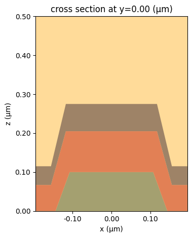
Define structure geometry:
[3]:
period = 0.39
TiO2_thick = 0.105
SiO2_thick = 0.1
PVA_thick = 0.070
PVA_bottom_thick = 0.048
sub_thick = 2
monitor_distance = 1.0
monitor_gap = 0.1
dutycycle_SiO2 = 0.55
TiO2_bottom_thick = 0.067
slope_angle = 70/180*np.pi
dutycycle_TiO2 = 0.6
size_z = sub_thick+SiO2_thick+TiO2_thick+monitor_distance+monitor_gap
SiO2_top_width = dutycycle_SiO2*period
SiO2_bottom_width = SiO2_top_width+2*SiO2_thick/np.tan(slope_angle)
TiO2_top_width = dutycycle_TiO2*period
TiO2_bottom_width = TiO2_top_width+2*TiO2_thick/np.tan(slope_angle)
Define simulation parameters:
[4]:
# the epoxy layer top surface is at z=0
sim_center = (0, 0, 0)
sim_size = (
    period,
    0,
    size_z
)

# wavelength / frequency setup
nm = 1e-3
wavelength_min = 500 * nm
wavelength_max = 700 * nm
freq_min = td.C_0 / wavelength_max
freq_max = td.C_0 / wavelength_min
freq0 = td.C_0 / (500 * nm)
fwidth = freq_max - freq_min
run_time = 10e-11

# SiO2 sub
SiO2_sub = td.Structure(
    geometry=td.Box(
        center=[0.0, 0.0, -0.5 * sub_thick],
        size=[td.inf, td.inf, sub_thick],
    ),
    medium=SiO2,
    name="SiO2_sub",
)

# SiO2 teeth
vertices1 = [[SiO2_bottom_width / 2, 0],
    [-SiO2_bottom_width / 2, 0],
    [-SiO2_top_width / 2, SiO2_thick],
    [SiO2_top_width / 2, SiO2_thick]]
SiO2_teeth = td.Structure(
    geometry = td.PolySlab(axis = 1, slab_bounds = [-td.inf, td.inf], vertices = vertices1),
    name = 'SiO2_teeth',
    medium = SiO2
)

# TiO2
vertices2 = [[TiO2_bottom_width / 2, TiO2_bottom_thick],
    [TiO2_top_width / 2, SiO2_thick + TiO2_thick],
    [-TiO2_top_width / 2, SiO2_thick + TiO2_thick],
    [-TiO2_bottom_width / 2, TiO2_bottom_thick],
    [-period / 2, TiO2_bottom_thick],
    [-period / 2, 0],
    [-SiO2_bottom_width / 2, 0],
    [-SiO2_top_width / 2, SiO2_thick],
    [SiO2_top_width / 2, SiO2_thick],
    [SiO2_bottom_width / 2, 0],
    [period / 2, 0],
    [period / 2, TiO2_bottom_thick]]
TiO2 = td.Structure(
    geometry = td.PolySlab(axis = 1, slab_bounds = [-td.inf, td.inf], vertices = vertices2),
    medium = TiO2,
    name = 'TiO2'
)

# PVA
vertices3 = [[TiO2_bottom_width / 2, TiO2_bottom_thick + PVA_bottom_thick],
    [TiO2_top_width / 2, SiO2_thick + TiO2_thick + PVA_thick],
    [-TiO2_top_width / 2, SiO2_thick + TiO2_thick + PVA_thick],
    [-TiO2_bottom_width / 2, TiO2_bottom_thick + PVA_bottom_thick],
    [-period / 2, TiO2_bottom_thick + PVA_bottom_thick],
    [-period / 2, TiO2_bottom_thick],
    [-TiO2_bottom_width / 2, TiO2_bottom_thick],
    [-TiO2_top_width / 2, SiO2_thick + TiO2_thick],
    [TiO2_top_width / 2, SiO2_thick + TiO2_thick],
    [TiO2_bottom_width / 2, TiO2_bottom_thick],
    [period / 2, TiO2_bottom_thick],
    [period / 2, TiO2_bottom_thick + PVA_bottom_thick]]
PVA = td.Structure(
    geometry = td.PolySlab(axis = 1, slab_bounds = [-td.inf, td.inf], vertices = vertices3),
    medium = PVA,
    name = 'PVA'
)

# the order here matters, because the teeth must override the bottom film layer
geometry = [SiO2_sub, SiO2_teeth, TiO2, PVA]
# geometry = [epoxy_layer, bottom_film, grating_teeth, top_film]
# boundary conditions: the simulation is periodic in the x-y plane, and simulates
# an infinite domain along z
boundary_spec = td.BoundarySpec(
    x=td.Boundary.periodic(),
    y=td.Boundary.periodic(),
    z=td.Boundary.pml(),
)

# grid specification
grid_spec = td.GridSpec.auto(min_steps_per_wvl=30)
Define source:
[5]:
source_time = td.GaussianPulse(freq0=freq0, fwidth=fwidth)
source = td.PlaneWave(
    center=[0, 0, TiO2_thick + SiO2_thick + monitor_distance],
    size=[td.inf, td.inf, 0.0],
    source_time=source_time,
    pol_angle=0,
#    pol_angle=np.pi/2,
    direction="-",
    angle_theta=np.deg2rad(0),
    angular_spec=td.FixedAngleSpec(),
)
Define monitors:
[6]:
# create field monitor
monitor_xz = td.FieldMonitor(
    center=sim_center,
    size=[td.inf, 0, td.inf],
    freqs=[freq0],
    name="fields_xz",
)

# create flux monitors
freqs = np.linspace(freq_min, freq_max, 1000)
monitor_flux_refl = td.FluxMonitor(
    center=[0, 0, monitor_distance],
    size=[td.inf, td.inf, 0.0],
    freqs=freqs,
    name="flux_refl",
)
monitors = [monitor_xz, monitor_flux_refl]
Put everything together in a simulation object:
[7]:
# create the simulation
sim = td.Simulation(
    center=sim_center,
    size=sim_size,
    grid_spec=grid_spec,
    structures=geometry,
    sources=[source],
    monitors=monitors,
    run_time=run_time,
    boundary_spec=boundary_spec,
    medium=background,
    shutoff=1e-7,
)

# plot the simulation domain
#sim.plot_3d()
#plt.show()
sim.plot(y=0.0, vlim=[0, 0.5])
plt.show()
15:53:49 UTC WARNING: Structure at 'structures[2]' has bounds that extend
             exactly to simulation edges. This can cause unexpected behavior. If
             intending to extend the structure to infinity along one dimension,
             use td.inf as a size variable instead to make this explicit.
WARNING: Suppressed 3 WARNING messages.
[8]:
import tidy3d.web as web

sim_data = web.run(sim, task_name="biosensor", path="data/biosensor.hdf5", verbose=True)
             WARNING: Simulation has 6.33e+06 time steps. The 'run_time' may be
             unnecessarily large, unless there are very long-lived resonances.
             Created task 'biosensor' with resource_id
             'fdve-9878e97e-7c50-4fd4-8631-65f84387e98b' and task_type 'FDTD'.
             View task using web UI at
             'https://tidy3d.simulation.cloud/workbench?taskId=fdve-9878e97e-7c5
             0-4fd4-8631-65f84387e98b'.
Task folder: 'default'.
Output()
15:53:50 UTC Estimated FlexCredit cost: 0.040. Minimum cost depends on task
             execution details. Use 'web.real_cost(task_id)' to get the billed
             FlexCredit cost after a simulation run.
status = success
Output()
15:53:51 UTC Loading simulation from data/biosensor.hdf5
             WARNING: Structure at 'structures[2]' has bounds that extend
             exactly to simulation edges. This can cause unexpected behavior. If
             intending to extend the structure to infinity along one dimension,
             use td.inf as a size variable instead to make this explicit.
WARNING: Suppressed 3 WARNING messages.
             WARNING: Warning messages were found in the solver log. For more
             information, check 'SimulationData.log' or use
             'web.download_log(task_id)'.
[9]:
fig, ax = plt.subplots(1, 3, figsize=(8, 6), tight_layout=True)

sim_data.plot_field("fields_xz", field_name="E", val="abs", f=freq0, ax=ax[0])
sim_data.plot_field("fields_xz", field_name="Sz", val="real", f=freq0, ax=ax[1])
sim_data.plot_field("fields_xz", field_name="Sx", val="real", f=freq0, ax=ax[2])
plt.show()
[10]:
reflection = sim_data["flux_refl"].flux+1

fig, ax = plt.subplots(figsize=(9, 4))

ax.plot(td.C_0 / freqs * 1e3, reflection, label="Reflection")

# wavelength for the field plots
ax.axvline(td.C_0 / freq0 * 1e3, ls="--", color="k", lw=1)

ax.set(
    xlabel="Wavelength (nm)",
    ylabel="Flux",
    xlim=(wavelength_min * 1e3, wavelength_max * 1e3),
)
ax.legend()
ax.grid()
#plt.xlim(550, 650)
plt.show()
[11]:
#fig.savefig("1degree_30.tif", dpi=300)
[ ]: