





Author: Edward B. Flagg, West Virginia University
Summary
An epitaxial quantum dot generally has two orthogonal linearly polarized transition dipole moments, one for each of the two confined exciton states. This notebook uses several complementary inverse design approaches to produce a photonic device that will cause the two dipole moments to emit light into separate waveguides. Since the device separates different photon polarization states, we call it a "polarization demultiplexer" or "poldemux". The resulting design looks like this:
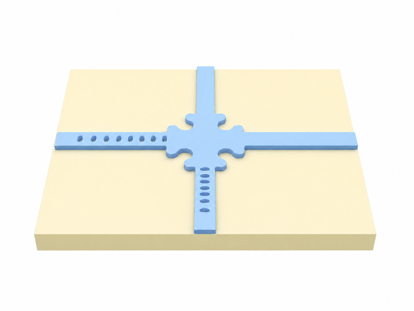
We will use a shape-optimization approach rather than a topology-optimization approach because it produces eminently fabricable designs at every step in the process. There are two main components to the design that will be optimized:
- Waveguide crossing (WGX): The design comprises four waveguides intersecting at right angles, with a crossing region whose border can be varied. A linearly polarized dipole source is located at the center of the crossing region and the origin of the simulation region. The shape of the WGX will be optimized to maximize the coupling of the dipole source into two output waveguides and to minimize the coupling into the other two waveguides (i.e., to minimize the crosstalk).
- Photonic crystal (PhC) mirror: Two of the waveguides will contain photonic crystal mirrors to back-reflect the emission, so the light from one linearly polarized dipole only exits one output waveguide.
Since the device performance is determined by the outer border of the WGX, the design is suitable for a sleeve-and-bulk fabrication process. This is advantageous because sleeve-and-bulk fabrication can produce multiple device designs in the same run without multiple rounds of process optimization.
The symmetry of the device is such that only one linearly polarized dipole needs to be simulated. If the device is optimized to maximize the coupling efficiency of one dipole into one output waveguide, then the enforced symmetry guarantees that the orthogonal dipole will be equivalently coupled to the other output waveguide.
Optimization Approaches Used
Gradient-based approaches to maximizing an objective function work well to improve an initial design, but can only produce high-performing devices if the design starts in a convex region of parameter space containing a good maximum. We have found that gradient-based optimization functions best with a good starting design. In order to find a good initial design, a gradient-free heuristic optimization in a lower-dimensional parameter space is an appropriate approach. Thus, the design will proceed in several stages:
Stage 1: Bayesian optimization (BO) of the WGX with a low-dimensional parameterization of the border. The purpose of this stage is to find a good initial design for later refinement via adjoint optimization. The design produced by this step will be resampled to find initial control points representing the border to use for adjoint optimization.
Stage 2: Adjoint optimization of the WGX border parameterized using the control points of an interpolating spline.
Stage 3: Bayesian optimization (BO) of the photonic crystal mirrors with a low-dimensional parameterization of the mirror holes.
Stage 4: Simultaneous adjoint optimization of the WGX border and photonic crystal mirror holes.
BO enables exploration of a larger design space than gradient-based adjoint optimization does, so it is an appropriate approach to find a suitable initial design whence to begin adjoint optimization. Another gradient-free heuristic approach, such as particle-swarm optimization, might work as well. An advantage to BO is that it allows one to choose whether the algorithm explores unknown regions of parameter space or exploits the current knowledge of parameter space to find optimum designs. Since the BO design will be later optimized with a gradient-based approach, it is unnecessary to find the optimum design during the BO step. Thus, we have chosen BO with parameters that prefer exploration rather than exploitation.
Since close proximity to etched surfaces can produce detrimental spectral diffusion in quantum dots, a border-distance penalty is included in the objective function at each stage of the design process to prevent the border from getting too close to the dipole source. Previous research has determined that 300 nm is an appropriate minimum proximity to limit the effects of spectral diffusion.
Imports
# Standard python imports
import matplotlib.pylab as plt
import numpy as np

# Import regular tidy3d
import tidy3d as td
import tidy3d.web as web

# Import tidy3d plugins
from tidy3d.plugins.autograd import (
    interpolate_spline,
    make_curvature_penalty,
    value_and_grad,
)
import tidy3d.plugins.design as tdd

# Import autograd.numpy for adjoint gradient
import autograd.numpy as anp

# Import optax for optimization
import optax

# Supplemental imports
import pickle  # For saving metadata and optimization progress
from pathlib import Path
from tqdm.auto import tqdm  # For displaying progress bar in FOR loop
from shapely import LineString  # For detecting polygon self-intersection

plt.rcParams["font.size"] = "12"
Static Design Parameters
These are the same regardless of the device design.
# Dipole source parameters
wl = 0.798  # Central simulation wavelength (um).
bw = 0.020  # Simulation bandwidth (um), i.e., the full spectral width.
n_wl = 81  # Number of wavelength points within the bandwidth.
center_idx = n_wl // 2  # Index for the design (i.e., central) wavelength
run_time = 0.5e-12  # ps.    For a resonant structure, 2e-12 or 5e-12 might work better.

# Physical parameters
wg_height = 0.150  # microns, thickness of membrane containing the dipole
wg_width = 0.300  # microns, width of the output waveguides
wg_length = 3.0  # microns
origin = (0, 0, 0)

# Calculated wavelengths and frequencies
wl_max = wl + bw / 2
wl_min = wl - bw / 2
wl_range = anp.linspace(wl_min, wl_max, n_wl)
freq0 = td.C_0 / wl
freqs = td.C_0 / wl_range
freqhw = 0.5 * (freqs[0] - freqs[-1])
AlGaAs Refractive Index
The refractive index of the AlGaAs membrane wherein sits the dipole is calculated using the model in the following paper:
Langer M, Dhurjati SA, Bauer M, Zena YG, Rahimi A, Bassoli R, Fitzek FHP, Schmidt OG, Hopfmann C (2025). "Temperature-dependent refractive index of AlGaAs for quantum-photonic devices near the bandgap." https://doi.org/10.48550/arXiv.2512.02212
# Relevant parts of Adachi model; Eqn. (3) in Langer et al.
def E0(x):
    # Room temp band gap at Gamma point.
    # Eqn. (23) or Table II in Adachi, J. Appl. Phys. 1985.
    return 1.425 + 1.155 * x + 0.37 * x**2  # in eV


def E0andDelta0(x):
    # From Table II in Adachi, J. Appl. Phys. 1985.
    # Delta0 is the energy difference between the Gamma point and the split-off band,
    # which is related to the spin-orbit energy.
    return 1.765 + 1.155 * x + 0.37 * x**2  # in eV


def chi(wavelength, gap):
    # Ratio between photon energy at 'wavelength' and the band gap
    # gap must be in eV
    # If wavelength = 1, this returns the wavelength of the band edge in microns
    hc = 1.240  # eV*um, Planck's constant times the speed of light
    return hc / wavelength / gap


def f(chivalue):
    # np.emath.sqrt() deals correctly with negative arguments
    return (2 - np.emath.sqrt(1 + chivalue) - np.emath.sqrt(1 - chivalue)) / chivalue**2


# Varshni/Vurgaftman temperature-dependent model for band gap.
# Eqn. (1) in Langer et al.
def alpha(x):
    return (5.405 * (1 - x) + 8.85 * x) * 1e-4  # eV/K


def beta(x):
    return 204 * (1 - x) + 530 * x  # in K


def E0_0K(x):
    # Band gap at T = 0 K
    return 1.519 + 1.155 * x + 0.37 * x**2  # eV


def Egap(x, temp):
    return E0_0K(x) - alpha(x) * temp**2 / (temp + beta(x))


# Langer et al. model; Eqn. (4) in Langer et al.
def A0prime(x):
    return 6.741 + 2.938 * x + 11.686 * x**2


def B0prime(x):
    return 9.275 - 2.489 * x - 6.940 * x**2


C0 = -2.618e-6  # K^-1
D0 = 4.282e-7  # K^-2


def index_adachi_temp_dependent(x, wavelength, temp):
    # Eqn. (3) in Langer et al. with a temperature-dependent band edge shift via Eqn. (1).
    return np.sqrt(
        A0prime(x)
        * (
            f(chi(wavelength, Egap(x, temp)))
            + f(chi(wavelength, E0andDelta0(x)))
            / 2
            * (Egap(x, temp) / E0andDelta0(x)) ** (3 / 2)
        )
        + B0prime(x)
    )


def AlGaAsIndex(x, wavelength, temp):
    """
    x = Al/Ga alloy fraction for Al_x Ga_(1-x) As [unitless]
    wavelength [um]
    temp = temperature [K]

    returns the index of refraction (in general complex)
    """
    return index_adachi_temp_dependent(x, wavelength, temp) + C0 * temp + D0 * temp**2


# Media parameters
alloy_fraction = 0.13  # Al fraction in the AlGaAs medium
temperature = 4  # Operating temperature of the device (in Kelvin)
n_AlGaAs = AlGaAsIndex(alloy_fraction, wl, temperature)
AlGaAs_simple = td.Medium(permittivity=n_AlGaAs**2)
vacuum = td.Medium(permittivity=1)
Stage 1: BO of WGX
This section of the notebook will cost approximately 2.5 flexcredits and take about 2.25 hours to run.WGX Border Parameterization: B-splines
We choose B-splines to parameterize the border of the WGX for two reasons: (1) It only requires a few control points to allow a large space of structure designs, which is important for a Bayesian optimization approach. (2) B-splines satisfy the convex hull property, which means the spline is always inside the polygon formed by the control points. Thus, by bounding the allowed positions of the control points we also ensure that the spline doesn't extend outside the allowed region. Interpolating splines like natural cubic splines do not have that guarantee. That is why for this stage we do not use the built-in function tidy3d.plugins.autograd.interpolate_spline.
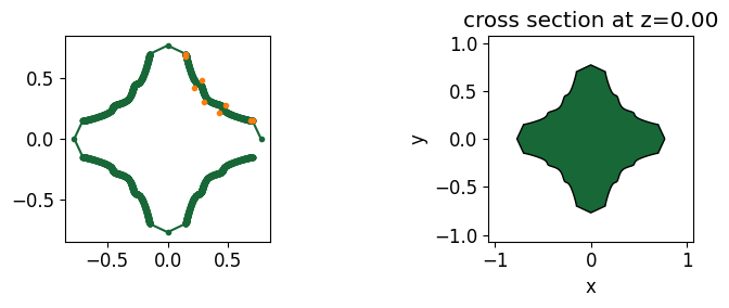
The device is expected to have $C_{4v}$ symmetry, which is the symmetry group of a square. It comprises four-fold rotational symmetry and four mirror planes, which means that only 1/8th of the border is needed to determine the entire WGX shape. The 1/8th border is parameterized using three variable control points: two free points and one point confined to the diagonal line $y=x$. The two free points must still be confined within the triangle formed by the edge of the allowed WGX region, the edge of the output waveguide, and the diagonal symmetry line. An $(x,y)$ position in this triangular two-dimensional region can be represented using three barycentric coordinates, which are in turn derived from two design coordinates bounded in the domain $[0, 1]$.
cross_width = 1.40  # microns.
num_free_pts = 2  # in 1/8th of the device border, not counting the diagonal point
smidge = 0.020  # A small distance offset helpful to ensure the spline joins the waveguide smoothly
vertex_spacing = 0.001  # microns

# Waveguide corners and boundary corners of the allowed control-point region
wg_corner1 = anp.array([cross_width / 2, wg_width / 2])
wg_corner2 = anp.array([cross_width / 2 - smidge, wg_width / 2])
inner_corner = anp.array([wg_corner1[1], wg_corner1[1]])
outer_corner = anp.array([wg_corner1[0], wg_corner1[0]])
diag_min = wg_corner1[1]
diag_max = wg_corner1[0] * 0.75


def barycentric_from_2d(u, v):
    """Convert bounded 2D design coords to barycentric coords."""
    t0 = 1 - u
    t1 = u * (1 - v)
    t2 = u * v
    return (t0, t1, t2)


def ctrl_pt_from_barycentric(bary_coords, corner0, corner1, corner2):
    """Convert barycentric coords into (x,y) coords given the bounding corners of a triangle."""
    t0, t1, t2 = bary_coords
    P = t0 * corner0 + t1 * corner1 + t2 * corner2
    return P


def ctrl_pt_array_from_params(params, corner0, corner1, corner2):
    """
    Given bounded design parameters and corners of the control-point triangle,
    return an array of control points for the first quarter of the WGX border.
    """
    u1, v1, u2, v2, d = params
    a_bit = 1e-3
    # Check if any of the following equalities hold.
    # If so, avoid self-intersection in the spline by changing one design parameter by a bit.
    if u1 == u2:
        if u1 == 0:
            u2 = u2 + a_bit
        if u1 == 1:
            u2 = u2 - a_bit
    if v1 == v2:
        if v1 == 0:
            v2 = v2 + a_bit
        if v1 == 1:
            v2 = v2 - a_bit

    bary1 = barycentric_from_2d(u1, v1)
    bary2 = barycentric_from_2d(u2, v2)
    free_point1 = ctrl_pt_from_barycentric(bary1, corner0, corner1, corner2)
    free_point2 = ctrl_pt_from_barycentric(bary2, corner0, corner1, corner2)
    diag_point = anp.array([d, d])

    # Detect and correct self-intersection
    polyline = LineString(
        coordinates=anp.array([wg_corner2, free_point1, free_point2, diag_point])
    )
    if polyline.is_simple:  # then proceed with points in order
        ctrl_pts = anp.array(
            [
                wg_corner1,
                wg_corner2,
                free_point1,
                free_point2,
                diag_point,
                free_point2[::-1],
                free_point1[::-1],  # Mirrored across the diagonal
                wg_corner2[::-1],
                wg_corner1[::-1],
            ]
        )  # Mirrored across the diagonal
    else:  # avoid self-intersection by switching the order of the two free points
        ctrl_pts = anp.array(
            [
                wg_corner1,
                wg_corner2,
                free_point2,
                free_point1,
                diag_point,
                free_point1[::-1],
                free_point2[::-1],  # Mirrored across the diagonal
                wg_corner2[::-1],
                wg_corner1[::-1],
            ]
        )  # Mirrored across the diagonal

    return ctrl_pts  # for one-quarter of the device border


def nik(i, k, t, knots):
    """Basis functions for a B-spline of degree k."""
    assert isinstance(i, int) & (i >= 0), "i must be a non-negative integer"
    assert isinstance(k, int) & (k >= 0), "k must be a non-negative integer"
    assert i + k + 1 < len(knots), (
        "i+k+1 must be less than the length of the knot vector"
    )

    if k == 0:
        values = anp.zeros_like(t)
        values[(knots[i] <= t) & (t < knots[i + 1])] = 1
        return values

    # To avoid divide-by-zero errors, find the basis functions before deciding whether to calculate the coefficients.
    basis1 = nik(i, k - 1, t, knots)
    basis2 = nik(i + 1, k - 1, t, knots)
    if all(basis1 == 0):
        c1 = 0
    else:
        c1 = (t - knots[i]) / (knots[i + k] - knots[i])
    if all(basis2 == 0):
        c2 = 0
    else:
        c2 = (knots[i + k + 1] - t) / (knots[i + k + 1] - knots[i + 1])
    return c1 * basis1 + c2 * basis2


def calc_basis_funcs(k=3, num_control_pts=None, vertex_spacing=0.001):
    """Calculate and return the array of basis functions"""
    # Knots
    n = num_control_pts - 1
    interior_knots = anp.linspace(
        0, 1, n - k + 2
    )  # knot values are all in the range [0,1].
    knots = anp.concatenate(
        (anp.zeros(k), interior_knots, anp.ones(k) * interior_knots[-1])
    )

    # Basis functions
    times = anp.arange(knots[0], knots[-1], vertex_spacing)
    basis_funcs = []
    for i in range(0, n + 1):
        basis_funcs.append(nik(i, k, times, knots))
    basis_funcs = anp.array(basis_funcs)

    return basis_funcs


def make_border_vertices(basis_funcs, control_points):
    """Returns the vertices for the upper-right border of the WGX."""
    quarter_border_vertices = basis_funcs.T @ control_points
    return quarter_border_vertices


def border_vertices_to_all(quarter_border_vertices):
    """Returns the vertices of the whole cross region given those of the upper-right quarter."""

    # Single points at the tip of each arm of the WGX ensure it attaches to the waveguides.
    pin_factor = 1.1  # Depth into the waveguide of the point
    right_point = anp.array([[cross_width / 2 * pin_factor, 0]])
    top_point = anp.array([[0, cross_width / 2 * pin_factor]])
    left_point = anp.array([[-cross_width / 2 * pin_factor, 0]])
    bot_point = anp.array([[0, -cross_width / 2 * pin_factor]])

    reflect_in_x = anp.array([-1, 1])
    inversion = anp.array([-1, -1])

    upper_right = quarter_border_vertices
    upper_left = (reflect_in_x * upper_right)[::-1]
    lower_left = inversion * upper_right
    lower_right = inversion * upper_left

    vertices = anp.concatenate(
        [
            right_point,
            upper_right,
            top_point,
            upper_left,
            left_point,
            lower_left,
            bot_point,
            lower_right,
        ]
    )

    return vertices


# Basis functions will be precalculated once because they don't change unless the number of control points changes.
basis_funcs = calc_basis_funcs(
    k=3, num_control_pts=2 * num_free_pts + 5, vertex_spacing=vertex_spacing
)


def make_vertices(params):
    """Return the WGX vertices given the design parameters."""
    ctrl_pts = ctrl_pt_array_from_params(params, inner_corner, outer_corner, wg_corner1)
    quarter_border_vertices = make_border_vertices(basis_funcs, ctrl_pts)
    vertices = border_vertices_to_all(quarter_border_vertices)
    return vertices


# Helper functions
def make_polyslab(params: anp.ndarray) -> td.PolySlab:
    """Make a `tidy3d.PolySlab` for the device given the design parameters."""
    vertices = make_vertices(params)
    return td.PolySlab(
        vertices=vertices, slab_bounds=(-wg_height / 2, wg_height / 2), axis=2
    )


def make_structure(params) -> td.Structure:
    """Make a `tidy3d.Structure` for the device given the design parameters."""
    cross_polyslab = make_polyslab(params)
    return td.Structure(geometry=cross_polyslab, medium=AlGaAs_simple)


# Test out the above approach with arbitrarily chosen parameters.
initial_params = [0.5, 0.75, 0.6, 0.6, 0.3]
# initial_params = [0, 1, 0, 1, 0.5] # a test for self-intersections

fig1, (ax1, ax2) = plt.subplots(1, 2, figsize=(8, 3), tight_layout=True)
ctrl_pts = ctrl_pt_array_from_params(
    initial_params, inner_corner, outer_corner, wg_corner1
)
vertices = make_vertices(initial_params)
ax1.plot(*vertices.T, ".-")
ax1.plot(*ctrl_pts.T, ".")
ax1.set_aspect("equal")

cross_polyslab = make_polyslab(initial_params)
ax2 = cross_polyslab.plot(z=0, ax=ax2)
plt.show()
Static Structures
Define the static geometries like the four input/output waveguides. These are not affected by the design parameters of the WGX.
right_wg_box = td.Box(
    center=((cross_width + wg_length) / 2, 0, 0), size=(wg_length, wg_width, wg_height)
)
top_wg_box = td.Box(
    center=(0, (cross_width + wg_length) / 2, 0), size=(wg_width, wg_length, wg_height)
)
left_wg_box = td.Box(
    center=(-(cross_width + wg_length) / 2, 0, 0), size=(wg_length, wg_width, wg_height)
)
bot_wg_box = td.Box(
    center=(0, -(cross_width + wg_length) / 2, 0), size=(wg_width, wg_length, wg_height)
)

right_wg = td.Structure(geometry=right_wg_box, medium=AlGaAs_simple, name="right wg")
top_wg = td.Structure(geometry=top_wg_box, medium=AlGaAs_simple, name="top wg")
left_wg = td.Structure(geometry=left_wg_box, medium=AlGaAs_simple, name="left wg")
bot_wg = td.Structure(geometry=bot_wg_box, medium=AlGaAs_simple, name="bot wg")

static_structures = [right_wg, top_wg, left_wg, bot_wg]
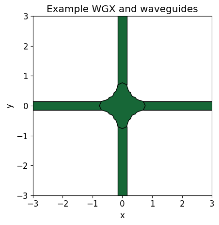
Plot the polyslabs all together so we can check that they overlap.
ax = right_wg_box.plot(z=0)
top_wg_box.plot(z=0, ax=ax)
left_wg_box.plot(z=0, ax=ax)
bot_wg_box.plot(z=0, ax=ax)
cross_polyslab.plot(z=0, ax=ax)
ax.set_xlim([-3, 3])
ax.set_ylim([-3, 3])
ax.set_title("Example WGX and waveguides")
plt.show()
Define Simulation
Simulation Specifications
Some aspects of the simulation will be the same regardless of the design parameters. We define those uniform specifications here.
# Simulation specifications
source_time = td.GaussianPulse(freq0=freq0, fwidth=freqhw)
grid_spec = td.GridSpec.auto(wavelength=wl, min_steps_per_wvl=15)
boundary_spec = td.BoundarySpec.all_sides(boundary=td.PML())

# Symmetry choices
# When the device has C_4v symmetry with a y-polarized dipole at the origin,
# the symmetry requires PMC on z=0 and x=0, PEC on y=0,
symmetry_A = (1, -1, 1)
# When two waveguides have mirrors, there is only PMC symmetry at z=0.
symmetry_B = (0, 0, 1)  # PMC symmetry on z=0 plane; E_perp = 0, H_parallel = 0

# Source
dipole_src = td.PointDipole(center=origin, source_time=source_time, polarization="Ey")

# Waveguide mode monitors
mode_height = 3 * wg_height
mode_width = 3 * wg_width
num_modes = 3  # how many mode outputs to measure
monitor_mode_spec = td.ModeSpec(num_modes=num_modes)
right_monitor = td.ModeMonitor(
    size=(0, mode_width, mode_height),
    center=(wg_length / 3, 0, 0),
    name="right_monitor",
    freqs=freqs,
    mode_spec=monitor_mode_spec,
)
top_monitor = td.ModeMonitor(
    size=(mode_width, 0, mode_height),
    center=(0, wg_length / 3, 0),
    name="top_monitor",
    freqs=freqs,
    mode_spec=monitor_mode_spec,
)
left_monitor = td.ModeMonitor(
    size=(0, mode_width, mode_height),
    center=(-wg_length / 3, 0, 0),
    name="left_monitor",
    freqs=freqs,
    mode_spec=monitor_mode_spec,
)

# xy field monitor at z=0 to visualize the fields at the center frequency.
monitor_size = (2 * wg_length + cross_width, 2 * wg_length + cross_width, 0)
field_monitor_xy = td.FieldMonitor(
    center=origin, size=monitor_size, freqs=freqs[center_idx], name="field_xy"
)

# Field monitor box, required for calculating the Purcell factor later.
box_xy = 1.0  # Keep it small to save storage space.
box_z = 0.5
monitor_box_size = (box_xy, box_xy, box_z)
field_planes = td.Box.surfaces(center=origin, size=monitor_box_size)
box_monitors = []
for i, plane in enumerate(field_planes):
    box_monitors.append(
        td.FieldMonitor(
            center=plane.center, size=plane.size, freqs=freqs, name=f"field_monitor_{i}"
        )
    )
make_sim Function
An important function in optimization, this takes in the design parameters and returns a tidy3d.Simulation.
def make_sim(
    params,
    use_fld_mnt: bool = True,
) -> td.Simulation:
    """Return a `tidy3d.Simulation` given the design parameters."""
    # Structures
    cross_struct = make_structure(params)
    structures = static_structures + [cross_struct]

    # Sources and monitors
    sources = [dipole_src]
    monitors = [right_monitor, top_monitor] + box_monitors

    if use_fld_mnt == True:
        monitors = monitors + [field_monitor_xy]

    # Simulation size is the bounding box of the geometry modified by some multiple of pml_spacing.
    pml_spacing = 0.5
    sim_size = (
        0.5 * wg_length + cross_width - 1 * pml_spacing,
        0.5 * wg_length + cross_width - 1 * pml_spacing,
        wg_height + 2.0 * pml_spacing,
    )

    # Initialize simulation
    sim = td.Simulation(
        structures=structures,
        sources=sources,
        monitors=monitors,
        size=sim_size,
        center=origin,
        grid_spec=grid_spec,
        run_time=run_time,
        boundary_spec=boundary_spec,
        symmetry=symmetry_A,
    )
    return sim


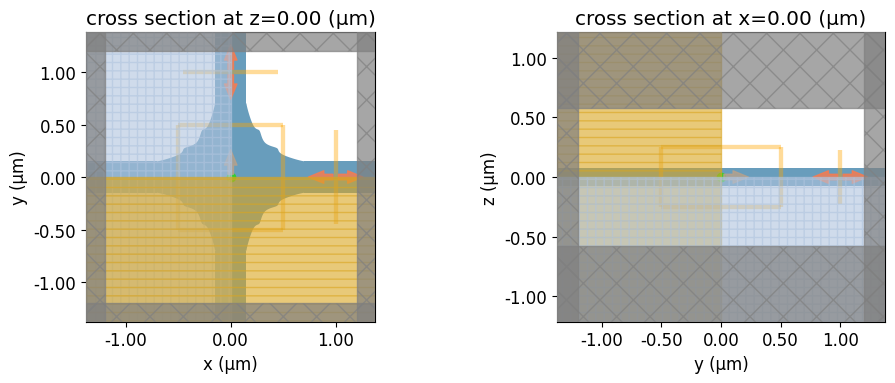
# Test it out
sim = make_sim(params=initial_params, use_fld_mnt=False)

fig, (ax1, ax2) = plt.subplots(1, 2, figsize=(10, 4), tight_layout=True)
sim.plot(z=0, ax=ax1)
sim.plot(x=0, ax=ax2)
plt.show()
Figures of Merit (FoMs)
The objective function will involve several figures of merit that quantify the optical performance of the device as well as a penalty that incentivizes designs that keep etched sidewalls more than 300 nm from the dipole.
For a dipole source, we are interested in:
- Purcell factor
- Coupling efficiency (into the desired output waveguide)
- Brightness (i.e., the product of the Purcell factor and coupling efficiency)
- Crosstalk (into modes in the orthogonal waveguide)`
def dipole_figs_of_merit(sim_data):
    # Sum the power flux out through the field monitor box at all frequencies monitored.
    dipole_power = anp.sum(
        anp.array(
            [anp.abs(sim_data[monitor.name].flux.values) for monitor in box_monitors]
        ),
        axis=0,
    )

    # Analytically calculate the power for a dipole in bulk semiconductor.
    # Must be increased when symmetry planes are used b/c image sources are used to enforce symmetry, which increases the
    # power effectively emitted by the dipole. Each symmetry plane doubles the number of sources, which doubles the amplitude.
    # The power is the square of amplitude, so the multiplication factor is 2^(2*num_sym_planes).
    sym_factor = 2 ** (2 * anp.sum(anp.abs(sim_data.simulation.symmetry)))
    bulk_power = (
        sym_factor
        * ((2 * anp.pi * freqs) ** 2 / (12 * anp.pi))
        * (td.MU_0 * n_AlGaAs / td.C_0)
    )

    # Purcell factor is the ratio of the two powers
    purcell = dipole_power / bulk_power
    # Coupling efficiency into the lowest mode of one output waveguide
    out_power = (
        anp.abs(sim_data["right_monitor"].amps.sel(direction="+", mode_index=0).values)
        ** 2
    )
    coupling = out_power / dipole_power
    # Brightness is the product of Purcell factor and coupling efficiency
    brightness = purcell * coupling
    # Crosstalk into one output waveguide (all modes)
    crosstalk_power = anp.sum(
        anp.array(
            [
                anp.abs(
                    sim_data["top_monitor"]
                    .amps.sel(direction="+", mode_index=idx)
                    .values
                )
                ** 2
                for idx in range(num_modes)
            ]
        ),
        axis=0,
    )
    crosstalk = crosstalk_power / dipole_power
    return purcell, coupling, brightness, crosstalk
Penalty: Border Distance
Quantum dots experience increased spectral diffusion and dephasing when they are too close to etched surfaces like those at the WGX border. Research indicates that borders <300 nm from the QD location increase the emission linewidth significantly. Thus, we want to keep the WGX border more than 300 nm from the dipole location. To incentivize this behavior in the optimization, we will use a penalty. The penalty below causes a nonlinear effective repulsion between border vertices and the location of the dipole at the origin.
def softplus(z):
    return anp.log1p(anp.exp(z))


def vertices_dist_penalty(vertices, border_d_min=0.300, curve_range=0.010, weight=1.0):
    """
    vertices: (M,2) np.array of vertex coordinates (x,y).
    border_d_min: float; minimum distance between the border and the dipole, in microns.
    curve_range: float; distance (in microns) around border_d_min over which the penalty transitions from zero to linear.
    weight: a weighting parameter
    """
    M = vertices.shape[0]
    z = (border_d_min - anp.linalg.norm(vertices, axis=1)) / curve_range
    P = weight * anp.sum(softplus(z))
    penalty = P / M  # Normalize by the number of vertices
    return penalty


def border_dist_penalty(params, border_d_min=0.300, curve_range=0.010, weight=1.0):
    vertices = make_vertices(params)
    return vertices_dist_penalty(vertices, border_d_min, curve_range, weight)
Optimization
Setup
DesignSpace
Tidy3D uses a DesignSpace object for gradient-free optimization approaches like Bayesian optimization, particle-swarm, and grid search.
# Bayesian optimization hyperparameters
initial_iter = 50  # To "prime" the Bayesian model
num_iter = 50  # number of iterations to refine the model
acq_func = "ucb"  # upper confidence bound, function used to choose next parameter set
kappa = 5.0  # higher means more exploration, lower means more exploitation. 5.0 is biased toward exploration.

# Parameters: (u1, v1, u2, v2, p),
#              Bounded 2-D coords for two free points and one point on the diagonal
span = (0, 1)  # The 2-D coords are normalized to this range.
# span2 = (0.001, 1) # The nominally different minimum prevents self-intersection during the cost-estimate, below.
d_span = (0, diag_max)
u1 = tdd.ParameterFloat(name="u1", span=span)
v1 = tdd.ParameterFloat(name="v1", span=span)
# u2 = tdd.ParameterFloat(name='u2', span=span2)
# v2 = tdd.ParameterFloat(name='v2', span=span2)
u2 = tdd.ParameterFloat(name="u2", span=span)
v2 = tdd.ParameterFloat(name="v2", span=span)
d = tdd.ParameterFloat(name="d", span=d_span)

# Assemble into a list to pass to tdd.DesignSpace
params = [u1, v1, u2, v2, d]

bayes_opt = tdd.MethodBayOpt(
    initial_iter=initial_iter, n_iter=num_iter, acq_func=acq_func, kappa=kappa
)

design_space = tdd.DesignSpace(
    method=bayes_opt,
    parameters=params,
    task_name="WGX_border_BayesOpt",
    path_dir="./data",
)

summary = design_space.summarize()
09:34:26 Eastern Daylight Time
                               Summary of DesignSpace

                               Method: MethodBayOpt
                               Method Args
                               initial_iter: 50
                               n_iter: 50
                               acq_func: ucb
                               kappa: 5.0
                               xi: 0.0

                               No. of Parameters: 5
                               Parameters: u1, v1, u2, v2, d
                               u1: ParameterFloat (0.0, 1.0)
                               v1: ParameterFloat (0.0, 1.0)
                               u2: ParameterFloat (0.0, 1.0)
                               v2: ParameterFloat (0.0, 1.0)
                               d: ParameterFloat (0.0, 0.5249999999999999)

                               Maximum Run Count: 100
History
It is good practice to store the history associated with an optimization for later analysis.
# Directory and file in which to store optimization history
WGX_BO_run_title = "wgx_border_bayesopt"
run_number = 20  # Change this to avoid overwriting previous data.
history_name = f"{WGX_BO_run_title}_{run_number:02d}.pkl"
history_dir = Path("misc")
history_dir.mkdir(parents=True, exist_ok=True)
history_file_1 = history_dir / history_name


# Helper functions to save and load the history
def save_history(history_dict: dict, history_file) -> None:
    """Convenience function to save the history to file."""
    with open(history_file, "wb") as file:
        pickle.dump(history_dict, file)


def load_history(history_file) -> dict:
    """Convenience method to load the history from file."""
    with open(history_file, "rb") as file:
        history_dict = pickle.load(file)
    return history_dict


history_dict_1 = dict()  # The history is blank for the moment.
Pre-function
The pre-function will receive arguments suggested by the optimizer and return a Simulation object.
def pre_func(**params):
    """Build a Simulation object from parameters suggested by the optimizer."""
    # Tidy's MethodBayOpt reorders the parameter alphabetically for some reason.
    param_array = [
        params["u1"],
        params["v1"],  # This avoids any reordering problems.
        params["u2"],
        params["v2"],
        params["d"],
    ]
    sim = make_sim(params=param_array, use_fld_mnt=False)
    # Store the parameters and the border distance penalty for later analysis.
    history_dict_1["params"].append(param_array.copy())
    history_dict_1["border_dist_pen"].append(border_dist_penalty(param_array))
    sim.attrs["param_array"] = param_array
    sim.attrs["border_dist_pen"] = border_dist_penalty(
        param_array
    )  # Stored here so post_func can access it later.
    return sim
Post-function and Objective Function
The DesignSpace runs the simulation returned by pre_func and gives the resulting sim_data object to the post_func. The post_func will then calculate the objective function value and any other auxiliary data. Thus, post_func serves the same general purpose as the objective function does in adjoint optimization. Furthermore, post_func returns the auxiliary data in a dictionary because it later gets converted to a dataframe.
# FoM weights
purcell_target = 1
weight_purcell = 0  # For a WGX alone, we don't want to encourage cavity-like designs.
weight_coupling = 1
weight_brightness = (
    0  # For a WGX alone, we don't want to encourage cavity-like designs.
)
weight_cross = (
    0  # The later adjoint optim will address the crosstalk, so use zero for now.
)

# Penalty weights
weight_border_dist = 0.1

# Brief description of the objective formula. Change it if you change the weights.
obj_descr = "coupling - border distance penalty, all weighted"


def post_func(sim_data: td.SimulationData) -> float:
    """Analyze SimulationData and return the objective value and auxiliary data."""

    purcell, coupling, brightness, crosstalk = dipole_figs_of_merit(sim_data)
    border_dist_pen = sim_data.simulation.attrs["border_dist_pen"]
    obj = (
        -((purcell_target - purcell[center_idx]) ** 2) * weight_purcell
        + coupling[center_idx] * weight_coupling
        + brightness[center_idx] * weight_brightness
        - crosstalk[center_idx] * weight_cross
        - weight_border_dist * border_dist_pen
    )

    # Save history
    history_dict_1["values"].append(obj)
    history_dict_1["crosstalk"].append(crosstalk)
    history_dict_1["purcell"].append(purcell)
    history_dict_1["coupling"].append(coupling)
    history_dict_1["brightness"].append(brightness)
    save_history(history_dict_1, history_file_1)

    return [
        obj,
        {
            "purcell": purcell,
            "coupling": coupling,
            "brightness": brightness,
            "crosstalk": crosstalk,
            "border_dist_pen": border_dist_pen,
        },
    ]
Metadata
It is good practice to store the metadata associated with an optimization to enable comparisons between multiple runs.
# Metadata associated with the optimization and simulation setup
WGX_BO_metadata = dict(
    # Source
    center_wavelength=wl,
    bandwidth=bw,
    # Material
    index=n_AlGaAs,
    wg_height=wg_height,
    wg_width=wg_width,
    # Waveguide crossing
    cross_width=cross_width,
    smidge=smidge,
    vertex_spacing=vertex_spacing,
    # Objective weights
    weight_purcell=weight_purcell,
    weight_coupling=weight_coupling,
    weight_brightness=weight_brightness,
    weight_cross=weight_cross,
    weight_border_dist=weight_border_dist,
    obj_descr=obj_descr,
    # BayesOpt hyperparameters
    initial_iter=initial_iter,
    num_iter=num_iter,
    acq_func=acq_func,
    kappa=kappa,
    pickle_file=history_name,
)
Check for a previous optimization and load it if it exists.
try:  # to load a previous optimization
    history_dict_1 = load_history(history_file_1)
    num_steps_completed = len(history_dict_1["values"])
    WGX_BO_metadata = history_dict_1["WGX_BO_metadata"]
    print("Loaded optimization checkpoint from file.")
    print(f"Found {num_steps_completed} iterations previously completed.")

except FileNotFoundError:  # Initialize a new optimization
    print("No previous checkpoint file found. Initializing a new optimization.")
    history_dict_1 = dict(
        values=[],
        purcell=[],
        coupling=[],
        brightness=[],
        crosstalk=[],
        border_dist_pen=[],
        params=[],
        WGX_BO_metadata=WGX_BO_metadata,
    )
No previous checkpoint file found. Initializing a new optimization.
Uncomment and run the cell below if there is an existing previous optimization but you don't want to load it.
# history_dict_1 = dict(
#         values = [],
#         purcell = [],
#         coupling = [],
#         brightness = [],
#         crosstalk = [],
#         border_dist_pen = [],
#         params = [],
#         WGX_BO_metadata = WGX_BO_metadata,
#     )
Estimated Cost
For tidy.DesignSpace objects, there is a helpful method that already exists to estimate the cost of a run.
cost_estimate = design_space.estimate_cost(
    pre_func
)  # Just uploads one job to get a cost estimate but doesn't run the job.
print(
    f"Estimated cost of BayesOpt using {initial_iter + num_iter} total simulations is {cost_estimate} flexcredits."
)
# Now we have to re-initialize the parameter and penalty history because pre_func added junk on this call.
history_dict_1["params"] = []
history_dict_1["border_dist_pen"] = []
09:34:30 Eastern Daylight Time Created task 'estimate_cost' with resource_id
                               'fdve-5e8a0eaa-8658-4491-a7c6-83800b425c9b' and
                               task_type 'FDTD'.
                               View task using web UI at
                               'https://tidy3d.simulation.cloud/workbench?taskId
                               =fdve-5e8a0eaa-8658-4491-a7c6-83800b425c9b'.
Task folder: 'default'.
Output()
09:34:36 Eastern Daylight Time Estimated FlexCredit cost: 0.025. Minimum cost
                               depends on task execution details. Use
                               'web.real_cost(task_id)' to get the billed
                               FlexCredit cost after a simulation run.
09:34:37 Eastern Daylight Time Estimated FlexCredit cost: 0.025. Minimum cost
                               depends on task execution details. Use
                               'web.real_cost(task_id)' to get the billed
                               FlexCredit cost after a simulation run.
Estimated cost of BayesOpt using 100 total simulations is 2.5 flexcredits.
Run the Optimization
# 50 initial simulations took about 10 minutes.
# 50 more iterations took about 2 hours.

td.config.logging_level = (
    "ERROR"  # Only give errors and ignore warnings to reduce clutter.
)

results = design_space.run(pre_func, post_func, verbose=True)

df = results.to_dataframe()
history_dict_1["df"] = df  # Add the dataframe of the results to the history...
save_history(history_dict_1, history_file_1)  # ...and save it.
09:34:40 Eastern Daylight Time Running 50 Simulations
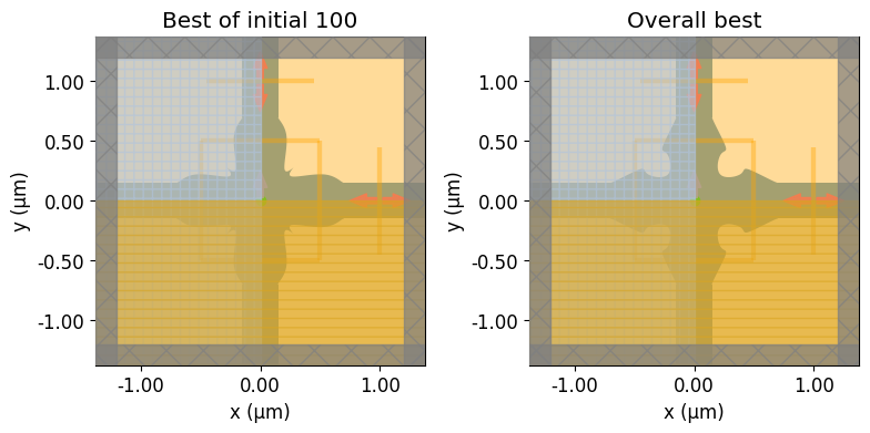
09:42:01 Eastern Daylight Time Best Fit from Initial Solutions: 0.366
09:42:02 Eastern Daylight Time Running 1 Simulations
09:44:01 Eastern Daylight Time Running 1 Simulations
09:47:46 Eastern Daylight Time Running 1 Simulations
09:49:50 Eastern Daylight Time Running 1 Simulations
09:52:37 Eastern Daylight Time Running 1 Simulations
09:55:33 Eastern Daylight Time Running 1 Simulations
09:58:27 Eastern Daylight Time Running 1 Simulations
10:00:46 Eastern Daylight Time Running 1 Simulations
10:03:37 Eastern Daylight Time Running 1 Simulations
10:06:34 Eastern Daylight Time Running 1 Simulations
10:09:25 Eastern Daylight Time Running 1 Simulations
10:12:53 Eastern Daylight Time Running 1 Simulations
10:15:15 Eastern Daylight Time Running 1 Simulations
10:17:39 Eastern Daylight Time Running 1 Simulations
10:20:15 Eastern Daylight Time Running 1 Simulations
10:23:04 Eastern Daylight Time Running 1 Simulations
10:25:22 Eastern Daylight Time Latest Best Fit on Iter 15: 0.368
Running 1 Simulations
10:28:10 Eastern Daylight Time Running 1 Simulations
10:30:01 Eastern Daylight Time Running 1 Simulations
10:32:37 Eastern Daylight Time Running 1 Simulations
10:35:14 Eastern Daylight Time Running 1 Simulations
10:39:15 Eastern Daylight Time Running 1 Simulations
10:41:51 Eastern Daylight Time Running 1 Simulations
10:44:11 Eastern Daylight Time Running 1 Simulations
10:46:40 Eastern Daylight Time Running 1 Simulations
10:50:42 Eastern Daylight Time Running 1 Simulations
10:53:15 Eastern Daylight Time Running 1 Simulations
10:56:10 Eastern Daylight Time Latest Best Fit on Iter 26: 0.376
10:56:11 Eastern Daylight Time Running 1 Simulations
10:58:34 Eastern Daylight Time Running 1 Simulations
11:01:25 Eastern Daylight Time Running 1 Simulations
11:04:52 Eastern Daylight Time Running 1 Simulations
11:07:57 Eastern Daylight Time Running 1 Simulations
11:10:31 Eastern Daylight Time Running 1 Simulations
11:14:15 Eastern Daylight Time Running 1 Simulations
11:16:41 Eastern Daylight Time Running 1 Simulations
11:20:04 Eastern Daylight Time Running 1 Simulations
11:21:57 Eastern Daylight Time Running 1 Simulations
11:25:02 Eastern Daylight Time Running 1 Simulations
11:27:14 Eastern Daylight Time Running 1 Simulations
11:29:14 Eastern Daylight Time Running 1 Simulations
11:31:38 Eastern Daylight Time Running 1 Simulations
11:33:56 Eastern Daylight Time Running 1 Simulations
11:34:37 Eastern Daylight Time Running 1 Simulations
11:36:38 Eastern Daylight Time Running 1 Simulations
11:37:47 Eastern Daylight Time Running 1 Simulations
11:38:43 Eastern Daylight Time Running 1 Simulations
11:39:39 Eastern Daylight Time Running 1 Simulations
11:40:22 Eastern Daylight Time Running 1 Simulations
11:41:01 Eastern Daylight Time Running 1 Simulations
11:41:45 Eastern Daylight Time Running 1 Simulations
11:42:34 Eastern Daylight Time Best Result: 0.3762434624587358
                               Best Parameters: d: 0.16293623904556734 u1:
                               0.4201964933386069 u2: 0.5426014917191861 v1:
                               0.27895228511879727 v2: 0.7775790739579105
results_dict = results.dict()
aux_values = results_dict[
    "aux_values"
]  # A tuple of dictionaries containing figures of merit.
Confirm Cost
# For a Bayesian optimization, num_tasks is:
num_tasks = initial_iter + num_iter

# Get the task information for the last num_tasks simulations.
task_dict_list = web.api.webapi.get_tasks(num_tasks)
cost_array = []
for task_dict in task_dict_list:
    cost_array.append(
        task_dict["realFlexUnit"]
    )  # The real cost is contained in the task dictionary
cost_array = anp.array(cost_array)
total_cost = anp.cumsum(cost_array)[-1]  # Sum the costs of all the simulations

# Might as well save the task information, too.
history_dict_1["task_dict_list"] = task_dict_list
save_history(history_dict_1, history_file_1)

print(f"Total cost of the optimization run: {total_cost:.4f} flexcredits")
print(f"Estimated cost: {cost_estimate:.3f} flexcredits")
print(f"Fraction of estimated cost: {total_cost / cost_estimate:.3f}")
Total cost of the optimization run: 2.5000 flexcredits
Estimated cost: 2.500 flexcredits
Fraction of estimated cost: 1.000
Analyzing WGX BO Results
After the optimization is finished, let's look at the results.
WGX BO Metadata
It's helpful to have the metadata printed out here for later reference.
history_dict_1["metadata"] = WGX_BO_metadata
WGX_BO_metadata
{'center_wavelength': 0.798,
 'bandwidth': 0.02,
 'index': np.float64(3.5693094750241627),
 'wg_height': 0.15,
 'wg_width': 0.3,
 'cross_width': 1.4,
 'smidge': 0.02,
 'vertex_spacing': 0.001,
 'weight_purcell': 0,
 'weight_coupling': 1,
 'weight_brightness': 0,
 'weight_cross': 0,
 'weight_border_dist': 0.1,
 'obj_descr': 'coupling - border distance penalty, all weighted',
 'initial_iter': 50,
 'num_iter': 50,
 'acq_func': 'ucb',
 'kappa': 5.0,
 'pickle_file': 'wgx_border_bayesopt_20.pkl'}
Sort by Objective Value
Sort everything by the best objective values.
df = history_dict_1["df"]
df_sorted = df.sort_values(by=["output"])
params = anp.array(history_dict_1["params"])
values = anp.array(history_dict_1["values"])
coupling = anp.array(history_dict_1["coupling"])
purcell = anp.array(history_dict_1["purcell"])
crosstalk = anp.array(history_dict_1["crosstalk"])
brightness = anp.array(history_dict_1["brightness"])
border_dist_pen = anp.array(history_dict_1["border_dist_pen"])

sort_idx = anp.argsort(values)
params_sorted = params[sort_idx, :]
values_sorted = values[sort_idx]
coupling_sorted = coupling[sort_idx]
purcell_sorted = purcell[sort_idx]
brightness_sorted = brightness[sort_idx]
crosstalk_sorted = crosstalk[sort_idx]
border_dist_pen_sorted = border_dist_pen[sort_idx]
Plot the nth-best design.
nth_best = 1
print(f"Objective: {values_sorted[-nth_best]:.5f}")
print(f"Purcell:   {purcell_sorted[-nth_best, center_idx]:.5f}")
print(f"Coupling:  {coupling_sorted[-nth_best, center_idx]:.5f}")
print(f"Crosstalk: {crosstalk_sorted[-nth_best, center_idx]:.5f}")
print(f"Penalty:   {border_dist_pen_sorted[-nth_best]:.5f}")
print(f"Parameters: {params_sorted[-nth_best, :]}")

test_sim = make_sim(params_sorted[-nth_best])
ax = test_sim.plot(z=0)
ax.set_title(f"{nth_best}th best design");
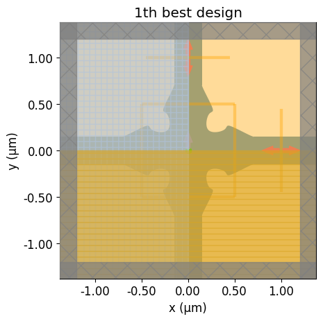
Objective: 0.37624
Purcell:   0.70399
Coupling:  0.37812
Crosstalk: 0.04473
Penalty:   0.01874
Parameters: [0.42019649 0.27895229 0.54260149 0.77757907 0.16293624]
best_BO_params_dict = results.optimizer.max["params"]
best_BO_params = [
    best_BO_params_dict["u1"],  # Doing this explicitly avoids any reordering problems.
    best_BO_params_dict["v1"],
    best_BO_params_dict["u2"],
    best_BO_params_dict["v2"],
    best_BO_params_dict["d"],
]
idx = -1
initial_best_dict = df[:initial_iter].sort_values(by=["output"]).iloc[idx].to_dict()
initial_param_array = [
    initial_best_dict["u1"],
    initial_best_dict["v1"],
    initial_best_dict["u2"],
    initial_best_dict["v2"],
    initial_best_dict["d"],
]

sim_initial_best = make_sim(initial_param_array)
sim_best = make_sim(best_BO_params)
fig, (ax1, ax2) = plt.subplots(1, 2, figsize=(8, 4), tight_layout=True)
ax1 = sim_initial_best.plot(z=0, ax=ax1)
ax1.set_title(f"Best of initial {initial_iter:d}")
ax2 = sim_best.plot(z=0, ax=ax2)
ax2.set_title("Overall best")
plt.show()
Plot the top five designs.
top_N = 5
param_array = df_sorted.to_numpy()[-top_N:, :-1][::-1]
obj_array = df_sorted.to_numpy()[-top_N:, -1][::-1]


# Helpful function to reorder the parameters because MethodBayesOpt
# puts them in alphabetical order, which is unhelpful.
def reorder_params(out_of_order_params):
    ordered_params = [
        out_of_order_params[1],  # u1
        out_of_order_params[3],  # v1
        out_of_order_params[2],  # u2
        out_of_order_params[4],  # v2
        out_of_order_params[0],
    ]  # d
    return anp.array(ordered_params)


# Plot from best to top_Nth best
fig, axs = plt.subplots(1, top_N, figsize=(10, 3), tight_layout=True)
for ax, top_params, obj in zip(axs, param_array, obj_array):
    sorted_params = reorder_params(top_params)
    cross_polyslab = make_polyslab(sorted_params)
    cross_polyslab.plot(z=0, ax=ax)
    ax.set_title(f"Obj={obj:.3f}")
    ax.set_xlabel(f"Penalty={border_dist_penalty(sorted_params):.5f}")
    ax.set_ylabel("")
    ax.set_xticklabels("")
    ax.set_yticklabels("")

print(f"Objective values: {df_sorted.to_numpy()[-top_N:, -1][::-1]}")
plt.show()
Objective values: [0.37624346 0.36838589 0.36586484 0.36566855 0.35357284]
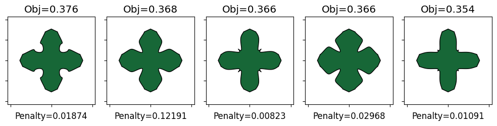
Let's also print the design parameters of the top designs. (Note that these parameters will be in alphabetical order.)
param_array
array([[0.16293624, 0.42019649, 0.54260149, 0.27895229, 0.77757907],
       [0.12224481, 0.64134311, 0.50510255, 0.63129037, 0.50575223],
       [0.33978088, 0.80394561, 0.01367886, 0.7329885 , 0.41697291],
       [0.12859768, 0.66970196, 0.54487972, 0.42848276, 0.42424459],
       [0.28667848, 0.69519754, 0.07560146, 0.80556661, 0.29881548]])
Figures of Merit Spectra
The best metric of the device performance is the spectral variation of the FoMs.
best_idx = anp.argmax(anp.array(results.values))
best_aux_values_1 = results.aux_values[best_idx]

fig, (ax1, ax2) = plt.subplots(1, 2, figsize=(8, 4), tight_layout=True)

ax1.plot(
    wl_range * 1000,
    anp.array(best_aux_values_1["purcell"]),
    ".-",
    label="Purcell factor",
)
ax1.plot(
    wl_range * 1000, anp.array(best_aux_values_1["coupling"]), ".-", label="Coupling"
)
ax1.legend()
ax1.set_xlabel("Wavelength (nm)")

ax2.plot(
    wl_range * 1000, anp.array(best_aux_values_1["crosstalk"]), ".-", label="Crosstalk"
)
ax2.set_xlabel("Wavelength (nm)")
ax2.legend()

print(f"Figures of merit at {wl * 1000:.0f} nm")
print(f"Purcell factor = {best_aux_values_1['purcell'][center_idx]}")
print(f"Coupling eff.  = {best_aux_values_1['coupling'][center_idx]}")
print(f"Brightness     = {best_aux_values_1['brightness'][center_idx]}")
print(f"Crosstalk      = {best_aux_values_1['crosstalk'][center_idx]}")

plt.show()
Figures of merit at 798 nm
Purcell factor = 0.7039918095204863
Coupling eff.  = 0.3781178262887307
Brightness     = 0.26619185274095647
Crosstalk      = 0.04472672123504394
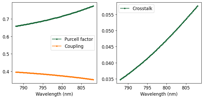
Recall that we want a high coupling efficiency and a low crosstalk at the design wavelength. A high Purcell factor is a secondary consideration but not directly incentivized by the objective function.
It appears that the BO design of the WGX produces a relatively high single-sided coupling efficiency of about 40%, while the crosstalk is around 4-5%. The efficiency and crosstalk could both be better, however, that improvement will occur in Stage 2: adjoint optimization of the WGX.
Fields in the Final Design
It is helpful to plot the electromagnetic fields themselves to visualize the device performance. Recall that the dipole source is oriented in the $y$-direction, so we plot the $y$-component of the electric field.
sim_best = make_sim(best_BO_params, use_fld_mnt=True)
sim_best_data = web.run(sim_best, task_name="wgx_border_BO_best", verbose=False)
f, ax = plt.subplots()
vminmax = 25000
sim_best_data.plot_field("field_xy", "Ey", ax=ax, vmin=-vminmax, vmax=vminmax)
ax.set_title("Best BO design")
plt.show()
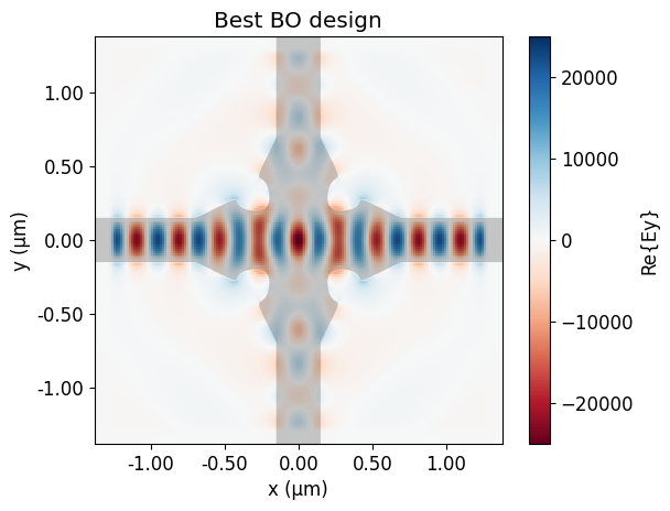
The emission mostly goes out the left and right waveguides, as desired. To a lesser extent, some emission goes out the top and bottom waveguides, which is the crosstalk. From the image, it looks like the crosstalk is mostly in a higher-order mode of the waveguides.
Directional Power Analysis
To determine where the emitted power goes when it doesn't go into the output waveguides we can use the box of monitors around the dipole.
# Taking the code from the figures of merit function, we can calculate the total power radiated by the dipole.
dipole_power = anp.sum(
    anp.array(
        [anp.abs(sim_best_data[monitor.name].flux.values) for monitor in box_monitors]
    ),
    axis=0,
)
# Its shape is (81,), which is one value for every frequency recorded in the simulation.

box_fluxes = anp.array(
    [anp.abs(sim_best_data[monitor.name].flux.values) for monitor in box_monitors]
)
side_names = ["Left", "Right", "Bottom", "Top", "Down", "Up"]
power_fractions = 100 * box_fluxes[:, center_idx] / dipole_power[center_idx]
print(f"Side\tPower fraction at {wl * 1000:.0f} nm (%)")
print("-------------------------")
for side, fraction in zip(side_names, power_fractions):
    if side == "Left" or side == "Right":
        print(
            f"{side}:\t{fraction:.2f}\t\tCoupling: {100 * best_aux_values_1['coupling'][center_idx]:.2f}\t\tDifference: {fraction - 100 * best_aux_values_1['coupling'][center_idx]:.2f}"
        )
    elif side == "Bottom" or side == "Top":
        print(
            f"{side}:\t{fraction:.2f}\t\tCrosstalk: {100 * best_aux_values_1['crosstalk'][center_idx]:.2f}\t\tDifference: {fraction - 100 * best_aux_values_1['crosstalk'][center_idx]:.2f}"
        )
    else:
        print(f"{side}:\t{fraction:.2f}")
Side	Power fraction at 798 nm (%)
-------------------------
Left:	39.12		Coupling: 37.81		Difference: 1.30
Right:	39.12		Coupling: 37.81		Difference: 1.30
Bottom:	7.16		Crosstalk: 4.47		Difference: 2.69
Top:	7.16		Crosstalk: 4.47		Difference: 2.69
Down:	3.72
Up:	3.72
The fractions of power exiting the six sides of the field monitor box around the dipole show where the lost emission is going. (Here "bottom" and "top" refer to the waveguides, while "down" and "up" refer to the directions out of the plane of the device.)
Comparison: Best BO Design vs. Plain Waveguide Crossing
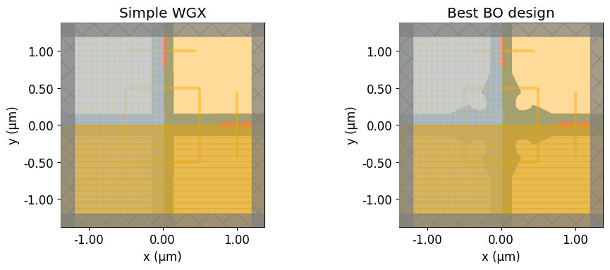
We can compare the Bayesian-optimized design with a simple waveguide crossing. We will set use_fld_mnt = True so we can visualize the field distributions of the designs.
params_simpleWGX = [
    0.0,
    0.0,
    0.0,
    0.0,
    wg_width / 2,
]  # parameters for a simple waveguide crossing
sim_simpleWGX = make_sim(params_simpleWGX, use_fld_mnt=True)

fig, (ax1, ax2) = plt.subplots(1, 2, figsize=(10, 4), tight_layout=True)
sim_simpleWGX.plot(z=0, ax=ax1)
ax1.set_title("Simple WGX")
sim_best.plot(z=0, ax=ax2)
ax2.set_title("Best BO design")
plt.show()
simpleWGX_sim_data = web.run(sim_simpleWGX, task_name="wgx_simple", verbose=False)
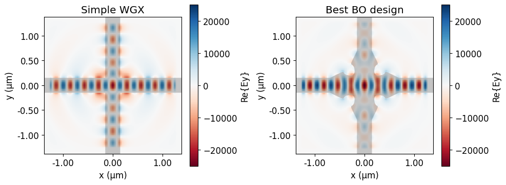
Plot the field distributions.
f, (ax1, ax2) = plt.subplots(1, 2, tight_layout=True, figsize=(10, 4))
vminmax = 25000

_ = simpleWGX_sim_data.plot_field("field_xy", "Ey", ax=ax1, vmin=-vminmax, vmax=vminmax)
ax1.set_title("Simple WGX")

_ = sim_best_data.plot_field("field_xy", "Ey", ax=ax2, vmin=-vminmax, vmax=vminmax)
ax2.set_title("Best BO design")

plt.show()
simple_purcell, simple_coupling, simple_brightness, simple_crosstalk = (
    dipole_figs_of_merit(simpleWGX_sim_data)
)

print(f"Figures of merit at {wl * 1000:.0f} n\n")

print("Simple WGX")
print(f"\tPurcell factor = {simple_purcell[center_idx]:.3f}")
print(f"\tCoupling eff.  = {simple_coupling[center_idx]:.3f}")
print(f"\tBrightness     = {simple_brightness[center_idx]:.3f}")
print(f"\tCrosstalk      = {simple_crosstalk[center_idx]:.4f}")
print()

print("BO design")
print(f"\tPurcell factor = {best_aux_values_1['purcell'][center_idx]:.3f}")
print(f"\tCoupling eff.  = {best_aux_values_1['coupling'][center_idx]:.3f}")
print(f"\tBrightness     = {best_aux_values_1['brightness'][center_idx]:.3f}")
print(f"\tCrosstalk      = {best_aux_values_1['crosstalk'][center_idx]:.4f}")
Figures of merit at 798 n

Simple WGX
	Purcell factor = 0.599
	Coupling eff.  = 0.306
	Brightness     = 0.183
	Crosstalk      = 0.1076

BO design
	Purcell factor = 0.704
	Coupling eff.  = 0.378
	Brightness     = 0.266
	Crosstalk      = 0.0447
Compared to a simple WGX, the BO WGX design has increased coupling efficiency to the desired waveguides (38% to 31%) and less than half the crosstalk in the undesired waveguides (4.5% to 11%). That's a big improvement even for just the first Stage of the optimization, where the crosstalk was not even included in the objective function.
Stage 2: Adjoint Optimization of WGX
Starting with the results of the initial, low-dimensional parameterization of the WGX border, we will use adjoint optimization to increase the coupling efficiency and decrease the crosstalk while maintaining a dipole-to-border distance greater than 300 nm. We can use any parameter set from the low-dimensional parameterization of the border used in Stage 1. The border will be resampled to find initial control points for a spline representation.
This section of the notebook will cost approximately 1.25 flexcredits and take about 5.5 hours to run.Re-parameterization for Adjoint Optimization
We will re-parameterize the device border for use in adjoint optimization by densely sampling the quarter-border, then taking 30 points spaced approximately equally along the arc of the curve to be control points for a natural cubic spline (an interpolating spline). This time we will use the built-in function tidy3d.plugins.autograd.interpolate_spline.
num_free_pts = 30
num_vertices = 600  # along one quarter of the device border

# Get the control points and vertices of the quarter border from the best Stage 1 parameters
BO_ctrl_pts = ctrl_pt_array_from_params(
    best_BO_params, inner_corner, outer_corner, wg_corner1
)
quarter_border_vertices = make_border_vertices(basis_funcs, BO_ctrl_pts)
N_vertices = len(quarter_border_vertices)
midpoint = int(N_vertices / 2)

# Cut off the vertices that are to the right of the "smidge" point.
# This ensures that the eventual interpolating spline inserts correctly into the waveguide.
cut_border = quarter_border_vertices[
    [vertex[0] < wg_corner2[0] for vertex in quarter_border_vertices]
]
N_vertices_2 = len(cut_border)
midpoint_2 = int(midpoint - (N_vertices - N_vertices_2))

# Sample equidistant along the border rather than equally spaced in the spline parameter.
inter_point_differences = anp.diff(cut_border[: midpoint_2 + 1], axis=0)
inter_point_distances = anp.linalg.norm(inter_point_differences, axis=-1)
cumulative_distance = anp.cumsum(inter_point_distances)
cumulative_distance /= cumulative_distance[-1]  # Normalize the cumulative distance
cumulative_distance = anp.concatenate(
    ([0.0], cumulative_distance)
)  # Add zero cumulative distance to make the first point.

new_ctrl_pts = cut_border[1 : midpoint_2 + 1][
    1 == anp.diff(cumulative_distance * (num_free_pts + 1) // 1)
]


def make_reparam_border_vertices(control_points, num_vertices=600):
    """
    Returns the vertices for the upper-right border of the waveguide cross.
    """
    N_ctrl = len(control_points)
    x_ctrl = control_points[:, 0]
    y_ctrl = control_points[:, 1]
    t_ctrl = anp.linspace(0.0, 1.0, N_ctrl)
    t_eval, x_eval = interpolate_spline(
        t_ctrl, x_ctrl, order=3, num_points=num_vertices
    )
    t_eval, y_eval = interpolate_spline(
        t_ctrl, y_ctrl, order=3, num_points=num_vertices
    )
    return anp.stack([x_eval, y_eval], axis=-1)


def make_params_from(control_points):
    """
    Take the control points sampled from the initial design and make the parameter array that would reproduce them.
    """
    num_free_pts = len(control_points) - 1
    assert isinstance(num_free_pts, int), "Length of control_points must be odd."
    params = control_points.flatten()[
        :-1
    ]  # All in one line, dropping the duplicated diagonal point dimension.
    return params


def make_control_points_from(params, smidge=0.020):
    """
    params (NDarray): 2*num_control_pts+1 design parameters that are the (x,y) positions of the free control points
    plus the y=x position of the middle control point along the diagonal.
    smidge (float): X-distance between the fixed control point on the corner of the waveguide and the fixed neighboring point.

    Returns the control points for the upper-right quarter of the WGX border.
    """

    # Fixed points at and near the waveguide corner
    p_corner = anp.array([[cross_width / 2, wg_width / 2]])
    p_2 = p_corner - anp.array([[smidge, 0]])

    # Point along the diagonal
    p_mid = anp.array([[params[-1], params[-1]]])

    # Free points between the corner and the diagonal
    p_others = params[:-1].reshape([-1, 2])

    control_points = anp.concatenate((p_corner, p_2, p_others, p_mid))
    mirrored_points = control_points[-2::-1, ::-1]
    control_points = anp.concatenate((control_points, mirrored_points))
    return control_points


def make_reparam_vertices(params):
    ctrl_pts = make_control_points_from(params, smidge=smidge)
    quarter_border_vertices = make_reparam_border_vertices(
        ctrl_pts, num_vertices=num_vertices
    )
    vertices = border_vertices_to_all(quarter_border_vertices)
    return vertices


# Helper functions for reparameterized border
def make_reparam_polyslab(params: anp.ndarray) -> td.PolySlab:
    """Make a `tidy3d.PolySlab` for the device given the design parameters."""
    vertices = make_reparam_vertices(params)
    return td.PolySlab(
        vertices=vertices, slab_bounds=(-wg_height / 2, wg_height / 2), axis=2
    )


def make_reparam_structure(params) -> td.Structure:
    cross_polyslab = make_reparam_polyslab(params)
    return td.Structure(geometry=cross_polyslab, medium=AlGaAs_simple)


reparams = make_params_from(new_ctrl_pts)
assert reparams.shape == (2 * num_free_pts + 1,)

cross_polyslab_2 = make_reparam_polyslab(reparams)
ax = cross_polyslab_2.plot(z=0)
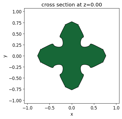
The reparameterization works. Now make_reparam_structure can be used in a new make_sim function for adjoint optimization.
make_sim Function
def make_sim(
    params,
    use_fld_mnt: bool = True,
) -> td.Simulation:
    # Structures
    cross_struct = make_reparam_structure(params)
    structures = static_structures + [cross_struct]

    # Sources and monitors:
    sources = [dipole_src]
    monitors = [right_monitor, top_monitor] + box_monitors

    if use_fld_mnt == True:
        monitors = monitors + [field_monitor_xy]

    # Simulation size is the bounding box of the geometry modified by some multiple of pml_spacing.
    pml_spacing = 0.5
    sim_size = (
        2 * wg_length / 3 + cross_width - 1 * pml_spacing,
        2 * wg_length / 3 + cross_width - 1 * pml_spacing,
        wg_height + 2 * pml_spacing,
    )

    # Initialize simulation
    sim = td.Simulation(
        structures=structures,
        sources=sources,
        monitors=monitors,
        size=sim_size,
        center=origin,
        grid_spec=grid_spec,
        run_time=run_time,
        boundary_spec=boundary_spec,
        symmetry=symmetry_A,
    )
    return sim


sim = make_sim(params=reparams, use_fld_mnt=False)

fig, (ax1, ax2) = plt.subplots(1, 2, figsize=(10, 4), tight_layout=True)
sim.plot(z=0, ax=ax1)
sim.plot(x=0, ax=ax2)
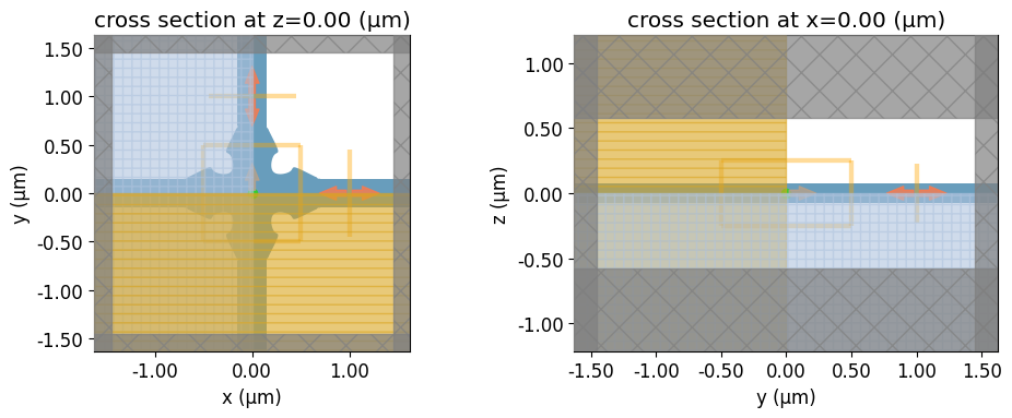
plt.show()
Penalties
In addition to the border distance penalty used above, we require additional penalties for the new parameterization.
Curvature Penalty
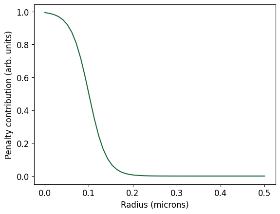
With a cubic spline parameterization, it is possible to generate structures with wildly varying radii of curvature which may be difficult to fabricate. To alleviate this, we introduce a minimum radius of curvature penalty transformation using the tidy3d autograd utilities. The penalty will take a set of vertices, compute the local radius of curvature using a quadratic Bezier curve, and return an average penalty function that depends on how much smaller the local radii are compared to a desired minimum radius.
min_curv_radius = 0.100  # microns
alpha = 1.0  # a weight parameter
kappa = 50.0  # Tidy suggests kappa = 10.0 as the default argument, but 50 works better in this case.
curve_penalty = make_curvature_penalty(
    min_radius=min_curv_radius, alpha=alpha, kappa=kappa
)
# The kappa parameter determines the sharpness of the logistic function step from zero to one.
# A higher value of kappa means that the smallest radii of curvature contribute more to the penalty
# compared to larger radii of curvature. The alpha parameter is simply an overall weight.
Here is an illustration of the sigmoid shape of the local curvature penalty that gets averaged over the whole border curve.
sigmoid = lambda r: 1 / (anp.exp(kappa * (r - min_curv_radius)) + 1)
r = anp.linspace(0, 0.5, 50)
plt.plot(r, sigmoid(r), "-")
plt.xlabel("Radius (microns)")
plt.ylabel("Penalty contribution (arb. units)")
plt.show()
Minimum Vertex Separation Penalty
The purpose of this penalty is to avoid self-intersection of the border. It causes a nonlinear effective repulsion between non-adjacent vertices that form the border. It doesn't act directly on the control points, but it does affect them indirectly via back-propagation through the spline relationship between vertices and control points.
def softplus(z):
    # softplus(z) ~ max(0, z) but smooth and differentiable
    return anp.log1p(anp.exp(z))


def min_separation_penalty(vertices, vert_d_min=1e-2, alpha=1.0, eps=1e-3, skip=2):
    """
    vertices: (M,2) np.array of vertex coordinates (x,y).
    vert_d_min: threshold distance between vertices where the penalty is at half-maximum.
    alpha: a weighting parameter
    eps: microns, a distance over which the penalty climbs from low to high; controls "sharpness" of the penalty.
    skip: number of immediate neighboring vertices to skip when calculating the penalty for a given vertex.
    """
    M = vertices.shape[0]
    P = 0.0
    for i in range(M):
        dif = vertices[i + skip :] - vertices[i]  # skip some immediate neighbors
        d = anp.sqrt(anp.sum(dif * dif, axis=1))
        z = (vert_d_min - d) / eps
        P = P + alpha * anp.sum(softplus(z))
    return P / M  # penalty normalized by the number of vertices/points
Control-Space Smoothness Penalty
The purpose of this penalty, like the curvature penalty above, is to incentivize the optimization to produce border splines that are not too curved. However, this penalty works directly on the control points rather than through the vertices of the interpolating spline. It is a scalar "smoothness" penalty based on the angles of the polygonal chain formed by the control points. This includes the two fixed points at the corner of the output waveguide, the num_free_pts free control points along 1/8th of the border, the mid-point on the diagonal, and the last free control point mirrored across the diagonal.
def control_space_smoothness(params, eps=1e-12):
    """
    params: 1D array of design parameters.
        params[:-1] reshape to (N,2) free control points.
        params[-1]  scalar d for diagonal apex (d,d).

    Returns:
        Scalar smoothness penalty based on turning angles
        of the full polygonal chain including:
            fixed0 → fixed1 → free points → apex → mirrored last free point
    """

    # Fixed points at and near the waveguide corner
    p_corner = anp.array([[cross_width / 2, wg_width / 2]])
    p_2 = p_corner - anp.array([[smidge, 0]])

    # Free control points
    ctrl_free = params[:-1].reshape((-1, 2))  # (N,2)
    N = ctrl_free.shape[0]

    # Diagonal apex
    d = params[-1]
    apex = anp.array([[d, d]])  # (1,2)

    # Mirror the last free control point across x=y
    last = ctrl_free[-1]
    mirrored = anp.array([[last[1], last[0]]])  # (1,2)

    # Build full chain
    points = [
        p_corner,  # (1,2)
        p_2,  # (1,2)
        ctrl_free,  # (N,2)
        apex,  # (1,2)
        mirrored,  # (1,2)
    ]

    ctrl = anp.concatenate(points, axis=0)  # (M,2)
    M = ctrl.shape[0]

    if M < 3:
        return anp.array(0.0)

    # Segments
    seg = ctrl[1:] - ctrl[:-1]  # (M-1,2)
    seg_len = anp.sqrt(anp.sum(seg**2, axis=1)) + eps
    u = seg / seg_len[:, None]  # unit directions

    # Turning angles via dot products
    dot = anp.sum(u[1:] * u[:-1], axis=1)  # (M-2,)
    dot = anp.clip(dot, -1.0, 1.0)

    # Bending measure
    bending = 1.0 - dot  # ~theta^2/2 for small angles
    penalty = anp.sum(bending**2)

    return penalty
Control Point Spacing Penalty
This penalty prevents the control points from getting too close to each other. Without this penalty and an appropriate choice of minimum control-point spacing, the control points tend to "bunch up" into pairs during the adjoint optimization.
def control_point_spacing_penalty(params, ctrl_s_min=0.005, eps=1e-12):
    """
    Penalize neighboring control points getting too close.

    params: 1D array of design parameters.
        params[:-1] -> (N,2) free control points.
        params[-1]  -> scalar d for apex (d,d).

    ctrl_s_min: float
        Desired minimum spacing between control points (in microns).

    eps: float
        Small amount to avoid a divide-by-zero error

    Returns:
        Scalar spacing penalty. Large when some segments are shorter than ctrl_s_min.
    """

    # Fixed points at and near the waveguide corner
    p_corner = anp.array([[cross_width / 2, wg_width / 2]])
    p_2 = p_corner - anp.array([[smidge, 0]])

    # Free control points
    ctrl_free = params[:-1].reshape((-1, 2))  # (N,2)
    d = params[-1]
    apex = anp.array([[d, d]])  # (1,2)

    # Mirror last free control point across x = y
    last = ctrl_free[-1]
    mirrored = anp.array([[last[1], last[0]]])  # (1,2)

    # Full chain (same as smoothness)
    points = [
        p_corner,  # (1,2)
        p_2,  # (1,2)
        ctrl_free,  # (N,2)
        apex,  # (1,2)
        mirrored,  # (1,2)
    ]
    ctrl = anp.concatenate(points, axis=0)  # (M,2)

    # Segment lengths
    seg = ctrl[1:] - ctrl[:-1]  # (M-1,2)
    seg_len = anp.sqrt(anp.sum(seg**2, axis=1)) + eps  # (M-1,)

    z = (ctrl_s_min - seg_len) / (ctrl_s_min + eps)  # dimensionless
    # Only positive z (seg_len < ctrl_s_min) contribute significantly
    penalty = anp.sum(softplus(z) ** 2)

    return penalty
Penalty Wrapper Function
For Stage 2, we can define a penalty wrapper function to use the new functions that take the parameters and make the control points and vertices. We wrap the penalties to look at only the upper-right quadrant of the cross because the others are the same by symmetry.
# Vertex separation penalty
alpha = 1.0
vert_d_min = 0.025  # microns
eps = 1e-3  # microns
skip = (
    num_vertices // num_free_pts
)  # scale the number skipped to the number of vertices per interval

# Control point spacing penalty
ctrl_s_min = 0.010  # Initial ctrl pt spacing is about 0.014; this should be just a bit below that value.

# Border distance penalty
border_d_min = (
    0.300  # This is the 300-nm minimum distance from the border to the dipole.
)
curve_range = 0.010


def eval_penalties(params):
    """Evaluate all the penalties on a set of params."""
    control_points = make_control_points_from(params)
    border_vertices = make_reparam_border_vertices(control_points)

    curve_pen = curve_penalty(border_vertices)
    min_sep_pen = min_separation_penalty(
        border_vertices, vert_d_min=vert_d_min, alpha=alpha, eps=eps, skip=skip
    )

    smoothness_pen = control_space_smoothness(params)

    spacing_pen = control_point_spacing_penalty(params, ctrl_s_min)

    border_dist_pen = vertices_dist_penalty(border_vertices, border_d_min, curve_range)

    return (curve_pen, min_sep_pen, smoothness_pen, spacing_pen, border_dist_pen)


# Penalties for the initial reparameterized design.
eval_penalties(reparams)
(np.float64(0.2754338954673494),
 np.float64(7.046104849395304e-05),
 np.float64(0.13858456302808056),
 np.float64(5.636927791842889),
 np.float64(0.018531546603880143))
Objective Definition
Now we can define our objective function to maximize. The objective function first generates a simulation given the parameters, runs the simulation using the built-in web.run() function, calculates the figures of merit and penalties, and calculates the weighted objective function:
$ - w_P ( F_P^{(target)} - F_P )^2 + w_\eta \eta +w_B F_P \eta - w_x \eta_x - w_{pen} \cdot P $
Here, $F_P$ is the Purcell factor, $\eta$ is the coupling efficiency, $\eta_x$ is the crosstalk, $P$ is the array of penalties, and the $w_j$ are the corresponding weights.
Note that in this stage we want to strongly disincentivize crosstalk, so we increase the crosstalk weight in the objective function from zero (as in Stage 1) to 5.
# We can make a variable that `objective` can modify in place even when called inside `value_and_grad`.
# Then we can access that after running `value_and_grad`
sim_data_last = [None]

# Brief description of the objective formula to store as metadata.
obj_descr = "coupling - crosstalk - five penalties, no Purcell included"

# Weights for dipole source. CHANGE THE obj_descr IF YOU CHANGE THE WEIGHTS.
purcell_target = 1
weight_purcell = 0  # For a WGX alone, we don't want to encourage cavity-like designs.
weight_coupling = 1
weight_brightness = (
    0  # For a WGX alone, we don't want to encourage cavity-like designs.
)
weight_cross = 5  # In this stage we want to strongly disincentivize crosstalk.

# Weights for penalties. CHANGE THE obj_descr IF YOU CHANGE THE WEIGHTS.
weight_curve_pen = 0.01
weight_minsep_pen = 0.3
weight_smooth = 0.03
weight_spacing = 0.01
weight_border_dist = 0.01


def objective(
    params: anp.ndarray, use_fld_mnt: bool = False, verbose: bool = False
) -> float:

    sim = make_sim(params=params, use_fld_mnt=use_fld_mnt)
    sim_data = web.run(sim, task_name="wgx_border_adjoint", verbose=verbose)
    sim_data_last[0] = sim_data

    purcell, coupling, brightness, crosstalk = dipole_figs_of_merit(sim_data)
    curve_pen, min_sep_pen, smoothness_pen, spacing_pen, border_dist_pen = (
        eval_penalties(params)
    )
    obj = (
        -((purcell_target - purcell[center_idx]) ** 2) * weight_purcell
        + coupling[center_idx] * weight_coupling
        + brightness[center_idx] * weight_brightness
        - crosstalk[center_idx] * weight_cross
        - curve_pen * weight_curve_pen
        - min_sep_pen * weight_minsep_pen
        - smoothness_pen * weight_smooth
        - spacing_pen * weight_spacing
        - weight_border_dist * border_dist_pen
    )
    return obj, [
        purcell,
        coupling,
        brightness,
        crosstalk,
        curve_pen,
        min_sep_pen,
        smoothness_pen,
        spacing_pen,
        border_dist_pen,
    ]


min_or_max = -1  # 1=minimize the objective; -1=maximize the objective
Optional Tests
We can test out the calculation of the objective function and figures of merit.
obj, foms = objective(params=reparams, use_fld_mnt=True, verbose=True)
# Took 1:22 mins and cost 0.025 flexcredits.
11:48:20 Eastern Daylight Time Created task 'wgx_border_adjoint' with
                               resource_id
                               'fdve-578c1358-25d8-40f3-9b9c-6302ce25d373' and
                               task_type 'FDTD'.
                               View task using web UI at
                               'https://tidy3d.simulation.cloud/workbench?taskId
                               =fdve-578c1358-25d8-40f3-9b9c-6302ce25d373'.
Task folder: 'default'.
Output()
11:48:26 Eastern Daylight Time Estimated FlexCredit cost: 0.025. Minimum cost
                               depends on task execution details. Use
                               'web.real_cost(task_id)' to get the billed
                               FlexCredit cost after a simulation run.
11:48:27 Eastern Daylight Time status = queued
                               To cancel the simulation, use
                               'web.abort(task_id)' or 'web.delete(task_id)' or
                               abort/delete the task in the web UI. Terminating
                               the Python script will not stop the job running
                               on the cloud.
Output()
11:48:39 Eastern Daylight Time starting up solver
11:48:40 Eastern Daylight Time running solver
Output()
11:48:43 Eastern Daylight Time early shutoff detected at 60%, exiting.
status = postprocess
Output()
11:48:51 Eastern Daylight Time status = success
11:48:53 Eastern Daylight Time View simulation result at
                               'https://tidy3d.simulation.cloud/workbench?taskId
                               =fdve-578c1358-25d8-40f3-9b9c-6302ce25d373'.
Output()
11:49:07 Eastern Daylight Time Loading simulation from simulation_data.hdf5
We can obtain the auxiliary output (i.e., the individual figures of merit and penalties) from the output of objective like this.
(
    purcell,
    coupling,
    brightness,
    crosstalk,
    curve_pen,
    min_sep_pen,
    smoothness_pen,
    spacing_pen,
    border_dist_pen,
) = [out for out in foms]
print(f"Objective value = {obj:.3f}")
print(f"FoMs at {wl * 1000:.0f} nm:")
print(f"\tPurcell = {purcell[center_idx]:.3f}")
print(f"\tCoupling (one-sided) = {coupling[center_idx]:.3f}")
print(f"\tBrightness (one-sided) = {brightness[center_idx]:.3f}")
print(f"\tCrosstalk (one-sided) = {crosstalk[center_idx]:.3f}")
print("Penalties:")
print(f"\tCurvature Penalty = {curve_pen:.3f}")
print(f"\tMinimum Separation Penalty = {min_sep_pen:.3f}")
print(f"\tSmoothness Penalty = {smoothness_pen:.3f}")
print(f"\tSpacing Penalty = {spacing_pen:.3f}")
print(f"\tBorder Distance Penalty = {border_dist_pen:.3f}")
Objective value = 0.083
FoMs at 798 nm:
	Purcell = 0.710
	Coupling (one-sided) = 0.375
	Brightness (one-sided) = 0.266
	Crosstalk (one-sided) = 0.046
Penalties:
	Curvature Penalty = 0.275
	Minimum Separation Penalty = 0.000
	Smoothness Penalty = 0.139
	Spacing Penalty = 5.637
	Border Distance Penalty = 0.019
Adjoint Gradient
The critical part of the adjoint approach is to calculate the gradient of the objective function with respect to the design parameters. The function tidy3d.plugins.autograd.value_and_grad automates this process.
val_grad = value_and_grad(objective, has_aux=True)
# Calling value_and_grad with has_aux=True enables passing additional
# arguments to the objective beyond the design parameters.
Optional Tests
Let's run this function and take a look at the outputs.
# This takes about 5 minutes to run.
(val, grad), foms = val_grad(reparams, use_fld_mnt=False, verbose=True)
11:49:24 Eastern Daylight Time Created task 'wgx_border_adjoint' with
                               resource_id
                               'fdve-74ee59fd-38ba-4a5c-803b-b6e310df1476' and
                               task_type 'FDTD'.
                               View task using web UI at
                               'https://tidy3d.simulation.cloud/workbench?taskId
                               =fdve-74ee59fd-38ba-4a5c-803b-b6e310df1476'.
Task folder: 'default'.
Output()
11:49:29 Eastern Daylight Time Estimated FlexCredit cost: 0.025. Minimum cost
                               depends on task execution details. Use
                               'web.real_cost(task_id)' to get the billed
                               FlexCredit cost after a simulation run.
Output()
11:49:34 Eastern Daylight Time status = queued
                               To cancel the simulation, use
                               'web.abort(task_id)' or 'web.delete(task_id)' or
                               abort/delete the task in the web UI. Terminating
                               the Python script will not stop the job running
                               on the cloud.
Output()
11:49:44 Eastern Daylight Time starting up solver
11:49:45 Eastern Daylight Time running solver
Output()
11:49:49 Eastern Daylight Time early shutoff detected at 60%, exiting.
status = postprocess
Output()
11:49:59 Eastern Daylight Time status = success
11:50:01 Eastern Daylight Time View simulation result at
                               'https://tidy3d.simulation.cloud/workbench?taskId
                               =fdve-74ee59fd-38ba-4a5c-803b-b6e310df1476'.
Output()
11:50:14 Eastern Daylight Time Loading simulation from
                               simulation_data_adjoint.hdf5
11:53:53 Eastern Daylight Time Started working on Batch containing 1 tasks.
11:54:04 Eastern Daylight Time Maximum FlexCredit cost: 0.025 for the whole
                               batch.
                               Use 'Batch.real_cost()' to get the billed
                               FlexCredit cost after completion.
Output()
11:54:35 Eastern Daylight Time Batch complete.
Output()
We have access to the objective value and its gradient w.r.t. the design parameters.
print(val)
print(grad)
0.08288614499531723
[ 1.06567484e+00  1.02150858e+00  4.59558132e-01  1.27250846e+00
  6.70059346e-01  1.25075249e+00  6.65102401e-01  1.42759369e+00
  6.64837626e-01  1.17969493e+00  5.73113626e-01  1.35169953e+00
  6.12100232e-01  1.04291989e+00  4.64086017e-01  1.10011732e+00
  4.42169396e-01  8.56650648e-01  4.12233543e-01  7.84495297e-01
  2.71512030e-01  4.71393838e-01  1.14649339e-01  4.43466259e-01
  2.06493457e-01  2.31682513e-01 -6.69720466e-04  2.05583639e-01
  1.96295168e-02 -1.82387332e-02 -1.24674311e-01  3.98453801e-01
  6.69477204e-01 -1.04405493e+00 -1.24894112e-01  1.89614617e-01
  5.60637023e-01 -4.78974819e-01  7.84792023e-01 -1.01077338e+00
  3.82960341e-01 -8.72975824e-01  5.03373815e-01 -1.28635718e+00
  1.60641870e-01 -5.18634361e-01 -1.91759498e-01  8.56079462e-01
 -1.85537553e-01  1.46936759e+00 -7.22770100e-02  2.04875675e+00
  1.14134615e-01  2.63755102e+00  5.79319760e-01  3.17249683e+00
  1.58759581e+00  4.64760271e+00  3.00470450e+00  4.51500002e+00
  4.02029292e+00]
We can access the most recent simulation data run by the objective function as follows.
sim_data_last[0].simulation.plot(z=0);
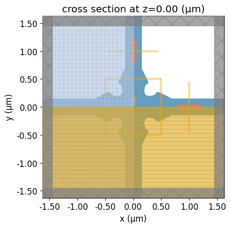
Hyperparameters, Metadata, and History
# Hyperparameters for optimization routine
num_steps = 50
learning_rate = 0.005

# Initialize adam optimizer with the starting parameters
optimizer = optax.adam(learning_rate=learning_rate)
opt_state = optimizer.init(reparams)

# Directory and file in which to store optimization history
WGX_adoint_run_title = "wgx_border_adjoint"
history_name = f"{WGX_adoint_run_title}_{run_number:02d}.pkl"
history_dir = Path("misc")
history_dir.mkdir(parents=True, exist_ok=True)
history_file_2 = history_dir / history_name

# Metadata associated with the optimization and simulation setup
WGX_adjoint_metadata = dict(
    # Source
    center_wavelength=wl,
    bandwidth=bw,
    # Material
    index=n_AlGaAs,
    wg_height=wg_height,
    wg_width=wg_width,
    # Waveguide crossing
    cross_width=cross_width,
    smidge=smidge,
    num_free_pts=num_free_pts,
    num_vertices=num_vertices,
    low_d_params=best_BO_params,
    # Penalty parameters
    min_curv_radius=min_curv_radius,
    penalty_alpha=alpha,
    penalty_kappa=kappa,
    min_vertex_sep=vert_d_min,
    penalty_eps=eps,
    skip=skip,
    ctrl_s_min=ctrl_s_min,
    border_d_min=border_d_min,
    curve_range=curve_range,
    # Objective weights
    obj_descr=obj_descr,
    weight_purcell=weight_purcell,
    weight_coupling=weight_coupling,
    weight_brightness=weight_brightness,
    weight_cross=weight_cross,
    weight_curve_pen=weight_curve_pen,
    weight_minsep_pen=weight_minsep_pen,
    weight_smooth=weight_smooth,
    weight_spacing=weight_spacing,
    weight_border_dist=weight_border_dist,
    # Optimizer hyperparameters
    num_steps=num_steps,
    learning_rate=learning_rate,
    pickle_file=history_name,
)
Check for a previous optimization and load it if it exists.
try:  # to load a previous optimization
    history_dict_2 = load_history(history_file_2)
    opt_state = history_dict_2["opt_states"][-1]
    params = history_dict_2["params"][-1].copy()
    num_steps_completed = len(history_dict_2["values"])
    WGX_adjoint_metadata = history_dict_2["WGX_adjoint_metadata"]
    print("Loaded optimization checkpoint from file.")
    print(f"Found {num_steps_completed} iterations previously completed.")

except FileNotFoundError:  # Initialize a new optimization
    print("No previous checkpoint file found. Initializing a new optimization.")
    params = reparams.copy()
    opt_state = optimizer.init(params)
    history_dict_2 = dict(
        values=[],
        purcell=[],
        coupling=[],
        brightness=[],
        crosstalk=[],
        curve_pen=[],
        min_sep_pen=[],
        smoothness_pen=[],
        spacing_pen=[],
        border_dist_pen=[],
        params=[params.copy()],
        gradients=[],
        opt_states=[opt_state],
        WGX_adjoint_metadata=WGX_adjoint_metadata,
    )
No previous checkpoint file found. Initializing a new optimization.
Uncomment and run the cell below if you want to truncate the history so the optimization starts at iteration start_iter.
# start_iter = 3

# total_iter = len(history_dict_2['values'])
# if start_iter is not None and start_iter < total_iter:
#     print(f'Iterations in history: {total_iter}')
#     print(f'Starting at iteration {start_iter}')
#     for key in history_dict_2.keys():
#         if key in set(['params', 'opt_states', 'WGX_adjoint_metadata']):
#             continue
#         history_dict_2[key] = history_dict_2[key][:start_iter]
#     history_dict_2['params'] = history_dict_2['params'][:start_iter+1]
#     history_dict_2['opt_states'] = history_dict_2['opt_states'][:start_iter+1]
#     WGX_adjoint_metadata['num_steps'] = start_iter
#     history_dict_2['WGX_adjoint_metadata']['num_steps'] = start_iter

#     opt_state = history_dict_2['opt_states'][-1]
#     params = history_dict_2['params'][-1].copy()
#     num_steps_completed = len(history_dict_2['values'])
# else:
#     print(f'Iterations in history ({total_iter}) already less than or equal to start_iter ({start_iter})')
Uncomment and run the cell below if there is an existing previous optimization but you don't want to load it.
# params = reparams.copy()
# opt_state = optimizer.init(params)
# history_dict_2 = dict(
#     values = [],
#     purcell = [],
#     coupling = [],
#     brightness = [],
#     crosstalk = [],
#     curve_pen = [],
#     min_sep_pen = [],
#     smoothness_pen = [],
#     spacing_pen = [],
#     border_dist_pen = [],
#     params = [params.copy()],
#     gradients = [],
#     opt_states = [opt_state],
#     WGX_adjoint_metadata = WGX_adjoint_metadata,
# )
Estimated Cost
# initializes job, puts task on server (but doesnt run it)
job = web.Job(simulation=sim, task_name="cost_estimate", verbose=False)

# estimate the maximum cost
est_cost_per_sim = web.estimate_cost(job.task_id)
cost_estimate = est_cost_per_sim * num_steps * 2  # for the adjoint sims

print(
    f"The estimated maximum cost is {cost_estimate:.3f} Flex Credits for {num_steps} iterations of adjoint optimization."
)
12:42:48 Eastern Daylight Time Estimated FlexCredit cost: 0.025. Minimum cost
                               depends on task execution details. Use
                               'web.real_cost(task_id)' to get the billed
                               FlexCredit cost after a simulation run.
The estimated maximum cost is 2.500 Flex Credits for 50 iterations of adjoint optimization.
Run the Optimization
In each iteration, calculate the objective value and gradient, then update the parameters and optimizer state. Note that in the end, history_dict will have one more element of params and opt_states than it does of values and gradients.
This takes 4-5 hours for 50 iterations and costs 1.25 flexcredits.
# Took 5:19 hours for 50 iterations and cost 1.25 flexcredits.

td.config.logging_level = (
    "ERROR"  # Only give errors and ignore warnings to reduce clutter.
)

for i in tqdm(range(num_steps)):
    # Compute gradient and current objective function value
    (value, gradient), foms = val_grad(params)

    # Get the values of the individual figures of merit and penalties
    (
        purcell,
        coupling,
        brightness,
        crosstalk,
        curve_pen,
        min_sep_pen,
        smoothness_pen,
        spacing_pen,
        border_dist_pen,
    ) = [out._value for out in foms]

    # Compute and apply updates to the optimizer based on the gradient
    updates, opt_state = optimizer.update(min_or_max * gradient, opt_state, params)
    params[:] = optax.apply_updates(params, updates)

    # Update and save the history
    history_dict_2["values"].append(value)
    history_dict_2["purcell"].append(purcell)
    history_dict_2["coupling"].append(coupling)
    history_dict_2["brightness"].append(brightness)
    history_dict_2["crosstalk"].append(crosstalk)
    history_dict_2["curve_pen"].append(curve_pen)
    history_dict_2["min_sep_pen"].append(min_sep_pen)
    history_dict_2["smoothness_pen"].append(smoothness_pen)
    history_dict_2["spacing_pen"].append(spacing_pen)
    history_dict_2["border_dist_pen"].append(border_dist_pen)
    history_dict_2["params"].append(
        params.copy()
    )  # Need to .copy otherwise all parameter sets are the same.
    history_dict_2["gradients"].append(gradient)
    history_dict_2["opt_states"].append(opt_state)
    save_history(history_dict_2, history_file_2)

WGX_adjoint_metadata["num_steps"] = len(history_dict_2["values"])
history_dict_2["WGX_adjoint_metadata"] = WGX_adjoint_metadata
best_wgx_params = history_dict_2["params"][-1]
0%| | 0/50 [00:00<?, ?it/s]
Confirm Cost
# For an adjoint optimization, num_tasks is:
num_tasks = history_dict_2["WGX_adjoint_metadata"]["num_steps"]

# Get the task information for the last num_tasks simulations.
task_dict_list = web.api.webapi.get_tasks(num_tasks)
cost_array = []
for task_dict in task_dict_list:
    cost_array.append(
        task_dict["realFlexUnit"]
    )  # The real cost is contained in the task dictionary
cost_array = anp.array(cost_array)
total_cost = anp.cumsum(cost_array)[-1]  # Sum the costs of all the simulations

# Might as well save the task information, too.
history_dict_2["task_dict_list"] = task_dict_list
save_history(history_dict_2, history_file_2)

print(f"Total cost of the optimization run: {total_cost:.4f} flexcredits")
# print(f'Estimated cost: {cost_estimate:.3f} flexcredits')
# print(f'Fraction of estimated cost: {total_cost/cost_estimate:.3f}')
Total cost of the optimization run: 1.2500 flexcredits
Analyzing Adjoint Optimization Results
WGX Adjoint Metadata
It's helpful to have the metadata printed out here for later reference.
WGX_adjoint_metadata["num_steps"] = len(history_dict_2["values"])
history_dict_2["WGX_adjoint_metadata"] = WGX_adjoint_metadata

WGX_adjoint_metadata
{'center_wavelength': 0.798,
 'bandwidth': 0.02,
 'index': np.float64(3.5693094750241627),
 'wg_height': 0.15,
 'wg_width': 0.3,
 'cross_width': 1.4,
 'smidge': 0.02,
 'num_free_pts': 30,
 'num_vertices': 600,
 'low_d_params': [np.float64(0.4201964933386069),
  np.float64(0.27895228511879727),
  np.float64(0.5426014917191861),
  np.float64(0.7775790739579105),
  np.float64(0.16293623904556734)],
 'min_curv_radius': 0.1,
 'penalty_alpha': 1.0,
 'penalty_kappa': 50.0,
 'min_vertex_sep': 0.025,
 'penalty_eps': 0.001,
 'skip': 20,
 'ctrl_s_min': 0.01,
 'border_d_min': 0.3,
 'curve_range': 0.01,
 'obj_descr': 'coupling - crosstalk - five penalties, no Purcell included',
 'weight_purcell': 0,
 'weight_coupling': 1,
 'weight_brightness': 0,
 'weight_cross': 5,
 'weight_curve_pen': 0.01,
 'weight_minsep_pen': 0.3,
 'weight_smooth': 0.03,
 'weight_spacing': 0.01,
 'weight_border_dist': 0.01,
 'num_steps': 50,
 'learning_rate': 0.005,
 'pickle_file': 'wgx_border_adjoint_20.pkl'}
Objective Evolution
fig, ax = plt.subplots(1, 1, figsize=(6, 4))
ax.plot(history_dict_2["values"], ".-")
ax.set_xlabel("Iteration number")
ax.set_ylabel("Objective function")
ax.set_title("Optimization progress")
plt.show()
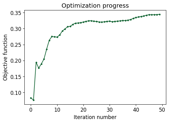
Plot the objective and the weighted contributions from each figure of merit and penalty.
fig, ax = plt.subplots(1, 1, figsize=(8, 4))

purcell_w = (
    purcell_target - anp.array(history_dict_2["purcell"])[:, center_idx]
) ** 2 * weight_purcell
coupling_w = anp.array(history_dict_2["coupling"])[:, center_idx] * weight_coupling
brightness_w = (
    anp.array(history_dict_2["brightness"])[:, center_idx] * weight_brightness
)
cross_w = -anp.array(history_dict_2["crosstalk"])[:, center_idx] * weight_cross
curve_pen_w = -anp.array(history_dict_2["curve_pen"]) * weight_curve_pen
minsep_pen_w = -anp.array(history_dict_2["min_sep_pen"]) * weight_minsep_pen
smooth_pen_w = -anp.array(history_dict_2["smoothness_pen"]) * weight_smooth
spacing_pen_w = -anp.array(history_dict_2["spacing_pen"]) * weight_spacing
border_pen_w = -anp.array(history_dict_2["border_dist_pen"]) * weight_border_dist

ax.plot(history_dict_2["values"], ".-", label="Objective")
ax.plot(purcell_w, ".-", label="Purcell (not included)")
ax.plot(coupling_w, ".-", label="Coupling")
ax.plot(brightness_w, ".-", label="Brightness (not included)")
ax.plot(cross_w, ".-", label="Crosstalk")
ax.plot(curve_pen_w, ".-", label="Curvature penalty")
ax.plot(minsep_pen_w, ".-", label="Min. sep. penalty")
ax.plot(smooth_pen_w, ".-", label="Smoothness penalty")
ax.plot(spacing_pen_w, ".-", label="Spacing penalty")
ax.plot(border_pen_w, ".-", label="Border dist. penalty")
ax.set_xlabel("Iteration number")
ax.set_ylabel("Contributions to objective")
ax.set_title("Objective function and contributions")

# Position legend to the right of the plot
ax.legend(loc="upper left", bbox_to_anchor=(1.05, 1))
# Adjust layout to prevent cutting off the legend
plt.tight_layout()
plt.show()
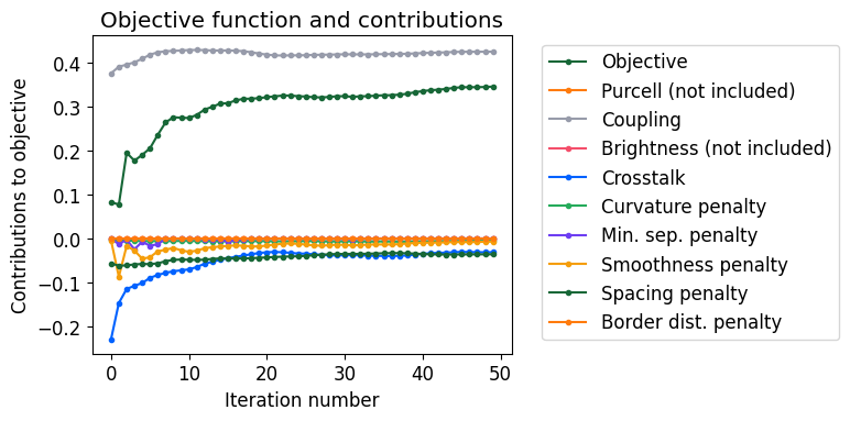
Figures of Merit Evolution
We can see how the figures of merit at the design wavelength have improved over the course of the optimization.
fig, (ax1, ax2, ax3) = plt.subplots(1, 3, figsize=(10, 4), tight_layout=True)

ax1.plot(
    anp.array(history_dict_2["purcell"])[:, center_idx], ".-", label="Purcell factor"
)
ax1.plot(anp.array(history_dict_2["coupling"])[:, center_idx], ".-", label="Coupling")
ax1.plot(
    anp.array(history_dict_2["brightness"])[:, center_idx], ".-", label="Brightness"
)
ax1.legend()
ax1.set_xlabel("Iteration number")

ax2.plot(anp.array(history_dict_2["crosstalk"])[:, center_idx], ".-", label="Crosstalk")
ax2.set_xlabel("Iteration number")
ax2.legend()

ax3.plot(history_dict_2["curve_pen"], ".-", label="Curvature penalty")
ax3.plot(history_dict_2["min_sep_pen"], ".-", label="Min. sep. penalty")
ax3.plot(history_dict_2["smoothness_pen"], ".-", label="Smoothness pen")
ax3.plot(history_dict_2["spacing_pen"], ".-", label="Spacing pen")
ax3.plot(history_dict_2["border_dist_pen"], ".-", label="Border dist. pen")
ax3.legend()
ax3.set_xlabel("Iteration number")

plt.show()
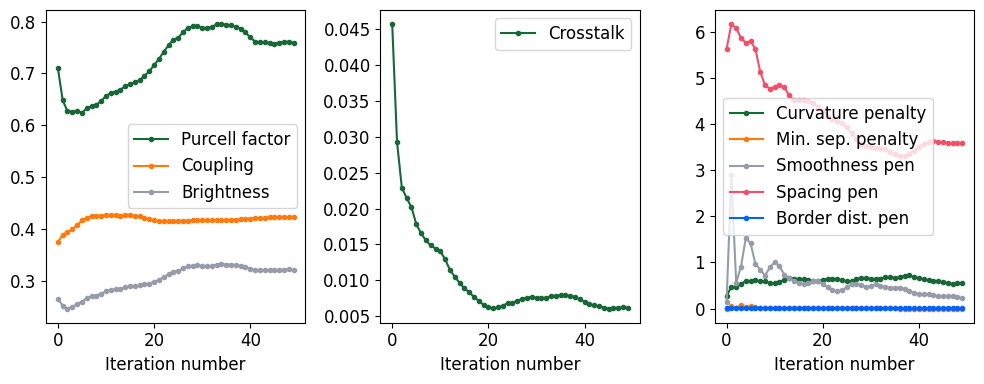
The coupling increases slightly and then asymptotes while the crosstalk decreases precipitously.
Final figures of merit at the design wavelength.
print(f"Final figures of merit at {wl * 1e3} nm:")
print(f"\tPurcell factor:\t{history_dict_2['purcell'][-1][center_idx]:.3f}")
print(f"\tCoupling:\t{100 * history_dict_2['coupling'][-1][center_idx]:.2f} %")
print(f"\tBrightness:\t{history_dict_2['brightness'][-1][center_idx]:.3f}")
print(f"\tCrosstalk:\t{100 * history_dict_2['crosstalk'][-1][center_idx]:.5f} %")
Final figures of merit at 798.0 nm:
	Purcell factor:	0.759
	Coupling:	42.38 %
	Brightness:	0.322
	Crosstalk:	0.62169 %
This is a significant improvement over the design from Stage 1 (coupling = 38%, crosstalk = 4.5%). The crosstalk, especially, has been improved.
Figures of Merit Spectra
Again we plot the spectral variations of the figures of merit to assess the performance of the final design.
fig, (ax1, ax2, ax3) = plt.subplots(1, 3, figsize=(10, 4), tight_layout=True)

ax1.plot(
    wl_range * 1000,
    anp.array(history_dict_2["purcell"])[-1, :],
    ".-",
    label="Purcell factor",
)
ax1.plot(
    wl_range * 1000,
    anp.array(history_dict_2["brightness"])[-1, :],
    ".-",
    label="Brightness",
)
ax1.legend()
ax1.set_xlabel("Wavelength (nm)")

ax2.plot(
    wl_range * 1000,
    anp.array(history_dict_2["coupling"])[-1, :],
    ".-",
    label="Coupling",
)
ax2.set_xlabel("Wavelength (nm)")
ax2.legend()

ax3.plot(
    wl_range * 1000,
    anp.array(history_dict_2["crosstalk"])[-1, :],
    ".-",
    label="Crosstalk",
)
ax3.set_xlabel("Wavelength (nm)")
ax3.legend()

plt.show()
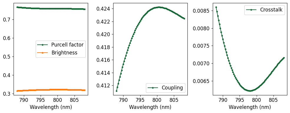
The extrema of the various figures of merit are located at or very near the design wavelength.
Figures of Merit Spectra Evolution
Plot the figures of merit as colormaps versus wavelength and iteration number.
purcell = anp.array(history_dict_2["purcell"])
coupling = anp.array(history_dict_2["coupling"])
crosstalk = anp.array(history_dict_2["crosstalk"])
wavelength, iteration = anp.meshgrid(
    wl_range * 1000, [j for j in range(len(purcell))], indexing="xy"
)

fig, axes = plt.subplots(1, 3, figsize=(12, 4))
quantities = [purcell, coupling, crosstalk]
titles = ["Purcell factor", "Coupling", "Crosstalk"]

for ax, quantity, title in zip(axes, quantities, titles):
    p = ax.pcolormesh(wavelength, iteration, quantity)  # , cmap="plasma")
    ax.set_xlabel("Wavelength (nm)")
    ax.set_ylabel("Iteration number")
    ax.set_title(title)
    plt.colorbar(p, ax=ax)

plt.tight_layout()
plt.show()
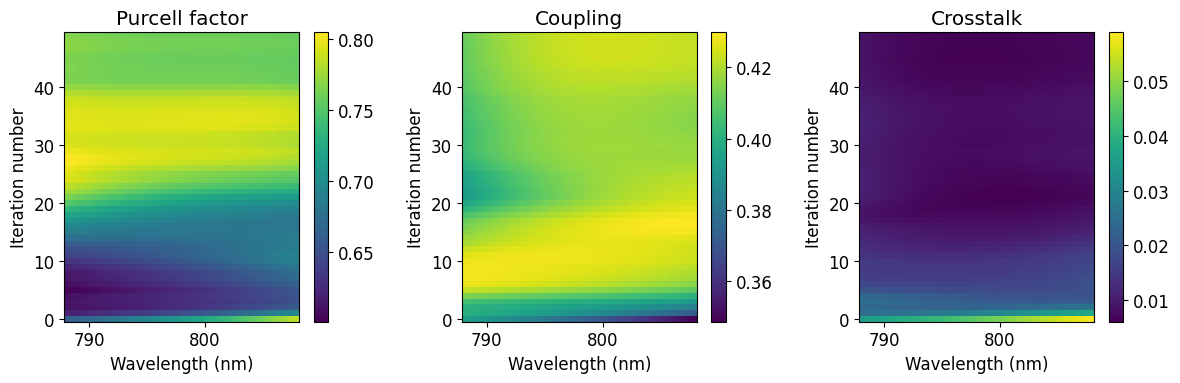
Close-up of Border
We can see that the final design is definitely different from the initial design. There are some wiggles in the outline that weren't there to begin with.
vertices_initial = make_reparam_vertices(reparams)
vertices_final = make_reparam_vertices(best_wgx_params)
control_points_final = make_control_points_from(best_wgx_params, smidge=0.020)
plt.plot(*anp.array(vertices_initial).T, "-")
plt.plot(*anp.array(vertices_final).T, "-")
plt.plot(*anp.array(control_points_final).T, ".")
ax = plt.gca()
ax.set_aspect("equal")
ax.set_xlabel("X (um)")
ax.set_ylabel("Y (um)")
ax.set_xlim((0, 0.8))
ax.set_ylim((0, 0.8))
plt.show()
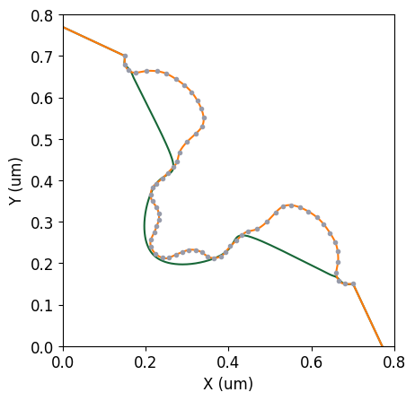
Animation of Optimization
It is interesting to watch how the WGX design changes during the optimization. It can also be helpful for troubleshooting if the optimization is not producing suitable designs.
from matplotlib.animation import FuncAnimation, PillowWriter
from IPython.display import HTML


def get_vertices(index):
    vertices = make_reparam_vertices(history_dict_2["params"][index])
    return vertices.T


# Set up the figure and axis
fig, ax = plt.subplots(figsize=(4, 4))
(line,) = ax.plot(*get_vertices(0))
ax.set_aspect("equal")


# Animation update function
def update(frame):
    line.set_data(*get_vertices(frame))
    return (line,)


# Build the FuncAnimation
frames = len(history_dict_2["params"])
interval = 50  # in ms
anim = FuncAnimation(fig, update, frames=frames, interval=interval, blit=True)

# Close the figure display here so it doesn’t show twice in notebook
plt.close(fig)

# Export as animated GIF via Pillow. Required by matplotlib, or run `pip install pillow`.
gif_writer = PillowWriter(fps=5)
filename = f"{WGX_adoint_run_title}_{run_number:02d}.gif"
figs_dir = Path("figs")
figs_dir.mkdir(parents=True, exist_ok=True)
fig_file = figs_dir / filename
anim.save(fig_file, writer=gif_writer)
print(f"Saved animation as {filename}")

# Display inline as HTML5 video (JS-based)
HTML(anim.to_jshtml())  # Must be the last line of the cell for it to display properly.
Saved animation as wgx_border_adjoint_20.gif
Final Crossing Design
cross_polyslab = make_reparam_polyslab(best_wgx_params)
cross_struct_2 = make_reparam_structure(best_wgx_params)
ax = cross_polyslab.plot(z=0)
ax.set_title("Final WGX design")
plt.show()
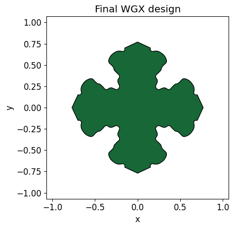
Field in the Final Design
sim_best = make_sim(best_wgx_params, use_fld_mnt=True)
sim_best_data = web.run(sim_best, task_name="final_wgx_adjoint_design", verbose=False)
f, ax = plt.subplots()
vminmax = 20000
huh = sim_best_data.plot_field(
    "field_xy", "Ey", ax=ax, vmin=-vminmax, vmax=vminmax, phase=0 * anp.pi
)
ax.set_title("Final adjoint design")
plt.show()
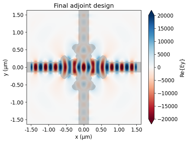
Animation of Field
from matplotlib.animation import FuncAnimation, PillowWriter
from IPython.display import HTML

# Set up the figure and axis
fig, ax = plt.subplots(figsize=(4, 4))

# Plot once to get everything in place
im = sim_best_data.plot_field(
    "field_xy", "Ey", ax=ax, vmin=-vminmax, vmax=vminmax, phase=0 * anp.pi
)
ax.set_title("Final adjoint design")
field_artist = im.get_children()[0]  # First child is the field QuadMesh object.

# Get the complex field array.
# Important to use .apply_phase because it interpolates the monitor data in the same way as .plot_field, above.
field_data = sim_best_data["field_xy"]
field_phi = field_data.apply_phase(anp.pi / 4)
Ey_complex = field_phi.Ey.values[:, :, 0, 0].T


# Change the phase of the (real) field
def field_at_phase(phi):
    """Return real part of field at phase phi."""
    return anp.real(Ey_complex * anp.exp(-1j * phi))


# Animation update function
vminmax = 10000
frames = 24
phase_array = anp.arange(frames) * 2 * anp.pi / frames


def update(frame):
    new_data = field_at_phase(phase_array[frame])
    field_artist.set_array(new_data.ravel())
    return (field_artist,)


# Build the FuncAnimation
interval = 50  # in ms
anim = FuncAnimation(fig, update, frames=frames, interval=interval, blit=True)

# Close the figure display here so it doesn’t show twice in notebook
plt.close(fig)

# Export as animated GIF via Pillow.  Required by matplotlib, or do `pip install pillow`.
gif_writer = PillowWriter(fps=5)
filename = f"{WGX_adoint_run_title}_{run_number:02d}_field_anim.gif"
figs_dir = Path("figs")
figs_dir.mkdir(parents=True, exist_ok=True)
fig_file = figs_dir / filename
anim.save(fig_file, writer=gif_writer)
print(f"Saved animation as {filename}")

# Display inline as HTML5 video (JS-based)
HTML(anim.to_jshtml())  # Must be the last line of the cell for it to display properly.
Saved animation as wgx_border_adjoint_20_field_anim.gif
Directional Power Analysis
To determine where the emitted power goes when it doesn't go into the output waveguides we can use the box of monitors around the dipole.
# Taking the code from the figures of merit function, we can calculate the total power radiated by the dipole.
dipole_power = anp.sum(
    anp.array(
        [anp.abs(sim_best_data[monitor.name].flux.values) for monitor in box_monitors]
    ),
    axis=0,
)
# Its shape is (81,), which is one value for every frequency recorded in the simulation.

box_fluxes = anp.array(
    [anp.abs(sim_best_data[monitor.name].flux.values) for monitor in box_monitors]
)
side_names = ["Left", "Right", "Bottom", "Top", "Down", "Up"]
power_fractions = 100 * box_fluxes[:, center_idx] / dipole_power[center_idx]
best_coupling_pct = 100 * history_dict_2["coupling"][-1][center_idx]
best_crosstalk_pct = 100 * history_dict_2["crosstalk"][-1][center_idx]

print(f"Side\tPower fraction at {wl * 1000:.0f} nm (%)")
print("-------------------------")
for side, fraction in zip(side_names, power_fractions):
    if side == "Left" or side == "Right":
        print(
            f"{side}:\t{fraction:.2f}\t\tCoupling: {best_coupling_pct:.2f}\t\tDifference: {fraction - best_coupling_pct:.2f}"
        )
    elif side == "Bottom" or side == "Top":
        print(
            f"{side}:\t{fraction:.2f}\t\tCrosstalk: {best_crosstalk_pct:.2f}\t\tDifference: {fraction - best_crosstalk_pct:.2f}"
        )
    else:
        print(f"{side}:\t{fraction:.2f}")
Side	Power fraction at 798 nm (%)
-------------------------
Left:	44.66		Coupling: 42.38		Difference: 2.28
Right:	44.66		Coupling: 42.38		Difference: 2.28
Bottom:	1.82		Crosstalk: 0.62		Difference: 1.20
Top:	1.82		Crosstalk: 0.62		Difference: 1.20
Down:	3.52
Up:	3.52
Stage 3: BO of PhC Mirrors
We have optimized the border of the WGX to maximize the coupling and minimize the crosstalk of a centrally located linear dipole. We can turn that device into a polarization demultiplexer ("poldemux") by adding photonic crystal (PhC) mirrors to two of the waveguides, reflecting the emission back into the two output waveguides. That requires optimizing the design of the PhC mirrors. For this step, we will use Bayesian optimization (BO) with a small parameter space, as it enables exploration of a relatively larger design space than adjoint optimization does. Later, in Stage 4, we can refine the best BO design with adjoint optimization.
This section of the notebook will cost ~4 flexcredits and take about an hour to run.Mirror Parameterization
Parameters for the PhC mirror:
- Dipole-to-mirror distance
- Mirror period
- Aspect ratio of elliptical holes
- Smallest ellipse y-diameter (for the hole closest to the dipole)
- Apodization distance
The hole closest to the dipole will start as the smallest, then each one will get bigger as determined by the apodization distance up to the maximum hole size, after which the holes will all be the same maximum size.
num_holes = (
    8  # We found that more than 8 holes did not change the eventual device performance.
)
min_hole_ydia = 0.100  # ensure the holes are not too small to fabricate
max_hole_ydia = 0.180  # ensure the holes won't cut the 0.3-um wide waveguide


def make_ellipse(center=(0.0, 0.0), dx=1.0, dy=1.0):
    """Use td.Polyslab on vertices produced via autograd.numpy functions."""
    num_angles = 36  # One vertex every 10 degrees
    angles = anp.arange(0, 2 * anp.pi, 1 / num_angles)
    vertices = []
    for angle in angles:
        x = dx / 2 * anp.cos(angle) + center[0]
        y = dy / 2 * anp.sin(angle) + center[1]
        vertices.append([x, y])
    return td.PolySlab(
        vertices=vertices, slab_bounds=(-wg_height / 2, wg_height / 2), axis=2
    )


def calc_hole_sizes(
    num_holes=8,
    mirror_period=0.170,
    aspect_ratio=1.0,
    smallest_hole_ydia=0.100,
    apo_dist=0.500,
):
    y_dias = []
    for j in range(num_holes):
        hole_ydia = (
            smallest_hole_ydia
            + j * (max_hole_ydia - smallest_hole_ydia) * mirror_period / apo_dist
        )
        y_dias.append(anp.min([hole_ydia, max_hole_ydia]))
    y_dias = anp.array(y_dias)
    x_dias = y_dias / aspect_ratio
    hole_sizes = [[x_dia, y_dia] for x_dia, y_dia in zip(x_dias, y_dias)]
    return hole_sizes


def make_mirror_geo(
    num_holes, mirror_dist, mirror_period, aspect_ratio, smallest_hole_ydia, apo_dist
):
    num_holes = int(num_holes)
    hole_sizes = calc_hole_sizes(
        num_holes, mirror_period, aspect_ratio, smallest_hole_ydia, apo_dist
    )
    x_list = -(mirror_dist + mirror_period * anp.arange(num_holes))
    hole_list = []
    for x, (x_dia, y_dia) in zip(x_list, hole_sizes):
        hole_list.append(make_ellipse((x, 0, 0), x_dia, y_dia))
    return td.GeometryGroup(geometries=hole_list)


def make_mirror_struct(
    num_holes, mirror_dist, mirror_period, aspect_ratio, smallest_hole_ydia, apo_dist
):
    mirror_geo = make_mirror_geo(
        num_holes,
        mirror_dist,
        mirror_period,
        aspect_ratio,
        smallest_hole_ydia,
        apo_dist,
    )
    return td.Structure(
        geometry=mirror_geo, background_medium=AlGaAs_simple, medium=vacuum
    )


def make_2_mirrors_struct(
    num_holes, mirror_dist, mirror_period, aspect_ratio, smallest_hole_ydia, apo_dist
):
    mirror_geo_1 = make_mirror_geo(
        num_holes,
        mirror_dist,
        mirror_period,
        aspect_ratio,
        smallest_hole_ydia,
        apo_dist,
    )
    mirror_geo_2 = mirror_geo_1.rotated(angle=anp.pi / 2, axis=2)
    mirror_group = td.GeometryGroup(geometries=[mirror_geo_1, mirror_geo_2])
    return td.Structure(
        geometry=mirror_group, background_medium=AlGaAs_simple, medium=vacuum
    )


# Example parameters
mirror_dist_guess = 0.800
mirror_period_guess = 0.180
aspect_ratio_guess = 2.0
smallest_hole_ydia_guess = 0.100
apo_dist_guess = 0.50
mirror_params_guess = [
    num_holes,
    mirror_dist_guess,
    mirror_period_guess,
    aspect_ratio_guess,
    smallest_hole_ydia_guess,
    apo_dist_guess,
]

two_mirrors_test = make_2_mirrors_struct(*mirror_params_guess)
ax = two_mirrors_test.plot(z=0)
ax.set_title("Example PhC mirror design")
plt.show()
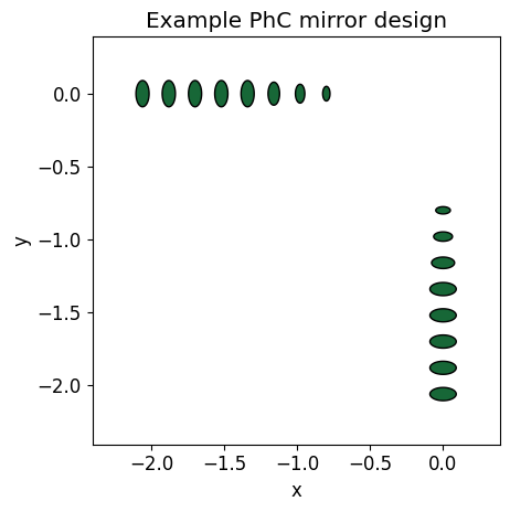
Plot the polyslabs all together so we can check that they overlap.
cross_polyslab = make_reparam_polyslab(best_wgx_params)
cross_struct_2 = make_reparam_structure(best_wgx_params)

ax = right_wg_box.plot(z=0)
top_wg_box.plot(z=0, ax=ax)
left_wg_box.plot(z=0, ax=ax)
bot_wg_box.plot(z=0, ax=ax)
cross_polyslab.plot(z=0, ax=ax)
two_mirrors_test.plot(z=0, ax=ax)

ax.set_xlim([-3, 3])
ax.set_ylim([-3, 3])
ax.set_title("Example poldemux design")
plt.show()
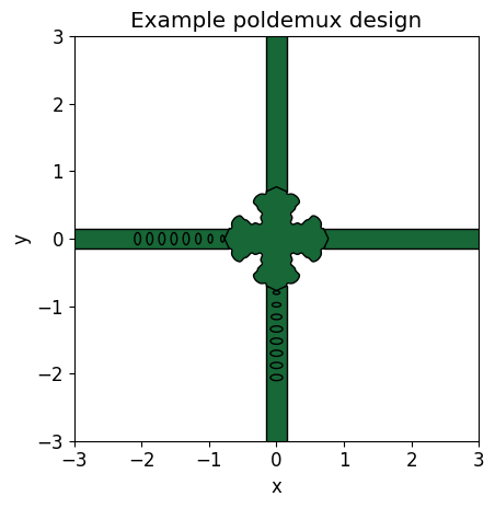
make_sim Function
def make_sim(
    mirror_params,
    use_fld_mnt: bool = True,
) -> td.Simulation:
    # Unravel the mirror parameters
    (
        num_holes,
        mirror_dist,
        mirror_period,
        aspect_ratio,
        smallest_hole_ydia,
        apo_dist,
    ) = mirror_params

    # Structures
    two_mirrors_struct = make_2_mirrors_struct(
        num_holes,
        mirror_dist,
        mirror_period,
        aspect_ratio,
        smallest_hole_ydia,
        apo_dist,
    )
    structures = static_structures + [cross_struct_2] + [two_mirrors_struct]

    # Sources and monitors
    sources = [dipole_src]
    monitors = [right_monitor, top_monitor] + box_monitors

    if use_fld_mnt == True:
        monitors = monitors + [field_monitor_xy]

    # Simulation size is the bounding box of the geometry modified by some multiple of pml_spacing.
    pml_spacing = 0.5
    sim_size = (
        1.0 * wg_length + cross_width - 1 * pml_spacing,
        1.0 * wg_length + cross_width - 1 * pml_spacing,
        wg_height + 2 * pml_spacing,
    )
    sim_origin = (
        -0.2 * wg_length,
        -0.2 * wg_length,
        0,
    )  # displaced to the left and down somewhat

    # Initialize simulation
    sim = td.Simulation(
        structures=structures,
        sources=sources,
        monitors=monitors,
        size=sim_size,
        center=sim_origin,
        grid_spec=grid_spec,
        run_time=run_time,
        boundary_spec=boundary_spec,
        symmetry=symmetry_B,
    )
    return sim


sim = make_sim(mirror_params=mirror_params_guess, use_fld_mnt=False)

fig, (ax1, ax2) = plt.subplots(1, 2, figsize=(10, 4), tight_layout=True)
sim.plot(z=0, ax=ax1)
sim.plot(x=0, ax=ax2)
plt.show()
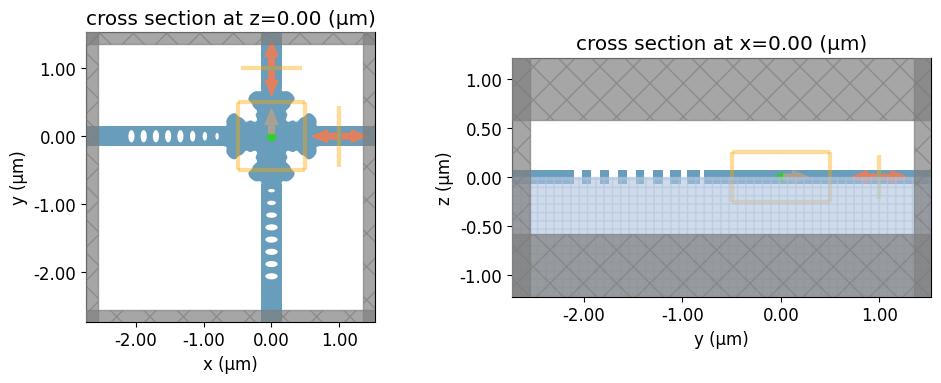
Optimization
Setup
DesignSpace
Tidy3D uses a DesignSpace object for gradient-free optimization approaches like Bayesian optimization, particle-swarm, and grid search.
# Bayesian optimization hyperparameters
initial_iter = 50  # To "prime" the Bayesian model
num_iter = 50  # number of iterations to refine the model
acq_func = "ucb"  # upper confidence bound, function used to choose next parameter set
kappa = 5.0  # higher means more exploration, lower means more exploitation. 5.0 is biased toward exploration.

# Design parameter spans
mirror_dist_span = (cross_width / 2, cross_width / 2 + 0.25)
mirror_period_span = (0.150, 0.200)
aspect_ratio_span = (0.9, 2.0)
smallest_hole_ydia_span = (min_hole_ydia, max_hole_ydia)
apo_dist_span = (
    0.1,
    1.0,
)  # minimum must not be zero to avoid a possible divide-by-zero error

mirror_dist = tdd.ParameterFloat(name="mirror_dist", span=mirror_dist_span)
mirror_period = tdd.ParameterFloat(name="mirror_period", span=mirror_period_span)
aspect_ratio = tdd.ParameterFloat(name="aspect_ratio", span=aspect_ratio_span)
smallest_hole_ydia = tdd.ParameterFloat(
    name="smallest_hole_ydia", span=smallest_hole_ydia_span
)
apo_dist = tdd.ParameterFloat(name="apo_dist", span=apo_dist_span)

# Assemble into a list to pass to tdd.DesignSpace
params = [mirror_dist, mirror_period, aspect_ratio, smallest_hole_ydia, apo_dist]

bayes_opt = tdd.MethodBayOpt(
    initial_iter=initial_iter, n_iter=num_iter, acq_func=acq_func, kappa=kappa
)

design_space = tdd.DesignSpace(
    method=bayes_opt, parameters=params, task_name="WGX_mirror_BO", path_dir="./data"
)

summary = design_space.summarize()
22:33:46 Eastern Daylight Time
                               Summary of DesignSpace

                               Method: MethodBayOpt
                               Method Args
                               initial_iter: 50
                               n_iter: 50
                               acq_func: ucb
                               kappa: 5.0
                               xi: 0.0

                               No. of Parameters: 5
                               Parameters: mirror_dist, mirror_period,
                               aspect_ratio, smallest_hole_ydia, apo_dist
                               mirror_dist: ParameterFloat (0.7, 0.95)
                               mirror_period: ParameterFloat (0.15, 0.2)
                               aspect_ratio: ParameterFloat (0.9, 2.0)
                               smallest_hole_ydia: ParameterFloat (0.1, 0.18)
                               apo_dist: ParameterFloat (0.1, 1.0)

                               Maximum Run Count: 100
History
# Directory and file in which to store optimization history
mirror_BO_run_title = "wgx_mirror_bayesopt"
history_name = f"{mirror_BO_run_title}_{run_number:02d}.pkl"
history_dir = Path("misc")
history_dir.mkdir(parents=True, exist_ok=True)
history_file_3 = history_dir / history_name

# Define a dictionary to store the history of the optimization
history_dict_3 = dict(
    values=[],
    purcell=[],
    coupling=[],
    brightness=[],
    crosstalk=[],
    mirror_params=[],
)
Pre-function
The pre-function will receive arguments suggested by the optimizer and return a Simulation object.
def dict_to_list(params):
    # MethodBayesOpt alphabetizes the parameters,
    # so we reorder them to match make_sim's expectation.
    param_list = [
        num_holes,
        params["mirror_dist"],
        params["mirror_period"],
        params["aspect_ratio"],
        params["smallest_hole_ydia"],
        params["apo_dist"],
    ]
    return param_list


def pre_func(**params):
    """Build a Simulation object from parameters suggested by the BO."""
    param_list = dict_to_list(params)
    # param_array = [num_holes] + list(params.values())
    sim = make_sim(mirror_params=param_list, use_fld_mnt=False)
    sim.attrs["mirror_params"] = param_list
    return sim
Post-function
During this stage of the overall optimization, we want to maximize the "brightness" of the light coupled into the output waveguide, which is the product of the coupling efficiency and the Purcell factor (which is in turn related to the power emitted by the dipole). The distance from the dipole to the mirror will affect the Purcell factor, which is why it is one of the design parameters to optimize.
# Brief description of the objective formula
obj_descr = "weighted brightness minus weighted crosstalk"

# Weights for dipole source
purcell_target = 100
weight_purcell = 0
weight_coupling = 0
weight_brightness = (
    1  # Brightness is the product of Purcell factor and coupling efficiency.
)
weight_cross = 5  # Strongly disincentivize crosstalk.


def post_func(sim_data: td.SimulationData) -> float:
    """Analyze SimulationData and return the objective value and auxiliary data."""
    purcell, coupling, brightness, crosstalk = dipole_figs_of_merit(sim_data)
    obj = (
        -((purcell_target - purcell[center_idx]) ** 2) * weight_purcell
        + coupling[center_idx] * weight_coupling
        + brightness[center_idx] * weight_brightness
        - crosstalk[center_idx] * weight_cross
    )

    # save history
    history_dict_3["values"].append(obj)
    history_dict_3["purcell"].append(purcell)
    history_dict_3["coupling"].append(coupling)
    history_dict_3["brightness"].append(brightness)
    history_dict_3["crosstalk"].append(crosstalk)
    history_dict_3["mirror_params"].append(
        sim_data.simulation.attrs["mirror_params"].copy()
    )  # Need to .copy otherwise all parameter sets are the same.
    save_history(history_dict_3, history_file_3)

    return [
        obj,
        {
            "purcell": purcell,
            "coupling": coupling,
            "brightness": brightness,
            "crosstalk": crosstalk,
        },
    ]
Metadata
# Metadata associated with the optimization and simulation setup
mirror_BO_metadata = dict(
    # Source
    center_wavelength=wl,
    bandwidth=bw,
    # Material
    index=n_AlGaAs,
    wg_height=wg_height,
    wg_width=wg_width,
    # Waveguide crossing
    cross_width=cross_width,
    smidge=smidge,
    num_vertices=num_vertices,
    control_points=best_wgx_params,
    # Mirror
    num_holes=num_holes,
    min_hole_ydia=min_hole_ydia,
    max_hole_ydia=max_hole_ydia,
    mirror_dist_span=mirror_dist_span,
    mirror_period_span=mirror_period_span,
    aspect_ratio_span=aspect_ratio_span,
    smallest_hole_ydia_span=smallest_hole_ydia_span,
    apo_dist_span=apo_dist_span,
    # Objective
    obj_descr=obj_descr,
    purcell_target=purcell_target,
    weight_purcell=weight_purcell,
    weight_coupling=weight_coupling,
    weight_brightness=weight_brightness,
    weight_cross=weight_cross,
    # BayesOpt hyperparameters
    initial_iter=initial_iter,
    num_iter=num_iter,
    acq_func=acq_func,
    kappa=kappa,
    pickle_file=history_name,
)

history_dict_3["mirror_BO_metadata"] = mirror_BO_metadata
Estimated Cost
cost_estimate = design_space.estimate_cost(
    pre_func
)  # Just uploads one job to get a cost estimate but doesn't run the job.
print(
    f"Estimated cost of BayesOpt using {initial_iter + num_iter} total simulations is {cost_estimate} flexcredits."
)
# Now we have to re-initialize the parameter and penalty history because pre_func added junk on this call.
history_dict_3["params"] = []
history_dict_3["border_dist_pen"] = []
22:34:04 Eastern Daylight Time Created task 'estimate_cost' with resource_id
                               'fdve-c831c55e-3c3a-40dd-96f0-ba9c200075bb' and
                               task_type 'FDTD'.
                               View task using web UI at
                               'https://tidy3d.simulation.cloud/workbench?taskId
                               =fdve-c831c55e-3c3a-40dd-96f0-ba9c200075bb'.
Task folder: 'default'.
Output()
22:34:09 Eastern Daylight Time Estimated FlexCredit cost: 0.042. Minimum cost
                               depends on task execution details. Use
                               'web.real_cost(task_id)' to get the billed
                               FlexCredit cost after a simulation run.
22:34:10 Eastern Daylight Time Estimated FlexCredit cost: 0.042. Minimum cost
                               depends on task execution details. Use
                               'web.real_cost(task_id)' to get the billed
                               FlexCredit cost after a simulation run.
Estimated cost of BayesOpt using 100 total simulations is 4.163 flexcredits.
Run the Optimization
# Took 54 minutes.
# 50 initial iterations took ~10 minutes. 50 more iterations took another 45 minutes.

td.config.logging_level = (
    "ERROR"  # Only give errors and ignore warnings to reduce clutter.
)

results = design_space.run(pre_func, post_func, verbose=True)

df = results.to_dataframe()
history_dict_3["df"] = df  # Add the dataframe of the results to the history...
save_history(history_dict_3, history_file_3)  # ...and save it.
22:34:46 Eastern Daylight Time Running 50 Simulations
22:43:37 Eastern Daylight Time Best Fit from Initial Solutions: 1.183
22:43:38 Eastern Daylight Time Running 1 Simulations
22:44:35 Eastern Daylight Time Running 1 Simulations
22:45:19 Eastern Daylight Time Running 1 Simulations
22:46:09 Eastern Daylight Time Running 1 Simulations
22:46:58 Eastern Daylight Time Running 1 Simulations
22:47:47 Eastern Daylight Time Running 1 Simulations
22:49:33 Eastern Daylight Time Running 1 Simulations
22:50:26 Eastern Daylight Time Running 1 Simulations
22:51:14 Eastern Daylight Time Running 1 Simulations
22:51:59 Eastern Daylight Time Running 1 Simulations
22:52:44 Eastern Daylight Time Running 1 Simulations
22:53:33 Eastern Daylight Time Running 1 Simulations
22:54:20 Eastern Daylight Time Running 1 Simulations
22:55:08 Eastern Daylight Time Running 1 Simulations
22:55:55 Eastern Daylight Time Running 1 Simulations
22:56:59 Eastern Daylight Time Running 1 Simulations
22:57:48 Eastern Daylight Time Running 1 Simulations
22:58:49 Eastern Daylight Time Running 1 Simulations
22:59:38 Eastern Daylight Time Running 1 Simulations
23:00:23 Eastern Daylight Time Running 1 Simulations
23:01:14 Eastern Daylight Time Running 1 Simulations
23:02:03 Eastern Daylight Time Running 1 Simulations
23:02:53 Eastern Daylight Time Running 1 Simulations
23:03:42 Eastern Daylight Time Running 1 Simulations
23:04:29 Eastern Daylight Time Running 1 Simulations
23:05:18 Eastern Daylight Time Running 1 Simulations
23:06:30 Eastern Daylight Time Running 1 Simulations
23:07:17 Eastern Daylight Time Running 1 Simulations
23:09:29 Eastern Daylight Time Running 1 Simulations
23:10:50 Eastern Daylight Time Running 1 Simulations
23:11:37 Eastern Daylight Time Running 1 Simulations
23:12:23 Eastern Daylight Time Running 1 Simulations
23:13:10 Eastern Daylight Time Running 1 Simulations
23:13:56 Eastern Daylight Time Running 1 Simulations
23:14:47 Eastern Daylight Time Running 1 Simulations
23:15:44 Eastern Daylight Time Running 1 Simulations
23:16:53 Eastern Daylight Time Running 1 Simulations
23:17:40 Eastern Daylight Time Running 1 Simulations
23:18:31 Eastern Daylight Time Running 1 Simulations
23:19:19 Eastern Daylight Time Running 1 Simulations
23:20:08 Eastern Daylight Time Running 1 Simulations
23:20:59 Eastern Daylight Time Running 1 Simulations
23:21:48 Eastern Daylight Time Running 1 Simulations
23:23:07 Eastern Daylight Time Running 1 Simulations
23:23:56 Eastern Daylight Time Running 1 Simulations
23:24:40 Eastern Daylight Time Running 1 Simulations
23:25:31 Eastern Daylight Time Running 1 Simulations
23:26:16 Eastern Daylight Time Running 1 Simulations
23:27:09 Eastern Daylight Time Running 1 Simulations
23:27:54 Eastern Daylight Time Running 1 Simulations
23:28:47 Eastern Daylight Time Best Result: 1.1831005269631318
                               Best Parameters: apo_dist: 0.6692750256302317
                               aspect_ratio: 1.999507791764609 mirror_dist:
                               0.726680862143243 mirror_period:
                               0.1589803868641277 smallest_hole_ydia:
                               0.16766765667327527
Confirm Cost
# For a BO, num_tasks is:
num_tasks = initial_iter + num_iter

# Get the task information for the last num_tasks simulations.
task_dict_list = web.api.webapi.get_tasks(num_tasks)
cost_array = []
for task_dict in task_dict_list:
    cost_array.append(
        task_dict["realFlexUnit"]
    )  # The real cost is contained in the task dictionary
cost_array = anp.array(cost_array)
total_cost = anp.cumsum(cost_array)[-1]  # Sum the costs of all the simulations

# Might as well save the task information, too.
history_dict_3["task_dict_list"] = task_dict_list
save_history(history_dict_3, history_file_3)

print(f"Total cost of the optimization run: {total_cost:.4f} flexcredits")
Total cost of the optimization run: 3.7178 flexcredits
Analyzing Mirror BO Results
Metadata
mirror_BO_metadata
{'center_wavelength': 0.798,
 'bandwidth': 0.02,
 'index': np.float64(3.5693094750241627),
 'wg_height': 0.15,
 'wg_width': 0.3,
 'cross_width': 1.4,
 'smidge': 0.02,
 'num_vertices': 600,
 'control_points': array([0.66570807, 0.15824534, 0.65945441, 0.17607427, 0.66358888,
        0.2017893 , 0.66296506, 0.22785962, 0.65738362, 0.24968094,
        0.64457273, 0.27254689, 0.62949765, 0.29349163, 0.6123603 ,
        0.31107846, 0.59225935, 0.32480425, 0.57203275, 0.33448017,
        0.55066454, 0.33992201, 0.53071576, 0.33648086, 0.51344627,
        0.32217333, 0.4928945 , 0.30017632, 0.46779913, 0.28193745,
        0.44619447, 0.27651754, 0.43147051, 0.26685128, 0.41815579,
        0.2539781 , 0.4044092 , 0.24074104, 0.39213216, 0.22611728,
        0.38156116, 0.2162635 , 0.36504075, 0.21223107, 0.34958276,
        0.21615437, 0.33588618, 0.22582844, 0.32069805, 0.23157984,
        0.3038986 , 0.23186402, 0.28919542, 0.22685626, 0.27403823,
        0.2208185 , 0.25638795, 0.21284513, 0.24067806, 0.21288161,
        0.22314173]),
 'num_holes': 8,
 'min_hole_ydia': 0.1,
 'max_hole_ydia': 0.18,
 'mirror_dist_span': (0.7, 0.95),
 'mirror_period_span': (0.15, 0.2),
 'aspect_ratio_span': (0.9, 2.0),
 'smallest_hole_ydia_span': (0.1, 0.18),
 'apo_dist_span': (0.1, 1.0),
 'obj_descr': 'weighted brightness minus weighted crosstalk',
 'purcell_target': 100,
 'weight_purcell': 0,
 'weight_coupling': 0,
 'weight_brightness': 1,
 'weight_cross': 5,
 'initial_iter': 50,
 'num_iter': 50,
 'acq_func': 'ucb',
 'kappa': 5.0,
 'pickle_file': 'wgx_mirror_bayesopt_20.pkl'}
We can view the objective function ("output") for each set of design parameters.
df
| apo_dist | aspect_ratio | mirror_dist | mirror_period | smallest_hole_ydia | output | |
|---|---|---|---|---|---|---|
| 0 | 0.508763 | 1.748670 | 0.751145 | 0.170498 | 0.115471 | 0.449019 |
| 1 | 0.720361 | 1.149394 | 0.703644 | 0.191765 | 0.106979 | 1.137908 |
| 2 | 0.889080 | 1.048320 | 0.789801 | 0.180207 | 0.112757 | -0.106060 |
| 3 | 0.612707 | 1.476591 | 0.758129 | 0.180722 | 0.130630 | 0.394074 |
| 4 | 0.556047 | 1.713638 | 0.813138 | 0.150735 | 0.126886 | -0.058971 |
| ... | ... | ... | ... | ... | ... | ... |
| 95 | 0.647420 | 2.000000 | 0.760320 | 0.200000 | 0.142832 | -0.114104 |
| 96 | 0.777964 | 1.979105 | 0.813565 | 0.190961 | 0.137716 | 0.652760 |
| 97 | 0.240180 | 1.959360 | 0.700000 | 0.150304 | 0.143999 | 0.690048 |
| 98 | 0.226256 | 1.967840 | 0.700000 | 0.200000 | 0.180000 | 1.062789 |
| 99 | 0.742982 | 1.976006 | 0.700000 | 0.150000 | 0.140194 | 0.582734 |
100 rows × 6 columns
Best Design
Sort the output and plot the top 5 best-performing designs.
top_N = 5
df_sorted = df.sort_values(by=["output"])
# Reorder because MethodBayesOpt alphabetizes the parameters.
df_sorted = df_sorted.reindex(
    columns=[
        "mirror_dist",
        "mirror_period",
        "aspect_ratio",
        "smallest_hole_ydia",
        "apo_dist",
        "output",
    ]
)
param_array = df_sorted.to_numpy()[-top_N:, :-1]
param_array = param_array[::-1]  # best to worst
best_mirror_params = anp.array([num_holes] + [el for el in param_array[0]])

# Plot from best to top_Nth best
fig, axs = plt.subplots(1, top_N, figsize=(10, 4), tight_layout=True)
for ax, top_params in zip(axs, param_array):
    mirror_params = [num_holes] + [el for el in top_params]
    mirror_struct = make_mirror_struct(*mirror_params)
    ax = mirror_struct.plot(z=0, ax=ax)
    ax.set_title("")
    ax.set_xlabel("")
    ax.set_ylabel("")

print(f"Objective values: {df_sorted.to_numpy()[-top_N:, -1][::-1]}")
plt.show()
Objective values: [1.18310053 1.17715128 1.15905647 1.15865493 1.15776294]

For reference, here are the design parameters for the five best designs.
param_array
array([[0.72668086, 0.15898039, 1.99950779, 0.16766766, 0.66927503],
       [0.71768138, 0.18247298, 1.92603661, 0.17079866, 0.23522049],
       [0.7       , 0.2       , 1.8961487 , 0.13464245, 0.29545233],
       [0.7       , 0.2       , 1.98679058, 0.1574577 , 0.65578267],
       [0.7       , 0.2       , 1.84761771, 0.13372078, 0.38153961]])
(
    best_num_holes,
    best_mirror_dist,
    best_mirror_period,
    best_aspect_ratio,
    best_smallest_hole_ydia,
    best_apo_dist,
) = best_mirror_params
print("Best parameters:")
print(f"\tnum_holes\t= {best_num_holes:.0f} (fixed)")
print(f"\tmirror_dist\t= {best_mirror_dist:.6f}")
print(f"\tmirror_period\t= {best_mirror_period:.6f}")
print(f"\taspect_ratio\t= {best_aspect_ratio:.6f}")
print(f"\tsmallest_hole_ydia = {best_smallest_hole_ydia:.6f}")
print(f"\tapo_dist\t= {best_apo_dist:.6f}")
Best parameters:
	num_holes	= 8 (fixed)
	mirror_dist	= 0.726681
	mirror_period	= 0.158980
	aspect_ratio	= 1.999508
	smallest_hole_ydia = 0.167668
	apo_dist	= 0.669275
Figures of Merit Spectra
best_idx = anp.argmax(anp.array(results.values))
best_aux_values_3 = results.aux_values[best_idx]

fig, (ax1, ax2, ax3) = plt.subplots(1, 3, figsize=(10, 4), tight_layout=True)

ax1.plot(
    wl_range * 1000,
    anp.array(best_aux_values_3["purcell"]),
    ".-",
    label="Purcell factor",
)
ax1.plot(
    wl_range * 1000,
    anp.array(best_aux_values_3["brightness"]),
    ".-",
    label="Brightness",
)
ax1.legend()
ax1.set_xlabel("Wavelength (nm)")

ax2.plot(
    wl_range * 1000, anp.array(best_aux_values_3["coupling"]), ".-", label="Coupling"
)
ax2.set_xlabel("Wavelength (nm)")
ax2.legend()

ax3.plot(
    wl_range * 1000, anp.array(best_aux_values_3["crosstalk"]), ".-", label="Crosstalk"
)
ax3.set_xlabel("Wavelength (nm)")
ax3.legend()

print(f"Figures of merit at {wl * 1000:.0f} nm")
print(f"\tPurcell factor = {best_aux_values_3['purcell'][center_idx]}")
print(f"\tCoupling eff.  = {best_aux_values_3['coupling'][center_idx]}")
print(f"\tBrightness     = {best_aux_values_3['brightness'][center_idx]}")
print(f"\tCrosstalk      = {best_aux_values_3['crosstalk'][center_idx]}")

plt.show()
Figures of merit at 798 nm
	Purcell factor = 1.3767564252294884
	Coupling eff.  = 0.8798245164801979
	Brightness     = 1.2113040561385404
	Crosstalk      = 0.005640705835081736
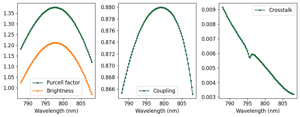
Now that there are mirrors in two of the waveguides, the coupling is approximately twice as high (now 88% compared to 42% after Stage 2). The Purcell effect is now greater than unity, indicating that the dipole emits more power than it would in an unpatterned bulk material. This is the effect of the mirror confining the light on one side. The crosstalk is still less than 1% across the whole bandwidth.
Fields in the Final Design
sim_best = make_sim(best_mirror_params, use_fld_mnt=True)
sim_best_data = web.run(sim_best, task_name="WGX_best_mirror", verbose=False)
f, ax = plt.subplots()
vminmax = 10000
sim_best_data.plot_field("field_xy", "Ey", ax=ax, vmin=-vminmax, vmax=vminmax)
ax.set_title("Final BO poldemux design")
plt.show()
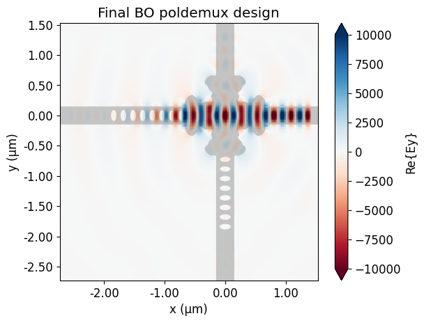
Animation of Field
from matplotlib.animation import FuncAnimation, PillowWriter
from IPython.display import HTML

# Set up the figure and axis
fig, ax = plt.subplots(figsize=(6, 4))

# Plot once to get everything in place
im = sim_best_data.plot_field(
    "field_xy", "Ey", ax=ax, vmin=-vminmax, vmax=vminmax, phase=0 * anp.pi
)
ax.set_title("Best BO mirror design")
field_artist = im.get_children()[0]  # First child is the field QuadMesh object.

# Get the complex field array.
# Important to use .apply_phase because it interpolates the monitor data in the same way as .plot_field, above.
field_data = sim_best_data["field_xy"]
field_phi = field_data.apply_phase(anp.pi / 4)
Ey_complex = field_phi.Ey.values[:, :, 0, 0].T


# Change the phase of the (real) field
def field_at_phase(phi):
    """Return real part of field at phase phi."""
    return anp.real(Ey_complex * anp.exp(-1j * phi))


# Animation update function
vminmax = 10000
frames = 24
phase_array = anp.arange(frames) * 2 * anp.pi / frames


def update(frame):
    new_data = field_at_phase(phase_array[frame])
    field_artist.set_array(new_data.ravel())
    return (field_artist,)


# Build the FuncAnimation
interval = 50  # in ms
anim = FuncAnimation(fig, update, frames=frames, interval=interval, blit=True)

# Close the figure display here so it doesn’t show twice in notebook
plt.close(fig)

# Export as animated GIF via Pillow.  Required by matplotlib, or do `pip install pillow`.
gif_writer = PillowWriter(fps=5)
filename = f"{mirror_BO_run_title}_{run_number:02d}_field_anim.gif"
figs_dir = Path("figs")
figs_dir.mkdir(parents=True, exist_ok=True)
fig_file = figs_dir / filename
anim.save(fig_file, writer=gif_writer)
print(f"Saved animation as {filename}")

# Display inline as HTML5 video (JS-based)
HTML(anim.to_jshtml())  # Must be the last line of the cell for it to display properly.
Saved animation as wgx_mirror_bayesopt_20_field_anim.gif
Directional Power Analysis
# Taking the code from the figures of merit function, we can calculate the total power radiated by the dipole.
dipole_power = anp.sum(
    anp.array(
        [anp.abs(sim_best_data[monitor.name].flux.values) for monitor in box_monitors]
    ),
    axis=0,
)
# Its shape is (81,), which is one value for every frequency recorded in the simulation.

box_fluxes = anp.array(
    [anp.abs(sim_best_data[monitor.name].flux.values) for monitor in box_monitors]
)
side_names = ["Left", "Right", "Bottom", "Top", "Down", "Up"]
power_fractions = 100 * box_fluxes[:, center_idx] / dipole_power[center_idx]
print("Side\tPower fraction (%)")
print("-------------------------")
for side, fraction in zip(side_names, power_fractions):
    if side == "Right":
        print(
            f"{side}:\t{fraction:.2f}\tCoupling: {100 * best_aux_values_3['coupling'][center_idx]:.2f}\t\tDifference: {fraction - 100 * best_aux_values_3['coupling'][center_idx]:.2f}"
        )
    elif side == "Bottom" or side == "Top":
        print(
            f"{side}:\t{fraction:.2f}\tCrosstalk: {100 * best_aux_values_3['crosstalk'][center_idx]:.2f}\t\tDifference: {fraction - 100 * best_aux_values_3['crosstalk'][center_idx]:.2f}"
        )
    else:
        print(f"{side}:\t{fraction:.2f}")
Side	Power fraction (%)
-------------------------
Left:	1.64
Right:	90.44	Coupling: 87.98		Difference: 2.45
Bottom:	1.59	Crosstalk: 0.56		Difference: 1.02
Top:	1.73	Crosstalk: 0.56		Difference: 1.17
Down:	2.30
Up:	2.30
The fractions of power exiting the six sides of the field monitor box around the dipole show where the lost emission is going. The vast majority (88%) of the emitted power is going out the output waveguide. About 2% more is going in that direction but not in the waveguide. A relatively small 1.6% is going to the left. About 4.6% of the total power goes out of the plane of the device. Only 3.3% of the total power goes in the directions of the top and bottom waveguides, though only 0.6% of the total power is confined in the top waveguide.
Stage 4: Simultaneous Adjoint Optimization of WGX Border and PhC Mirror
We will start with the adjoint-optimized WGX border from Stage 2 and the mirror design from Stage 3. That design will be the initial condition for simultaneous adjoint optimization of the WGX border and the PhC mirror holes. We will also allow the border to follow the reduced symmetry of the system with mirrors. That is, a single diagonal mirror plane rather than 4-fold rotational symmetry and four mirror planes (as in Stage 2 when the WGX had no mirrors).
This section of the notebook will cost about 4 flexcredits and take about 5 hours to run.WGX Symmetry Reduction
The diagonal mirror symmetry of the WGX with mirrors means that the four quadrants of the WGX need not all be the same. The upper-right and lower-left quadrants can be different, though each is individually even-symmetric across the diagonal y=x. The upper-left and lower-right quadrants will be mirror images of each other, but can be different from the other two quadrants.
This reduction in symmetry necessitates an increase in the number of control point parameters that characterize the WGX border. At first, all the quadrants will be identical because that is the design inherited from the WGX adjoint optimization in Stage 2.
We need structure parameters for:
- 1/2 border for quadrant 1, including one value for the diagonal point's x and y coordinates.
- full border for quadrant 2, where the diagonal point gets independent x and y coordinates (quadrant 4 is a mirrored copy of this)
- 1/2 border for quadrant 3, including one value for the diagonal point's x and y coordinates.
The simplest approach is to separate the best_wgx_params into an array of x positions, an array of y positions, and the diagonal coordinate. Then use list comprehensions to create the other required parameter arrays. Later, another function will create full borders for all quadrants from these parameters.
num_free_pts = 30
num_vertices = 600  # along one quarter of the device border

# Separate the parameters from the 1/8th of the WGX border represented by best_wgx_params.
x_coords = best_wgx_params[:-1:2]  # x coords of all but the diagonal point
y_coords = best_wgx_params[1:-1:2]  # y coords of all but the diagonal point
diag = best_wgx_params[-1]  # the diagonal point's x and y position

# Parameters for quadrant 1 (upper-right). Symmetry means only half of this quadrant is independent
params_quad1 = (
    best_wgx_params  # num_free_pts pairs of (x, y) coords plus one diagonal y=x coord
)

# Parameters for quadrant 2 and quadrant 4 (upper-left and lower-right)
coords_quad2 = [[-y, x] for x, y in zip(x_coords, y_coords)] + [[-diag, diag]]
coords_quad2 = coords_quad2 + [[-x, y] for x, y in zip(x_coords[::-1], y_coords[::-1])]
coords_quad2 = anp.array(coords_quad2)
params_quad2 = coords_quad2.flatten()  # 2*num_free_pts+1 pairs of (x, y) coords

# Parameters for quadrant 3 (lower-left)
params_quad3 = (
    -best_wgx_params
)  # num_free_pts pairs of (x, y) coords plus one diagonal y=x coord

# Assemble the array of parameters for all four quadrants of the border
initial_border_params = anp.array(
    list(params_quad1) + list(params_quad2) + list(params_quad3)
)
Below are functions to do the following:
- Extract the parameters corresponding to a given quadrant from the
border_params. - Return the control points for each quadrant of the border, including the waveguide corner and the "smidge" point.
- Return the vertices for each quadrant of the border.
- Take the vertices for each quadrant of the border, add the "pinning points", and concatenate them into one array to make a polyslab and/or structure.
def quadrant_ctrl_pts_from(border_params, quad, smidge=0.020):
    """
    border_params (NDarray): 8*num_control_pts+2 design parameters
    quad (int): quadrant index: 1, 2, 3, or 4
    smidge (float): X-distance between the fixed control point on the corner of the waveguide and the fixed neighboring point.
    """

    # Fixed points at and near the waveguide corner
    p_corner = anp.array([[cross_width / 2, wg_width / 2]])
    p_2 = p_corner - anp.array([[smidge, 0]])

    # Extract the parameters for just one quadrant
    if quad == 1:
        # Extract the parameters for the first quadrant (upper-right)
        quadrant_params = border_params[: 2 * num_free_pts + 1]
        # Coords of the point along the diagonal
        p_mid = anp.array([[quadrant_params[-1], quadrant_params[-1]]])
        # Coords of the free points between the corner and the diagonal
        p_others = quadrant_params[:-1].reshape([-1, 2])
        # Put the coords all together, including the fixed points near the waveguide corner
        control_points = anp.concatenate((p_corner, p_2, p_others, p_mid))
        mirrored_points = control_points[-2::-1, ::-1]
        control_points = anp.concatenate((control_points, mirrored_points))
    elif quad == 2 or quad == 4:
        # Extract the parameters for the second and fourth quadrants (upper-left and lower-right)
        quadrant_params = border_params[
            2 * num_free_pts + 1 : 3 * (2 * num_free_pts + 1)
        ]
        # Coords of the free points
        p_free = quadrant_params.reshape([-1, 2])
        # Put the coords all together with the fixed points near the waveguide corners
        control_points = anp.concatenate(
            (
                anp.array([[-wg_width / 2, cross_width / 2]]),
                anp.array([[-wg_width / 2, cross_width / 2 - smidge]]),
                p_free,
                anp.array([[-cross_width / 2 + smidge, wg_width / 2]]),
                anp.array([[-cross_width / 2, wg_width / 2]]),
            )
        )
        if quad == 4:
            control_points = -control_points
    elif quad == 3:
        # Extract the parameters for the third quadrant (lower-left)
        quadrant_params = border_params[3 * (2 * num_free_pts + 1) :]
        # Coords of the point along the diagonal
        p_mid = anp.array([[quadrant_params[-1], quadrant_params[-1]]])
        # Coords of the free points between the corner and the diagonal
        p_others = quadrant_params[:-1].reshape([-1, 2])
        # Put the coords all together, including the fixed points near the waveguide corner
        control_points = anp.concatenate((-p_corner, -p_2, p_others, p_mid))
        mirrored_points = control_points[-2::-1, ::-1]
        control_points = anp.concatenate((control_points, mirrored_points))

    return control_points


def quadrant_vertices_from(border_params, quad, smidge=0.020, num_vertices=600):
    """
    Returns the vertices for one quadrant of the WGX border.
    """
    control_points = quadrant_ctrl_pts_from(border_params, quad, smidge)
    N_ctrl = len(control_points)
    x_ctrl = control_points[:, 0]
    y_ctrl = control_points[:, 1]
    t_ctrl = anp.linspace(0.0, 1.0, N_ctrl)
    order = 3
    _, x_eval = interpolate_spline(t_ctrl, x_ctrl, order=order, num_points=num_vertices)
    _, y_eval = interpolate_spline(t_ctrl, y_ctrl, order=order, num_points=num_vertices)
    quadrant_vertices = anp.stack([x_eval, y_eval], axis=-1)
    return quadrant_vertices


def all_vertices_from(border_params, smidge=0.020, num_vertices=600):
    """
    Returns the vertices of the whole WGX.
    """
    # Single points at the tip of each arm of the WGX ensure it attaches to the waveguides.
    pin_factor = 1.05  # Controls depth into the waveguide of the "point" ensuring the cross attaches to the waveguide.
    right_point = anp.array([[cross_width / 2 * pin_factor, 0]])
    top_point = anp.array([[0, cross_width / 2 * pin_factor]])
    left_point = anp.array([[-cross_width / 2 * pin_factor, 0]])
    bot_point = anp.array([[0, -cross_width / 2 * pin_factor]])

    upper_right = quadrant_vertices_from(border_params, 1, smidge, num_vertices)
    upper_left = quadrant_vertices_from(border_params, 2, smidge, num_vertices)
    lower_left = quadrant_vertices_from(border_params, 3, smidge, num_vertices)
    lower_right = quadrant_vertices_from(border_params, 4, smidge, num_vertices)

    vertices = anp.concatenate(
        [
            right_point,
            upper_right,
            top_point,
            upper_left,
            left_point,
            lower_left,
            bot_point,
            lower_right,
        ]
    )

    return vertices


# Helper functions
def make_wgx_polyslab(border_params: anp.ndarray, smidge, num_vertices) -> td.PolySlab:
    """Make a `tidy3d.PolySlab` for the device given the design parameters."""
    wgx_vertices = all_vertices_from(border_params, smidge, num_vertices)
    return td.PolySlab(
        vertices=wgx_vertices, slab_bounds=(-wg_height / 2, wg_height / 2), axis=2
    )


def make_wgx_structure(
    border_params: anp.ndarray, smidge, num_vertices
) -> td.Structure:
    wgx_polyslab = make_wgx_polyslab(border_params, smidge, num_vertices)
    return td.Structure(geometry=wgx_polyslab, medium=AlGaAs_simple, name="wgx border")


wgx_polyslab = make_wgx_polyslab(initial_border_params, smidge, num_vertices)
ax = wgx_polyslab.plot(z=0)
ax.set_title("WGX design before simultaneous optim.")
plt.show()
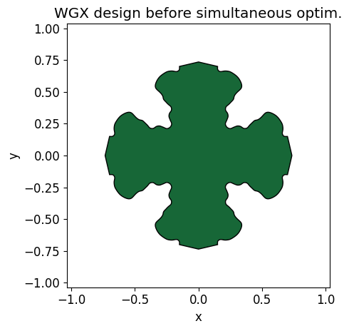
Mirror Re-parameterization for Adjoint Optimization
The adjoint optimization design parameters for the mirror will be independent for each hole. To avoid potential issues with hole overlap, holes too small, or "bridges" between holes too thin, we will parameterize the mirror holes using the hole widths and "bridge" widths between the holes. Then we use sigmoid limiting functions to bound the possible values of the hole and bridge widths while leaving the corresponding design parameters unbounded. This is simpler than incorporating a fabrication penalty to prevent the holes and bridges from being too small.
Thus, the structure parameters will be:
- Distance from the dipole to the edge of the first hole.
- Hole x-widths.
- "Bridge" widths between the holes (there will be
num_holes$-1$ of these). - Hole y-widths (This must be limited to 0.180 microns or less so as not to cut the waveguide apart.)
(Note that x-width and y-width here refer to the holes in the left waveguide. Those in the bottom waveguide are just mirror images.)
We must translate the simpler parameterization from Stage 3 into a version for adjoint optimization.
Inside the function make_mirror_geo, above, there are two lines that will give us the sizes and axial positions of the mirror holes. We will use those to obtain the initial structure parameters.
# Obtain info from the BO mirror parameters
(
    best_num_holes,
    best_mirror_dist,
    best_mirror_period,
    best_aspect_ratio,
    best_smallest_hole_ydia,
    best_apo_dist,
) = best_mirror_params
hole_sizes = anp.array(
    calc_hole_sizes(
        num_holes=int(best_num_holes),
        mirror_period=best_mirror_period,
        aspect_ratio=best_aspect_ratio,
        smallest_hole_ydia=best_smallest_hole_ydia,
        apo_dist=best_apo_dist,
    )
)
x_list = -(best_mirror_dist + best_mirror_period * anp.arange(best_num_holes))

# Find the new structure parameters
hole_x_widths = anp.array([x_width for x_width in hole_sizes[:, 0]])
hole_y_widths = anp.array([y_width for y_width in hole_sizes[:, 1]])
dipole_mirror_dist = anp.array([-x_list[0] - hole_x_widths[0] / 2])
bridge_widths = -anp.diff(x_list) - hole_x_widths[0:-1] / 2 - hole_x_widths[1:] / 2

initial_structure_params = (
    dipole_mirror_dist,
    hole_x_widths,
    hole_y_widths,
    bridge_widths,
)

# Choose allowable ranges of the structure parameters.
# Ensure that these span encompass the initial parameters, otherwise errors will occur later.
dipole_mirror_dist_span = (0.300, 1.5)
hole_x_width_span = (0.068, 0.500)
hole_y_width_span = (min_hole_ydia, max_hole_ydia + 0.005)
bridge_width_span = (0.068, 0.500)
We need to relate the structure parameters (which are bounded by the spans defined above) to unbounded design parameters using a sigmoid function. We only need to do that once to obtain the initial mirror design parameters for the adjoint optimization. We also want to be able to do the reverse: produce bounded structure parameters from unbounded design parameters. This second process is what will be done to create the tidy.Structure for the mirror from the design parameters.
def sigmoid(x, span):
    min, max = span
    norm_sig = 1 / (1 + anp.exp(-x))
    return min + (max - min) * norm_sig


def un_sigmoid(y, span):
    min, max = span
    return -anp.log((max - min) / (y - min) - 1)


def structure_params_from(mirror_design_params):
    qd_mirror_dist = sigmoid(mirror_design_params[0], dipole_mirror_dist_span)
    hole_x_widths = sigmoid(mirror_design_params[1 : num_holes + 1], hole_x_width_span)
    hole_y_widths = sigmoid(
        mirror_design_params[num_holes + 1 : 2 * num_holes + 1], hole_y_width_span
    )
    bridge_widths = sigmoid(
        mirror_design_params[2 * num_holes + 1 :], bridge_width_span
    )

    return (anp.array([qd_mirror_dist]), hole_x_widths, hole_y_widths, bridge_widths)


def design_params_from(structure_params):
    qd_mirror_dist, hole_x_widths, hole_y_widths, bridge_widths = structure_params

    qd_mirror_dist_design = un_sigmoid(qd_mirror_dist, dipole_mirror_dist_span)
    hole_x_widths_design = un_sigmoid(hole_x_widths, hole_x_width_span)
    hole_y_widths_design = un_sigmoid(hole_y_widths, hole_y_width_span)
    bridge_widths_design = un_sigmoid(bridge_widths, bridge_width_span)

    design_params = anp.concatenate(
        (
            qd_mirror_dist_design,
            hole_x_widths_design,
            hole_y_widths_design,
            bridge_widths_design,
        )
    )

    return design_params


initial_mirror_params = design_params_from(initial_structure_params)


def make_2_mirrors_struct_2(mirror_design_params):
    (qd_mirror_dist, hole_x_widths, hole_y_widths, bridge_widths) = (
        structure_params_from(mirror_design_params)
    )
    cum_hole_x_widths = anp.cumsum(hole_x_widths)
    cum_bridge_widths = anp.concatenate(([0], anp.cumsum(bridge_widths)))
    hole_centers = -(
        qd_mirror_dist + cum_hole_x_widths + cum_bridge_widths - 0.5 * hole_x_widths
    )

    hole_list_1 = []
    hole_list_2 = []
    for x, (x_dia, y_dia) in zip(hole_centers, zip(hole_x_widths, hole_y_widths)):
        hole_list_1.append(
            make_ellipse((x, 0, 0), x_dia, y_dia)
        )  # Holes in the left waveguide
        hole_list_2.append(
            make_ellipse((0, x, 0), y_dia, x_dia)
        )  # Holes in the bottom waveguide
    mirror_group = td.GeometryGroup(geometries=hole_list_1 + hole_list_2)
    return td.Structure(
        geometry=mirror_group,
        background_medium=AlGaAs_simple,
        medium=vacuum,
        name="mirrors",
    )


mirror_struct = make_2_mirrors_struct_2(initial_mirror_params)

ax = mirror_struct.plot(z=0)
ax.set_title("Mirror design before simultaneous adjoint optim.")
plt.show()
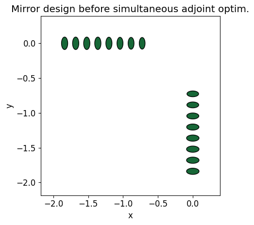
Initial Design Parameters
N_wgx_params = len(initial_border_params)
N_mirror_params = len(initial_mirror_params)
initial_params = anp.concatenate((initial_border_params, initial_mirror_params))
Plot the polyslabs all together so we can check that they overlap.
ax = right_wg_box.plot(z=0)
top_wg_box.plot(z=0, ax=ax)
left_wg_box.plot(z=0, ax=ax)
bot_wg_box.plot(z=0, ax=ax)
wgx_polyslab.plot(z=0, ax=ax)
mirror_struct.plot(z=0, ax=ax)

ax.set_xlim([-3, 3])
ax.set_ylim([-3, 3])
ax.set_title("Design before simultaneous adjoint optim.")
plt.show()
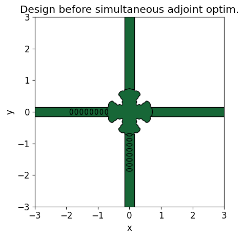
make_sim Function
def split_params(params):
    # Separate the parameters into WGX-related and mirror-related.
    border_params = params[0:N_wgx_params]
    mirror_params = params[N_wgx_params:]
    return border_params, mirror_params


def make_sim(
    params,
    use_fld_mnt: bool = True,
) -> td.Simulation:
    border_params, mirror_params = split_params(params)

    # Structures
    wgx_struct = make_wgx_structure(border_params, smidge, num_vertices)
    two_mirrors_struct = make_2_mirrors_struct_2(mirror_params)
    structures = static_structures + [wgx_struct, two_mirrors_struct]

    # Sources and monitors
    sources = [dipole_src]
    monitors = [right_monitor, top_monitor] + box_monitors

    if use_fld_mnt == True:
        monitors = monitors + [field_monitor_xy]

    # Simulation size is the bounding box of the geometry modified by some multiple of pml_spacing.
    pml_spacing = 0.5
    sim_size = (
        1.0 * wg_length + cross_width - 1 * pml_spacing,
        1.0 * wg_length + cross_width - 1 * pml_spacing,
        wg_height + 2 * pml_spacing,
    )
    sim_origin = (
        -0.2 * wg_length,
        -0.2 * wg_length,
        0,
    )  # displaced to the left and down somewhat

    # Initialize simulation
    sim = td.Simulation(
        structures=structures,
        sources=sources,
        monitors=monitors,
        size=sim_size,
        center=sim_origin,
        grid_spec=grid_spec,
        run_time=run_time,
        boundary_spec=boundary_spec,
        symmetry=symmetry_B,
    )
    return sim


sim = make_sim(params=initial_params, use_fld_mnt=False)

fig, (ax1, ax2) = plt.subplots(1, 2, figsize=(10, 4), tight_layout=True)
sim.plot(z=0, ax=ax1)
ax1.set_title("Initial design, top view")
sim.plot(x=0, ax=ax2)
ax2.set_title("Initial design, side view at x=0")
plt.show()
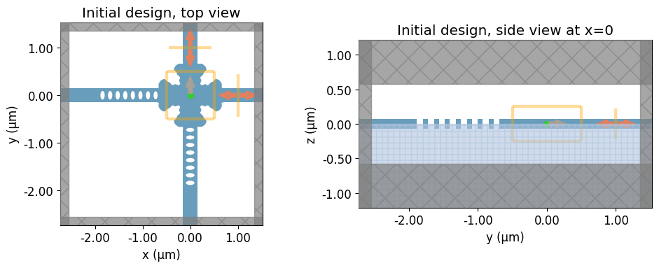
Redefine Some Penalties and Wrapper
In Stage 4, we must redefine the penalty wrapper function because the parameterization is different from Stage 2. We need to separate the WGX parameters from the mirror parameters, and account for the reduced symmetry in the WGX.
Control-Space Smoothness Penalty
def control_space_smoothness(wgx_params, eps=1e-3):
    """
    wgx_params: 1D array of design parameters.

    Returns:
        Scalar smoothness penalty based on turning angles
        of the full polygonal chain
    """

    def calc_penalty(ctrl):
        M = ctrl.shape[0]
        if M < 3:
            return anp.array(0.0)
        # Segments
        seg = ctrl[1:] - ctrl[:-1]  # (M-1,2)
        seg_len = anp.sqrt(anp.sum(seg**2, axis=1)) + eps
        u = seg / seg_len[:, None]  # unit directions
        # Turning angles via dot products
        dot = anp.sum(u[1:] * u[:-1], axis=1)  # (M-2,)
        dot = anp.clip(dot, -1.0, 1.0)
        # Bending measure
        bending = 1.0 - dot  # ~theta^2/2 for small angles
        penalty = anp.sum(bending**2)
        return penalty

    penalty = 0
    for quad in [1, 2, 3, 4]:
        ctrl = quadrant_ctrl_pts_from(
            border_params=wgx_params, quad=quad, smidge=smidge
        )
        penalty = penalty + calc_penalty(ctrl)

    return penalty
Control Point Spacing Penalty
def control_point_spacing_penalty(wgx_params, s_min=0.005, eps=1e-12):
    """
    Penalize neighboring control points getting too close.

    wgx_params: 1D array of design parameters.

    s_min: float
        Desired minimum segment length (same units as coordinates).

    eps: float
        Small amount to avoid a divide-by-zero error

    Returns:
        Scalar spacing penalty. Large when some segments are shorter than s_min.
    """

    def calc_penalty(ctrl):
        # Segment lengths
        seg = ctrl[1:] - ctrl[:-1]  # (M-1,2)
        seg_len = anp.sqrt(anp.sum(seg**2, axis=1)) + eps  # (M-1,)

        # Soft penalty for segments shorter than s_min
        # softplus(z) ~ max(0, z) but smooth
        def softplus(z):
            return anp.log1p(anp.exp(z))

        z = (s_min - seg_len) / (s_min + eps)  # dimensionless
        # Only positive z (seg_len < s_min) contribute significantly
        penalty = anp.sum(softplus(z) ** 2)
        return penalty

    penalty = 0
    for quad in [1, 2, 3, 4]:
        ctrl = quadrant_ctrl_pts_from(
            border_params=wgx_params, quad=quad, smidge=smidge
        )
        penalty = penalty + calc_penalty(ctrl)
    penalty = penalty / 4  # so it's more like the value for one quadrant from before

    return penalty
Penalty Wrapper Function
def eval_penalties(params):
    """Evaluate all the penalties on a set of params."""
    wgx_params, _ = split_params(params)

    border_vertices = all_vertices_from(wgx_params, smidge, num_vertices)

    curve_pen = curve_penalty(border_vertices)

    min_sep_pen = min_separation_penalty(
        border_vertices, vert_d_min=vert_d_min, alpha=alpha, eps=eps, skip=skip
    )

    smoothness_pen = control_space_smoothness(wgx_params)

    spacing_pen = control_point_spacing_penalty(wgx_params, ctrl_s_min)

    border_dist_pen = vertices_dist_penalty(border_vertices, border_d_min, curve_range)

    return (curve_pen, min_sep_pen, smoothness_pen, spacing_pen, border_dist_pen)


eval_penalties(initial_params)
(np.float64(0.5269680305769388),
 np.float64(4.876201949650504e-05),
 np.float64(6.145317090882038),
 np.float64(6.963831897798998),
 np.float64(0.0077892070576361366))
Objective Definition
# We can make a variable that `objective` can modify in place even when called inside `value_and_grad`.
# Then we can access that after running `value_and_grad`
sim_data_last = [None]

# Brief description of the objective formula
obj_descr = "coupling - crosstalk - five penalties, no Purcell included"

# Weights for dipole source. CHANGE THE obj_descr IF YOU CHANGE THE WEIGHTS.
purcell_target = 1
weight_purcell = 0
weight_coupling = 1
weight_brightness = (
    0  # Brightness is the product of Purcell factor and coupling efficiency.
)
weight_cross_dipole = 5

# Weights for penalties. CHANGE THE obj_descr IF YOU CHANGE THE WEIGHTS.
weight_curve_pen = 0.01
weight_minsep_pen = 0.3
weight_smooth = 0.03
weight_spacing = 0.01
weight_border_dist = 0.01


def objective(
    params: anp.ndarray, use_fld_mnt: bool = False, verbose: bool = False
) -> float:
    sim = make_sim(params=params, use_fld_mnt=use_fld_mnt)
    sim_data = web.run(
        sim, task_name="wgx_border_mirror_simul_adjoint", verbose=verbose
    )
    sim_data_last[0] = sim_data

    purcell, coupling, brightness, crosstalk = dipole_figs_of_merit(sim_data)
    wgx_params, _ = split_params(params)
    curve_pen, min_sep_pen, smoothness_pen, spacing_pen, border_dist_pen = (
        eval_penalties(wgx_params)
    )
    obj = (
        -((purcell_target - purcell[center_idx]) ** 2) * weight_purcell
        + coupling[center_idx] * weight_coupling
        + brightness[center_idx] * weight_brightness
        - crosstalk[center_idx] * weight_cross_dipole
        - curve_pen * weight_curve_pen
        - min_sep_pen * weight_minsep_pen
        - smoothness_pen * weight_smooth
        - spacing_pen * weight_spacing
        - border_dist_pen * weight_border_dist
    )
    return obj, [
        purcell,
        coupling,
        brightness,
        crosstalk,
        curve_pen,
        min_sep_pen,
        smoothness_pen,
        spacing_pen,
        border_dist_pen,
    ]


min_or_max = -1  # 1=minimize the objective; -1=maximize the objective
Optional Test
We can test out the calculation of the objective function and figures of merit.
# Took about a minute.
obj, foms = objective(params=initial_params, use_fld_mnt=True, verbose=True)
09:36:47 Eastern Daylight Time Created task 'wgx_border_mirror_simul_adjoint'
                               with resource_id
                               'fdve-dbedfa89-24b4-47e5-9796-5badca14abe6' and
                               task_type 'FDTD'.
                               View task using web UI at
                               'https://tidy3d.simulation.cloud/workbench?taskId
                               =fdve-dbedfa89-24b4-47e5-9796-5badca14abe6'.
Task folder: 'default'.
Output()
09:36:54 Eastern Daylight Time Estimated FlexCredit cost: 0.042. Minimum cost
                               depends on task execution details. Use
                               'web.real_cost(task_id)' to get the billed
                               FlexCredit cost after a simulation run.
09:36:55 Eastern Daylight Time status = queued
                               To cancel the simulation, use
                               'web.abort(task_id)' or 'web.delete(task_id)' or
                               abort/delete the task in the web UI. Terminating
                               the Python script will not stop the job running
                               on the cloud.
Output()
09:37:05 Eastern Daylight Time starting up solver
running solver
Output()
09:37:13 Eastern Daylight Time early shutoff detected at 72%, exiting.
status = postprocess
Output()
09:37:20 Eastern Daylight Time status = success
09:37:22 Eastern Daylight Time View simulation result at
                               'https://tidy3d.simulation.cloud/workbench?taskId
                               =fdve-dbedfa89-24b4-47e5-9796-5badca14abe6'.
Output()
09:37:44 Eastern Daylight Time Loading simulation from simulation_data.hdf5
Adjoint Gradient
val_grad = value_and_grad(objective, has_aux=True)
Optional Test
# This takes about 5 minutes to run.
(val, grad), foms = val_grad(initial_params, use_fld_mnt=False, verbose=True)
09:37:52 Eastern Daylight Time Created task 'wgx_border_mirror_simul_adjoint'
                               with resource_id
                               'fdve-ff183c85-b855-4f8f-8b4f-e07b43d5bb29' and
                               task_type 'FDTD'.
                               View task using web UI at
                               'https://tidy3d.simulation.cloud/workbench?taskId
                               =fdve-ff183c85-b855-4f8f-8b4f-e07b43d5bb29'.
Task folder: 'default'.
Output()
09:37:58 Eastern Daylight Time Estimated FlexCredit cost: 0.042. Minimum cost
                               depends on task execution details. Use
                               'web.real_cost(task_id)' to get the billed
                               FlexCredit cost after a simulation run.
Output()
09:38:03 Eastern Daylight Time status = queued
                               To cancel the simulation, use
                               'web.abort(task_id)' or 'web.delete(task_id)' or
                               abort/delete the task in the web UI. Terminating
                               the Python script will not stop the job running
                               on the cloud.
Output()
09:38:14 Eastern Daylight Time starting up solver
running solver
Output()
09:38:33 Eastern Daylight Time early shutoff detected at 72%, exiting.
status = postprocess
Output()
09:38:52 Eastern Daylight Time status = success
09:38:54 Eastern Daylight Time View simulation result at
                               'https://tidy3d.simulation.cloud/workbench?taskId
                               =fdve-ff183c85-b855-4f8f-8b4f-e07b43d5bb29'.
Output()
09:39:05 Eastern Daylight Time Loading simulation from
                               simulation_data_adjoint.hdf5
09:41:13 Eastern Daylight Time Started working on Batch containing 1 tasks.
09:41:26 Eastern Daylight Time Maximum FlexCredit cost: 0.033 for the whole
                               batch.
                               Use 'Batch.real_cost()' to get the billed
                               FlexCredit cost after completion.
Output()
09:42:32 Eastern Daylight Time Batch complete.
Output()
Hyperparameters, Metadata, and History
# Hyperparameters for optimization routine
num_steps = 50
learning_rate = 0.005

# Initialize adam optimizer with the starting parameters
optimizer = optax.adam(learning_rate=learning_rate)
opt_state = optimizer.init(initial_params)

# Directory and file in which to store optimization history
simul_adoint_run_title = "wgx_border_mirror_simul_adjoint"
history_name = f"{simul_adoint_run_title}_{run_number:02d}.pkl"
history_dir = Path("misc")
history_dir.mkdir(parents=True, exist_ok=True)
history_file_4 = history_dir / history_name

# Metadata associated with the optimization and simulation setup
simul_adjoint_metadata = dict(
    # Source
    center_wavelength=wl,
    bandwidth=bw,
    # Material
    index=n_AlGaAs,
    wg_height=wg_height,
    wg_width=wg_width,
    # Waveguide crossing
    cross_width=cross_width,
    smidge=smidge,
    num_free_pts=num_free_pts,
    num_vertices=num_vertices,
    # Penalty parameters
    min_curv_radius=min_curv_radius,
    penalty_alpha=alpha,
    penalty_kappa=kappa,
    min_vertex_sep=vert_d_min,
    penalty_eps=eps,
    skip=skip,
    ctrl_s_min=ctrl_s_min,
    border_d_min=border_d_min,
    curve_range=curve_range,
    # Mirror
    num_holes=num_holes,
    dipole_mirror_dist_span=dipole_mirror_dist_span,
    hole_x_width_span=hole_x_width_span,
    hole_y_width_span=hole_y_width_span,
    bridge_width_span=bridge_width_span,
    # Objective weights
    obj_descr=obj_descr,
    weight_purcell=weight_purcell,
    weight_coupling=weight_coupling,
    weight_brightness=weight_brightness,
    weight_cross=weight_cross_dipole,
    weight_curve_pen=weight_curve_pen,
    weight_minsep_pen=weight_minsep_pen,
    weight_smooth=weight_smooth,
    weight_spacing=weight_spacing,
    weight_border_dist=weight_border_dist,
    # Optimizer hyperparameters
    num_steps=num_steps,
    learning_rate=learning_rate,
    pickle_file=history_name,
)
Check for a previous optimization and load it if it exists.
try:  # to load a previous optimization
    history_dict_4 = load_history(history_file_4)
    opt_state = history_dict_4["opt_states"][-1]
    params = history_dict_4["params"][-1].copy()
    num_steps_completed = len(history_dict_4["values"])
    simul_adjoint_metadata = history_dict_4["simul_adjoint_metadata"]
    print("Loaded optimization checkpoint from file.")
    print(f"Found {num_steps_completed} iterations previously completed.")

except FileNotFoundError:  # Initialize a new optimization
    print("No previous checkpoint file found. Initializing a new optimization.")
    params = initial_params.copy()
    opt_state = optimizer.init(params)
    history_dict_4 = dict(
        values=[],
        purcell=[],
        coupling=[],
        brightness=[],
        crosstalk=[],
        curve_pen=[],
        min_sep_pen=[],
        smoothness_pen=[],
        spacing_pen=[],
        border_dist_pen=[],
        params=[params.copy()],
        gradients=[],
        opt_states=[opt_state],
        simul_adjoint_metadata=simul_adjoint_metadata,
    )
No previous checkpoint file found. Initializing a new optimization.
Uncomment and run the cell below if you want to truncate the history so the optimization starts at iteration start_iter.
# start_iter = 3

# total_iter = len(history_dict_4['values'])
# if start_iter is not None and start_iter < total_iter:
#     print(f'Iterations in history: {total_iter}')
#     print(f'Starting at iteration {start_iter}')
#     for key in history_dict_4.keys():
#         if key in set(['params', 'opt_states', 'simul_adjoint_metadata']):
#             continue
#         history_dict_4[key] = history_dict_4[key][:start_iter]
#     history_dict_4['params'] = history_dict_4['params'][:start_iter+1]
#     history_dict_4['opt_states'] = history_dict_4['opt_states'][:start_iter+1]
#     simul_adjoint_metadata['num_steps'] = start_iter
#     history_dict_4['simul_adjoint_metadata']['num_steps'] = start_iter

#     opt_state = history_dict_4['opt_states'][-1]
#     params = history_dict_4['params'][-1].copy()
#     num_steps_completed = len(history_dict_4['values'])
# else:
#     print(f'Iterations in history ({total_iter}) already less than or equal to start_iter ({start_iter})')
Uncomment and run the cell below if there is an existing previous optimization but you don't want to load it.
# params = initial_params.copy()
# opt_state = optimizer.init(params)
# history_dict_4 = dict(
#     values = [],
#     purcell = [],
#     coupling = [],
#     brightness = [],
#     crosstalk = [],
#     curve_pen = [],
#     min_sep_pen = [],
#     smoothness_pen = [],
#     spacing_pen = [],
#     border_dist_pen = [],
#     params = [params.copy()],
#     gradients = [],
#     opt_states = [opt_state],
#     simul_adjoint_metadata = simul_adjoint_metadata,
# )
Estimated Cost
# initializes job, puts task on server (but doesnt run it)
job = web.Job(simulation=sim, task_name="cost_estimate", verbose=False)

# estimate the maximum cost
est_cost_per_sim = web.estimate_cost(job.task_id)
cost_estimate = est_cost_per_sim * num_steps * 2  # for the adjoint sims

print(
    f"The estimated maximum cost is {cost_estimate:.3f} Flex Credits for {num_steps} iterations of adjoint optimization."
)
09:43:19 Eastern Daylight Time Estimated FlexCredit cost: 0.042. Minimum cost
                               depends on task execution details. Use
                               'web.real_cost(task_id)' to get the billed
                               FlexCredit cost after a simulation run.
The estimated maximum cost is 4.187 Flex Credits for 50 iterations of adjoint optimization.
Run the Optimization
In each iteration, calculate the objective value and gradient then update the parameters and optimizer state. Note that in the end, history_dict will have one more element of params and opt_states than it does of values and gradients.
# Took 4:48 hours for 50 iterations and cost about 4 flexcredits.

td.config.logging_level = (
    "ERROR"  # Only give errors and ignore warnings to reduce clutter.
)

for i in tqdm(range(num_steps)):
    # Compute gradient and current objective function value
    (value, gradient), foms = val_grad(params)

    # Get the values of the individual figures of merit (foms)
    (
        purcell,
        coupling,
        brightness,
        crosstalk,
        curve_pen,
        min_sep_pen,
        smoothness_pen,
        spacing_pen,
        border_dist_pen,
    ) = [out._value for out in foms]

    # Compute and apply updates to the optimizer based on gradient
    updates, opt_state = optimizer.update(min_or_max * gradient, opt_state, params)
    params[:] = optax.apply_updates(params, updates)

    # save history
    history_dict_4["values"].append(value)
    history_dict_4["crosstalk"].append(crosstalk)
    history_dict_4["purcell"].append(purcell)
    history_dict_4["coupling"].append(coupling)
    history_dict_4["brightness"].append(brightness)
    history_dict_4["curve_pen"].append(curve_pen)
    history_dict_4["min_sep_pen"].append(min_sep_pen)
    history_dict_4["smoothness_pen"].append(smoothness_pen)
    history_dict_4["spacing_pen"].append(spacing_pen)
    history_dict_4["border_dist_pen"].append(border_dist_pen)
    history_dict_4["params"].append(
        params.copy()
    )  # Need to .copy otherwise all parameter sets are the same.
    history_dict_4["gradients"].append(gradient)
    history_dict_4["opt_states"].append(opt_state)
    save_history(history_dict_4, history_file_4)

simul_adjoint_metadata["num_steps"] = len(history_dict_4["values"])
history_dict_4["metadata"] = simul_adjoint_metadata
0%| | 0/50 [00:00<?, ?it/s]
Confirm the Actual Cost
# For an adoint optimization, num_tasks is:
num_tasks = num_steps * 2  # for the adjoint sims

# Get the task information for the last num_tasks simulations.
task_dict_list = web.api.webapi.get_tasks(num_tasks)
cost_array = []
for task_dict in task_dict_list:
    cost_array.append(
        task_dict["realFlexUnit"]
    )  # The real cost is contained in the task dictionary
cost_array = anp.array(cost_array)
total_cost = anp.cumsum(cost_array)[-1]  # Sum the costs of all the simulations

# Might as well save the task information, too.
history_dict_4["task_dict_list"] = task_dict_list
save_history(history_dict_4, history_file_4)

print(f"Total cost of the optimization run: {total_cost:.4f} flexcredits")
print(f"Estimated cost: {cost_estimate:.3f} flexcredits")
print(f"Fraction of estimated cost: {total_cost / cost_estimate:.3f}")
Total cost of the optimization run: 3.1586 flexcredits
Estimated cost: 4.187 flexcredits
Fraction of estimated cost: 0.754
Analyzing Optimization Results
After the optimization is finished, let's look at the results.
Metadata
simul_adjoint_metadata["num_steps"] = len(history_dict_4["values"])
history_dict_4["metadata"] = simul_adjoint_metadata

simul_adjoint_metadata
{'center_wavelength': 0.798,
 'bandwidth': 0.02,
 'index': np.float64(3.5693094750241627),
 'wg_height': 0.15,
 'wg_width': 0.3,
 'cross_width': 1.4,
 'smidge': 0.02,
 'num_free_pts': 30,
 'num_vertices': 600,
 'min_curv_radius': 0.1,
 'penalty_alpha': 1.0,
 'penalty_kappa': 5.0,
 'min_vertex_sep': 0.3,
 'penalty_eps': 0.001,
 'skip': 20,
 'ctrl_s_min': 0.01,
 'border_d_min': 0.3,
 'curve_range': 0.01,
 'num_holes': 8,
 'dipole_mirror_dist_span': (0.3, 1.5),
 'hole_x_width_span': (0.068, 0.5),
 'hole_y_width_span': (0.1, 0.185),
 'bridge_width_span': (0.068, 0.5),
 'obj_descr': 'coupling - crosstalk - five penalties, no Purcell included',
 'weight_purcell': 0,
 'weight_coupling': 1,
 'weight_brightness': 0,
 'weight_cross': 5,
 'weight_curve_pen': 0.01,
 'weight_minsep_pen': 0.3,
 'weight_smooth': 0.03,
 'weight_spacing': 0.01,
 'weight_border_dist': 0.01,
 'num_steps': 50,
 'learning_rate': 0.005,
 'pickle_file': 'wgx_border_mirror_simul_adjoint_20.pkl'}
Objective Evolution
fig, ax = plt.subplots(1, 1, figsize=(6, 4))
ax.plot(history_dict_4["values"], ".-")
ax.set_xlabel("Iteration number")
ax.set_ylabel("Objective function")
ax.set_title("Optimization progress")
plt.show()
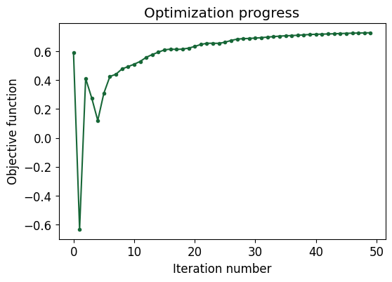
Plot the objective and the weighted contributions from each figure of merit and penalty.
# For a dipole source.

fig, ax = plt.subplots(1, 1, figsize=(8, 4))

purcell_w = (
    purcell_target - anp.array(history_dict_4["purcell"])[:, center_idx]
) ** 2 * weight_purcell
coupling_w = anp.array(history_dict_4["coupling"])[:, center_idx] * weight_coupling
brightness_w = (
    anp.array(history_dict_4["brightness"])[:, center_idx] * weight_brightness
)
cross_w = -anp.array(history_dict_4["crosstalk"])[:, center_idx] * weight_cross_dipole
curve_pen_w = -anp.array(history_dict_4["curve_pen"]) * weight_curve_pen
minsep_pen_w = -anp.array(history_dict_4["min_sep_pen"]) * weight_minsep_pen
smooth_pen_w = -anp.array(history_dict_4["smoothness_pen"]) * weight_smooth
spacing_pen_w = -anp.array(history_dict_4["spacing_pen"]) * weight_spacing
border_dist_w = -anp.array(history_dict_4["border_dist_pen"]) * weight_border_dist

ax.plot(history_dict_4["values"], ".-", label="Objective")
ax.plot(purcell_w, ".-", label="Purcell (not included)")
ax.plot(coupling_w, ".-", label="Coupling")
ax.plot(brightness_w, ".-", label="Brightness")
ax.plot(cross_w, ".-", label="Crosstalk")
ax.plot(curve_pen_w, ".-", label="Curvature penalty")
ax.plot(minsep_pen_w, ".-", label="Min sep penalty")
ax.plot(smooth_pen_w, ".-", label="Smoothness penalty")
ax.plot(spacing_pen_w, ".-", label="Spacing penalty")
ax.plot(border_dist_w, ".-", label="Border dist penalty")
ax.set_xlabel("Iteration number")
ax.set_ylabel("Contributions to objective")
ax.set_title("Objective function and contributions")

# Position legend to the right of the plot
ax.legend(loc="upper left", bbox_to_anchor=(1.05, 1))
# Adjust layout to prevent cutting off the legend
plt.tight_layout()
plt.show()
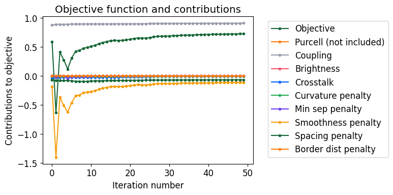
Figures of Merit Evolution
# For the dipole source version

fig, (ax1, ax2, ax3) = plt.subplots(1, 3, figsize=(10, 4), tight_layout=True)

ax1.plot(
    anp.array(history_dict_4["purcell"])[:, center_idx], ".-", label="Purcell factor"
)
ax1.plot(anp.array(history_dict_4["coupling"])[:, center_idx], ".-", label="Coupling")
ax1.plot(
    anp.array(history_dict_4["brightness"])[:, center_idx], ".-", label="Brightness"
)
ax1.legend()
ax1.set_xlabel("Iteration number")

ax2.plot(anp.array(history_dict_4["crosstalk"])[:, center_idx], ".-", label="Crosstalk")
ax2.set_xlabel("Iteration number")
ax2.legend()
# ax2.set_ylabel('Crosstalk')

ax3.plot(history_dict_4["curve_pen"], ".-", label="Curvature penalty")
ax3.plot(history_dict_4["min_sep_pen"], ".-", label="Min sep penalty")
ax3.plot(history_dict_4["smoothness_pen"], ".-", label="Smoothness pen")
ax3.plot(history_dict_4["spacing_pen"], ".-", label="Spacing pen")
ax3.plot(history_dict_4["border_dist_pen"], ".-", label="Border dist pen")
ax3.legend()
ax3.set_xlabel("Iteration number")

plt.show()
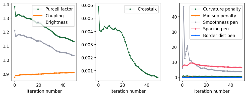
The coupling efficiency has increased slightly, while the Purcell factor and brightness have decreased. The crosstalk declined even further than it did in Stage 2, now it is less than 1 part in a thousand at the design wavelength.
Final figures of merit.
print(f"Final figures of merit at {wl * 1e3} nm:")
print(f"\tPurcell factor:\t{history_dict_4['purcell'][-1][center_idx]:.3f}")
print(f"\tCoupling:\t{100 * history_dict_4['coupling'][-1][center_idx]:.2f} %")
print(f"\tBrightness:\t{history_dict_4['brightness'][-1][center_idx]:.3f}")
print(f"\tCrosstalk:\t{100 * history_dict_4['crosstalk'][-1][center_idx]:.5f} %")
Final figures of merit at 798.0 nm:
	Purcell factor:	1.132
	Coupling:	91.07 %
	Brightness:	1.031
	Crosstalk:	0.04987 %
The coupling increased slightly from 88% to 91% while the crosstalk decreased by an order of magnitude from 0.6% to 0.05%. These improvements came at the cost of the Purcell factor--and thus brightness--decreasing somewhat.
Figures of Merit Spectra
Plot the FOM spectra of the final design.
# For the dipole source version.

fig, (ax1, ax2, ax3) = plt.subplots(1, 3, figsize=(10, 4), tight_layout=True)

ax1.plot(
    wl_range * 1000,
    anp.array(history_dict_4["purcell"])[-1, :],
    ".-",
    label="Purcell factor",
)
ax1.plot(
    wl_range * 1000,
    anp.array(history_dict_4["brightness"])[-1, :],
    ".-",
    label="Brightness",
)
ax1.legend()
ax1.set_xlabel("Wavelength (nm)")

ax2.plot(
    wl_range * 1000,
    anp.array(history_dict_4["coupling"])[-1, :],
    ".-",
    label="Coupling",
)
ax2.set_xlabel("Wavelength (nm)")
ax2.legend()

ax3.plot(
    wl_range * 1000,
    anp.array(history_dict_4["crosstalk"])[-1, :],
    ".-",
    label="Crosstalk",
)
ax3.set_xlabel("Wavelength (nm)")
ax3.legend()

plt.show()
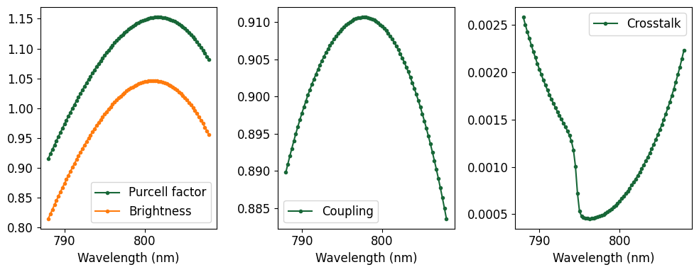
As desired, the extrema of the figures of merit are still located at or near the design wavelength.
Figures of Merit Spectra Evolution
Plot the figures of merit as colormaps versus wavelength and iteration number.
# For the dipole source version.

purcell = anp.array(history_dict_4["purcell"])
coupling = anp.array(history_dict_4["coupling"])
brightness = anp.array(history_dict_4["brightness"])
crosstalk = anp.array(history_dict_4["crosstalk"])
wavelength, iteration = anp.meshgrid(
    wl_range * 1000, [j for j in range(len(purcell))], indexing="xy"
)

fig, axes = plt.subplots(1, 4, figsize=(12, 4))
quantities = [purcell, coupling, brightness, crosstalk]
titles = ["Purcell factor", "Coupling", "Brightness", "Crosstalk"]

for ax, quantity, title in zip(axes, quantities, titles):
    p = ax.pcolormesh(wavelength, iteration, quantity)  # , cmap="plasma")
    ax.set_xlabel("Wavelength (nm)")
    # ax.set_ylabel('Iteration number')
    ax.set_title(title)
    plt.colorbar(p, ax=ax)
axes[0].set_ylabel("Iteration number")

plt.tight_layout()
plt.show()
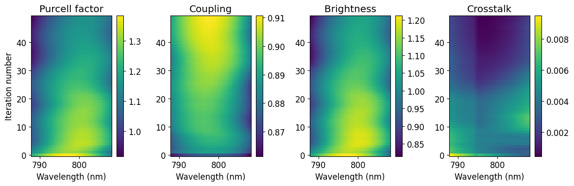
Close-up of Border
initial_wgx_params, initial_mirror_params = split_params(initial_params)
final_wgx_params, final_mirror_params = split_params(history_dict_4["params"][-1])
fig, axes = plt.subplots(2, 2, figsize=(8, 8), tight_layout=True)
axes = [
    axes[0, 1],
    axes[0, 0],
    axes[1, 0],
    axes[1, 1],
]  # rearrange to be ordered like quadrants
control_pts_list = []
vertices_list = []
for quad, ax in zip([1, 2, 3, 4], axes):
    initial_ctrl_pts = quadrant_ctrl_pts_from(initial_wgx_params, quad, smidge)
    initial_vertices = quadrant_vertices_from(
        initial_wgx_params, quad, smidge, num_vertices
    )
    final_ctrl_pts = quadrant_ctrl_pts_from(final_wgx_params, quad, smidge)
    final_vertices = quadrant_vertices_from(
        final_wgx_params, quad, smidge, num_vertices
    )
    control_pts_list.append(final_ctrl_pts)
    vertices_list.append(final_vertices)
    ax.plot(*initial_ctrl_pts.T, ".")
    ax.plot(*initial_vertices.T, "-")
    ax.plot(*final_ctrl_pts.T, ".")
    ax.plot(*final_vertices.T, "-")
    ax.set_aspect("equal")
    ax.set_xlabel("X (um)")
    ax.set_ylabel("Y (um)")
plt.show()
# print(metadata)
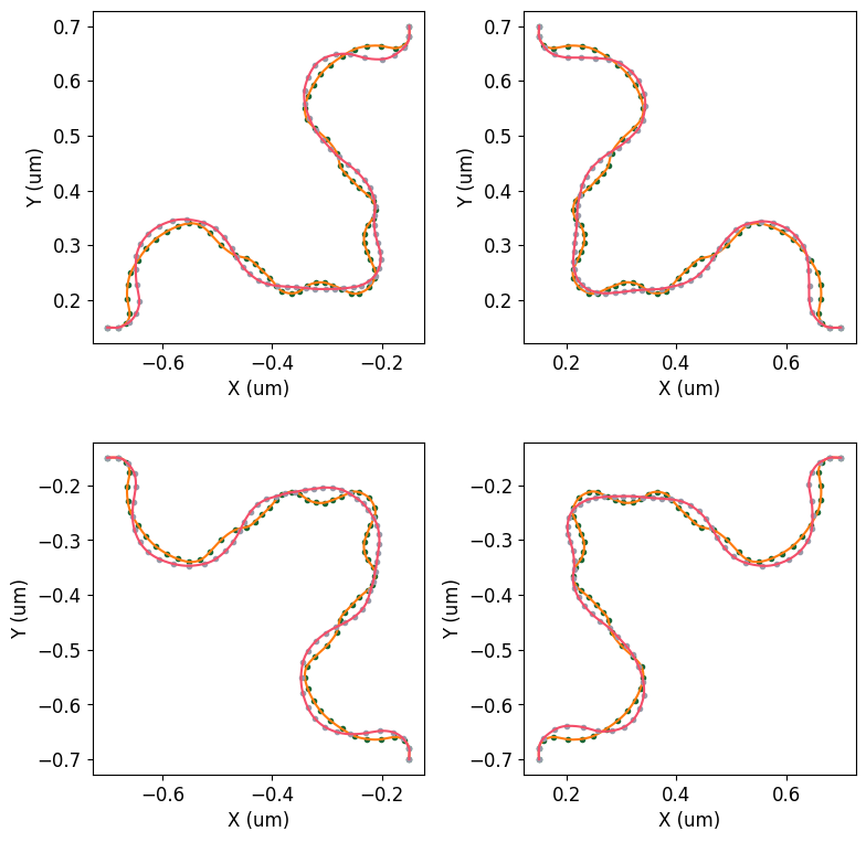
We can see that the final design is different from the initial design, but it's not by a lot. The main difference is that the indentation along the diagonal has fewer wiggles. Close inspection also shows that the four quadrants of the WGX are not all the same anymore, which was allowed by the reduced symmetry of the situation in Stage 4.
# Detect self-intersection
wgx_vertices = all_vertices_from(final_wgx_params)
polyline = LineString(coordinates=wgx_vertices)
polyline.is_simple  # False if there is an intersection
True
Final Mirror Structure Parameters
(
    final_qd_mirror_dist,
    final_hole_x_widths,
    final_hole_y_widths,
    final_bridge_widths,
) = structure_params_from(final_mirror_params)
print(f"QD-to-mirror distance:\t{final_qd_mirror_dist[0]:.3f} microns")
print("Hole x-widths (microns):")  #:\t{hole_x_widths:.3f}')
print(final_hole_x_widths)
print("Hole y-widths (microns):")
print(final_hole_y_widths)
print("Bridge widths (microns):")
print(final_bridge_widths)
QD-to-mirror distance:	0.696 microns
Hole x-widths (microns):
[0.08097659 0.08255415 0.08917321 0.09254519 0.0946468  0.09491131
 0.0951526  0.09533461]
Hole y-widths (microns):
[0.17030474 0.16917564 0.17205974 0.17784112 0.17812112 0.17901319
 0.18075722 0.17892073]
Bridge widths (microns):
[0.07317035 0.07271131 0.07210582 0.07047812 0.06938495 0.06919074
 0.06919959]
(
    initial_qd_mirror_dist,
    initial_hole_x_widths,
    initial_hole_y_widths,
    initial_bridge_widths,
) = structure_params_from(initial_mirror_params)

pct_qd_mirror_dist = (
    100 * (final_qd_mirror_dist - initial_qd_mirror_dist) / initial_qd_mirror_dist
)[0]
pct_hole_x_widths = (
    100 * (final_hole_x_widths - initial_hole_x_widths) / initial_hole_x_widths
)
pct_hole_y_widths = (
    100 * (final_hole_y_widths - initial_hole_y_widths) / initial_hole_y_widths
)
pct_bridge_widths = (
    100 * (final_bridge_widths - initial_bridge_widths) / initial_bridge_widths
)

print(
    f"Percentage changes in mirror structure parameters after {simul_adjoint_metadata['num_steps']} iterations"
)
print("---------------------------------------------------------------------")
print(f"QD-to-mirror distance:\t{pct_qd_mirror_dist:.3f}%")
print("Hole x-widths:")
with anp.printoptions(precision=4, suppress=True):
    print(pct_hole_x_widths)
print("Hole y-widths:")
with anp.printoptions(precision=4, suppress=True):
    print(pct_hole_y_widths)
print("Bridge widths:")
with anp.printoptions(precision=4, suppress=True):
    print(pct_bridge_widths)
Percentage changes in mirror structure parameters after 50 iterations
---------------------------------------------------------------------
QD-to-mirror distance:	1.621%
Hole x-widths:
[-3.432  -3.2412  2.7523  4.8674  5.4974  5.4311  5.6991  5.9013]
Hole y-widths:
[ 1.5728 -0.8332 -0.8453  0.785  -0.7048 -0.5482  0.4207 -0.5996]
Bridge widths:
[-1.644  -0.2975  0.8992  0.6857  0.3951  0.3372  0.35  ]
Animation of Optimization
from matplotlib.animation import FuncAnimation, PillowWriter
from IPython.display import HTML


def get_vertices(index):
    wgx_params, _ = split_params(history_dict_4["params"][index])
    vertices = all_vertices_from(wgx_params, smidge, num_vertices)
    return vertices.T


# Set up the figure and axis
fig, ax = plt.subplots(figsize=(4, 4))
(line,) = ax.plot(*get_vertices(0))
ax.set_aspect("equal")


# Animation update function
def update(frame):
    line.set_data(*get_vertices(frame))
    return (line,)


# Build the FuncAnimation
frames = len(history_dict_4["params"])
interval = 50  # in ms
anim = FuncAnimation(fig, update, frames=frames, interval=interval, blit=True)

# Close the figure display here so it doesn’t show twice in notebook
plt.close(fig)

# Export as animated GIF via Pillow.  Required by matplotlib, or do `pip install pillow`.
gif_writer = PillowWriter(fps=5)
filename = f"{simul_adoint_run_title}_{run_number:02d}.gif"
figs_dir = Path("figs")
figs_dir.mkdir(parents=True, exist_ok=True)
fig_file = figs_dir / filename
anim.save(fig_file, writer=gif_writer)
print(f"Saved animation as {filename}")

# Display inline as HTML5 video (JS-based)
HTML(anim.to_jshtml())  # Must be the last line of the cell for it to display properly.
Saved animation as wgx_border_mirror_simul_adjoint_20.gif
Final Crossing Design
initial_cross_polyslab = make_wgx_polyslab(initial_wgx_params, smidge, num_vertices)
final_cross_polyslab = make_wgx_polyslab(final_wgx_params, smidge, num_vertices)
fig, (ax1, ax2) = plt.subplots(1, 2, figsize=(10, 4), tight_layout=True)
initial_cross_polyslab.plot(z=0, ax=ax1)
ax1.set_title("Initial WGX design")
final_cross_polyslab.plot(z=0, ax=ax2)
ax2.set_title("Final WGX design")
plt.show()
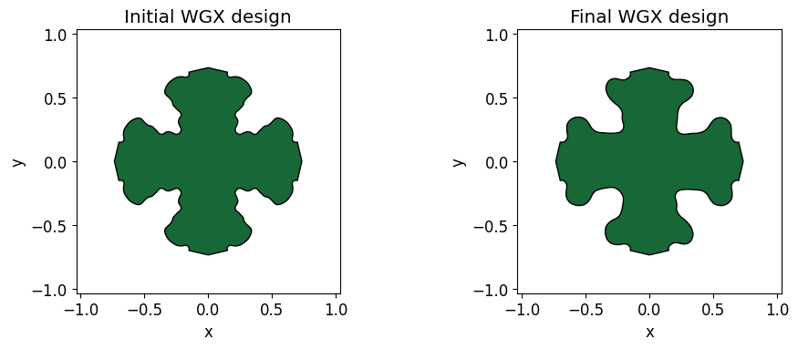
Field in the Final Design
sim_best = make_sim(history_dict_4["params"][-1], use_fld_mnt=True)
fig, ax = plt.subplots()
sim_best.plot(z=0, ax=ax)
plt.show()
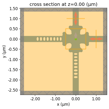
sim_best_data = web.run(
    sim_best, task_name="wgx_border_mirror_simul_adj_best", verbose=False
)
f, ax = plt.subplots()
vminmax = 10000
huh = sim_best_data.plot_field(
    "field_xy", "Ey", ax=ax, vmin=-vminmax, vmax=vminmax, phase=0 * anp.pi
)
ax.set_title("Final adjoint design")
plt.show()
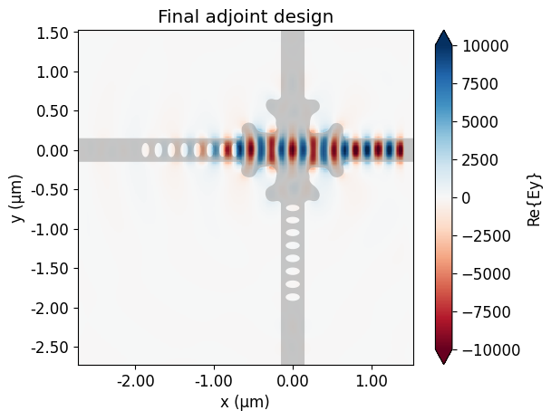
Any crosstalk is now barely visible, while the coupling to the desired output waveguide is strong.
Animation of Field
from matplotlib.animation import FuncAnimation, PillowWriter
from IPython.display import HTML

# Set up the figure and axis
fig, ax = plt.subplots(figsize=(4, 4))

# Plot once to get everything in place
im = sim_best_data.plot_field(
    "field_xy", "Ey", ax=ax, vmin=-vminmax, vmax=vminmax, phase=0 * anp.pi
)
ax.set_title("Final design")
field_artist = im.get_children()[0]  # First child is the field QuadMesh object.

# Get the complex field array.
# Important to use .apply_phase because it interpolates the monitor data in the same way as .plot_field, above.
field_data = sim_best_data["field_xy"]
field_phi = field_data.apply_phase(anp.pi / 4)
Ey_complex = field_phi.Ey.values[:, :, 0, 0].T


# Change the phase of the (real) field
def field_at_phase(phi):
    """Return real part of field at phase phi."""
    return anp.real(Ey_complex * anp.exp(-1j * phi))


# Animation update function
vminmax = 10000
frames = 24
phase_array = anp.arange(frames) * 2 * anp.pi / frames


def update(frame):
    new_data = field_at_phase(phase_array[frame])
    field_artist.set_array(new_data.ravel())
    return (field_artist,)


# Build the FuncAnimation
interval = 50  # in ms
anim = FuncAnimation(fig, update, frames=frames, interval=interval, blit=True)

# Close the figure display here so it doesn’t show twice in notebook
plt.close(fig)

# Export as animated GIF via Pillow.  Required by matplotlib, or do `pip install pillow`.
gif_writer = PillowWriter(fps=5)
filename = f"{simul_adoint_run_title}_{run_number:02d}_field_anim.gif"
figs_dir = Path("figs")
figs_dir.mkdir(parents=True, exist_ok=True)
fig_file = figs_dir / filename
anim.save(fig_file, writer=gif_writer)
print(f"Saved animation as {filename}")

# Display inline as HTML5 video (JS-based)
HTML(anim.to_jshtml())  # Must be the last line of the cell for it to display properly.
Saved animation as wgx_border_mirror_simul_adjoint_20_field_anim.gif
Directional Power Analysis
# Taking the code from the figures of merit function, we can calculate the total power radiated by the dipole.
dipole_power = anp.sum(
    anp.array(
        [anp.abs(sim_best_data[monitor.name].flux.values) for monitor in box_monitors]
    ),
    axis=0,
)
# Its shape is (81,), which is one value for every frequency recorded in the simulation.

box_fluxes = anp.array(
    [anp.abs(sim_best_data[monitor.name].flux.values) for monitor in box_monitors]
)
side_names = ["Left", "Right", "Bottom", "Top", "Lower", "Upper"]
power_fractions = 100 * box_fluxes[:, center_idx] / dipole_power[center_idx]
best_coupling_pct = 100 * history_dict_4["coupling"][-1][center_idx]
best_crosstalk_pct = 100 * history_dict_4["crosstalk"][-1][center_idx]

print("Side\tPower fraction (%)")
print("-------------------------")
for side, fraction in zip(side_names, power_fractions):
    if side == "Right":
        print(
            f"{side}:\t{fraction:.2f}\tCoupling: {best_coupling_pct:.2f}\t\tDifference: {fraction - best_coupling_pct:.2f}"
        )
    elif side == "Bottom" or side == "Top":
        print(
            f"{side}:\t{fraction:.2f}\tCrosstalk: {best_crosstalk_pct:.5f}\tDifference: {fraction - best_crosstalk_pct:.2f}"
        )
    else:
        print(f"{side}:\t{fraction:.2f}")
Side	Power fraction (%)
-------------------------
Left:	1.26
Right:	92.71	Coupling: 91.07		Difference: 1.64
Bottom:	0.78	Crosstalk: 0.04987	Difference: 0.73
Top:	0.54	Crosstalk: 0.04987	Difference: 0.49
Lower:	2.36
Upper:	2.36
The vast majority of power (91%) goes into the output waveguide. Another 1.7% goes in that direction but not confined in the waveguide. Only 1.3% goes to the left. Only 0.5% goes north and 0.8% south, and almost none of it is confined in the top and bottom waveguides. About 4.7% of the power goes out of the plane.


 TERMS & CONDITIONS


 How the process works:
 Try this real URL to see an example: