





Author: Taekyung Kim, Korea Advanced Institute of Science & Technology (KAIST)
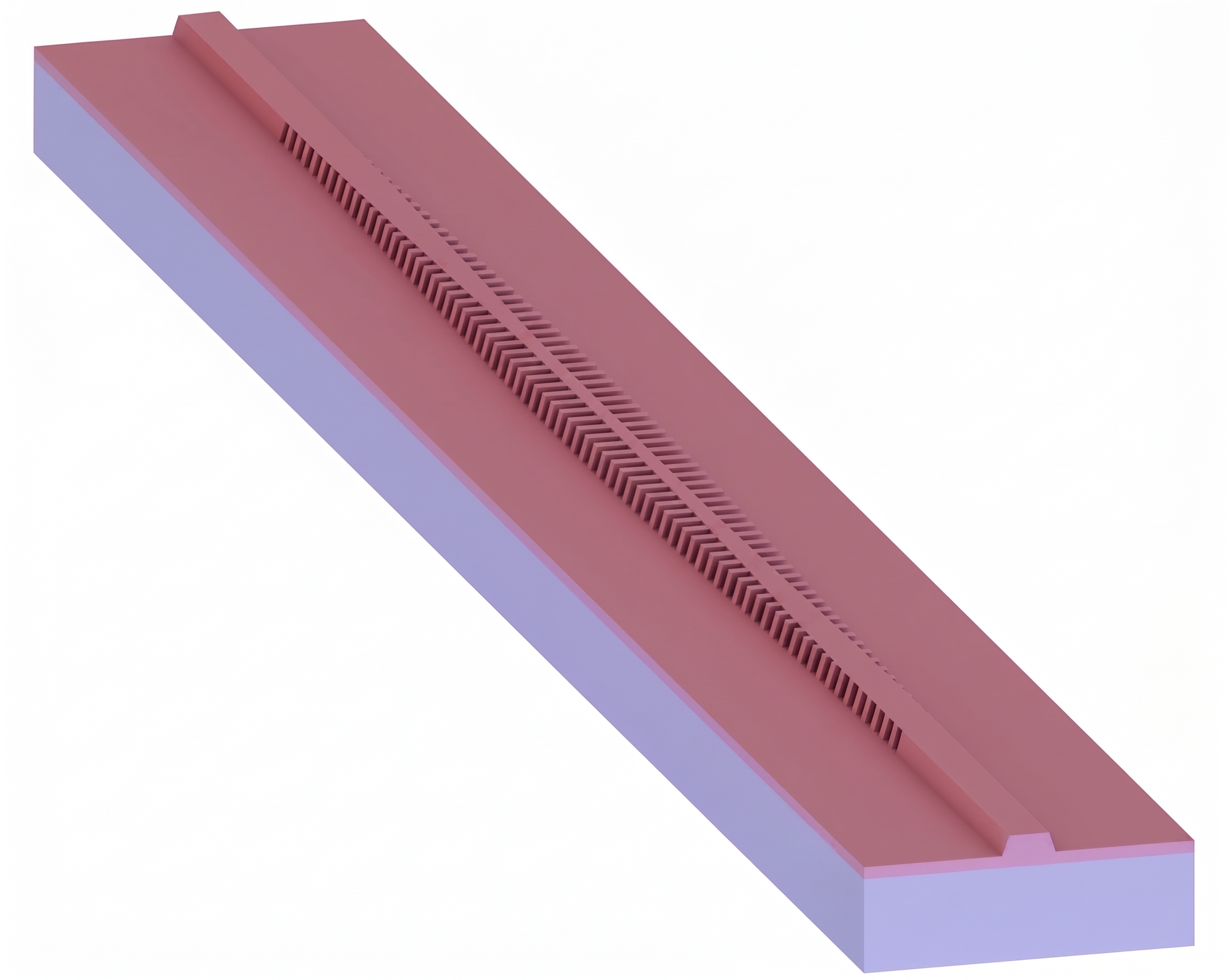
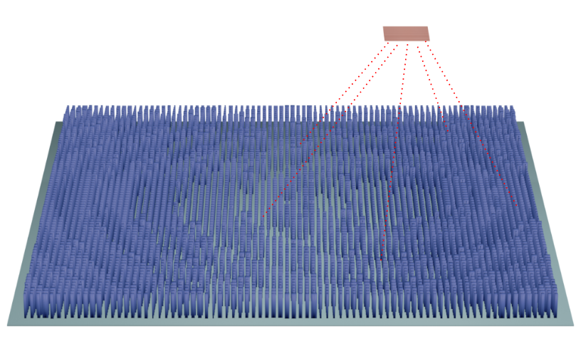
Photonic crystal (PhC) Bragg reflectors use a periodic modulation of a waveguide to couple forward- and backward-propagating modes over a designed spectral range. In thin-film lithium niobate (TFLN), these structures can serve as compact mirrors for Fabry–Pérot microresonators while retaining the electro-optic and nonlinear properties of lithium niobate.
In this notebook, we use Tidy3D to analyze a fishbone-shaped TFLN PhC reflector in three steps: we calculate the Bloch-mode band structure of a periodic unit cell, connect the access-waveguide effective index to the Bragg period, and evaluate reflection and guided-mode leakage in a finite apodized reflector.
Reference: H. Hwang et al., “High-Q photonic crystal Fabry–Pérot micro-resonator in thin-film lithium niobate,” APL Photonics 10, 126103 (2025). DOI: 10.1063/5.0284518.
Setup
import matplotlib.pyplot as plt
import numpy as np
import tidy3d as td
import tidy3d.web as web
from tidy3d.plugins import waveguide
from tidy3d.plugins.resonance import ResonanceFinder
The lithium-niobate optical axis is oriented along the $y$ direction, corresponding to the dominant $E_y$ component of the quasi-TE mode considered here.
silica = td.material_library["SiO2"]["Palik_NoLoss"]
ln = td.material_library["LiNbO3"]["Zelmon1997"](1)
air = td.Medium(permittivity=1.0)

# Baseline geometry
target_wavelength_um = 1.56
film_thickness_um = 0.5
etch_depth_um = 0.3
slab_thickness_um = film_thickness_um - etch_depth_um
period_um = 0.445
backbone_width_um = 0.200
corrugation_width_um = 0.500
duty_cycle = 0.35
sidewall_angle = np.deg2rad(20)

# Band-structure source and time settings
freq0 = td.C_0 / target_wavelength_um
fwidth = freq0 / 20
run_time = 100 / fwidth
t_start = 5 / fwidth
Photonic bandgap of the fishbone unit cell
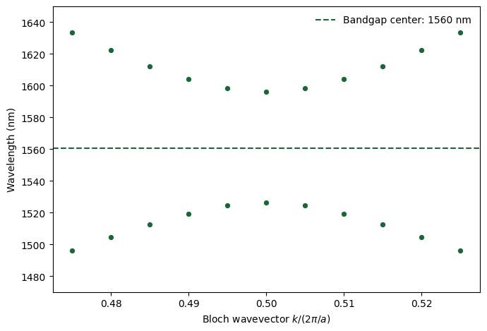
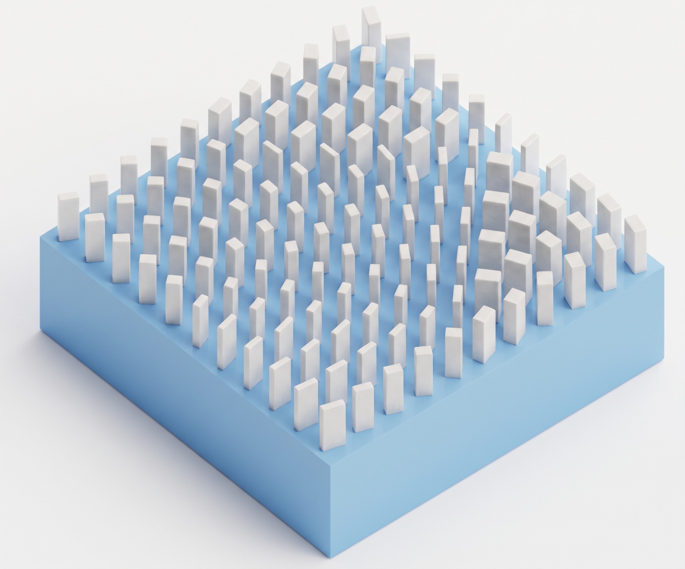
A one-dimensional periodic perturbation folds the guided-wave dispersion into the first Brillouin zone. Near the zone boundary, $k/(2\pi/a)=0.5$, counter-propagating Bloch waves become Bragg coupled. The periodic corrugation lifts their degeneracy and opens a photonic bandgap whose center and width depend on the average modal index and on the strength of the periodic perturbation. Here, the unit-cell parameters are chosen to place the bandgap center near 1.56 $\mathrm{\mu m}$.
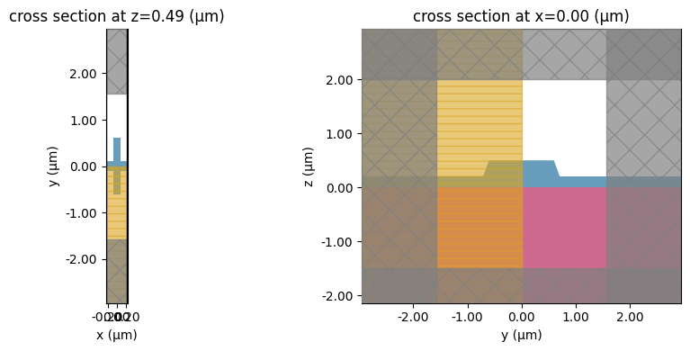
The unit cell consists of a narrow central backbone and symmetric corrugation teeth, with the tooth length set by the duty cycle. Randomly positioned $E_y$ dipoles excite the Bloch modes, while FieldTimeMonitors record the ring-down signals. Bloch boundary conditions are applied along the propagation direction, and the resonant frequencies are extracted using ResonanceFinder as the Bloch wavevector is swept around the Brillouin-zone edge.
def make_unit_cell_simulation(period, film_thickness, etch_depth, backbone_width, corrugation_width, bloch_k):
    slab_thickness = film_thickness - etch_depth
    tooth_length = period * duty_cycle
    y_inner = backbone_width / 2
    y_outer = y_inner + corrugation_width

    structures = [
        td.Structure(geometry=td.PolySlab(vertices=[(-100, y_inner), (100, y_inner), (100, -y_inner), (-100, -y_inner)],axis=2, slab_bounds=(slab_thickness, film_thickness),
            sidewall_angle=sidewall_angle, reference_plane="top"), medium=ln),
        td.Structure(geometry=td.Box(center=(0, 0, slab_thickness / 2), size=(td.inf, td.inf, slab_thickness)), medium=ln),
        td.Structure(geometry=td.Box(center=(0, 0, -50), size=(td.inf, td.inf, 100)), medium=silica)]

    for vertices in [
        [(-tooth_length / 2, y_inner), (tooth_length / 2, y_inner),
            (tooth_length / 2, y_outer), (-tooth_length / 2, y_outer)],
        [(-tooth_length / 2, -y_inner), (tooth_length / 2, -y_inner),
            (tooth_length / 2, -y_outer), (-tooth_length / 2, -y_outer)]
            ]:
        structures.append(
            td.Structure(
                geometry=td.PolySlab(vertices=vertices, axis=2, slab_bounds=(slab_thickness, film_thickness),
                sidewall_angle=sidewall_angle, reference_plane="top"), medium=ln))

    rng = np.random.default_rng(12345)

    dipole_positions = rng.uniform(
        [-1.2 * tooth_length / 2, 0, slab_thickness + etch_depth / 2],
        [1.2 * tooth_length / 2, y_outer, slab_thickness + etch_depth / 2],
        [10, 3])

    dipole_phases = rng.uniform(0, 2 * np.pi, 10)

    monitor_positions = rng.uniform(
        [-1.2 * tooth_length / 2, 0, slab_thickness + etch_depth / 2],
        [1.2 * tooth_length / 2, y_outer, slab_thickness + etch_depth / 2],
        [4, 3])

    sources = []
    for i in range(10):
        sources.append(
            td.PointDipole(
                center=tuple(dipole_positions[i]), polarization="Ey",
                source_time=td.GaussianPulse(freq0=freq0, fwidth=fwidth, phase=dipole_phases[i]),
                name=f"dipole_{i}",
            )
        )

    monitors = []
    for i in range(4):
        monitors.append(
            td.FieldTimeMonitor(
                center=tuple(monitor_positions[i]), size=(0, 0, 0), fields=["Ey"],
                start=t_start, name=f"monitor_time_{i}",
            )
        )

    return td.Simulation(
        center=(0, 0, film_thickness / 2),
        size=(period, backbone_width + 2 * corrugation_width + 1.5 + period, 2 * 1.5 + film_thickness),
        grid_spec=td.GridSpec.auto(min_steps_per_wvl=20),
        structures=structures, sources=sources, monitors=monitors,
        run_time=run_time, shutoff=0, normalize_index=None, symmetry=(0, -1, 0), medium=air,
        boundary_spec=td.BoundarySpec(
            x=td.Boundary.bloch(bloch_k), y=td.Boundary.absorber(), z=td.Boundary.pml()
        ),
    )
num_k = 11
k_values = np.linspace(0.475, 0.525, num_k)

band_simulations = {}
for i, bloch_k in enumerate(k_values):
    band_simulations[f"sim_{i}"] = make_unit_cell_simulation(
        period_um, film_thickness_um, etch_depth_um,
        backbone_width_um, corrugation_width_um, bloch_k,
    )

fig, axes = plt.subplots(1, 2, figsize=(10, 4), tight_layout=True)
band_simulations["sim_0"].plot(z=film_thickness_um - 0.01, ax=axes[0])
band_simulations["sim_0"].plot(x=0, freq=freq0, ax=axes[1])
plt.show()
Run the band-structure simulations
The simulations for different Bloch wavevectors are independent and are submitted together as a Batch.
band_batch = web.Batch(simulations=band_simulations, verbose=True)
band_results = band_batch.run()
Output()
02:42:23 EDT Started working on Batch containing 11 tasks.
02:42:35 EDT Maximum FlexCredit cost: 0.368 for the whole batch.
             Use 'Batch.real_cost()' to get the billed FlexCredit cost after
             completion.
Output()
02:43:29 EDT Batch complete.
Extract and plot the band structure
ResonanceFinder is used to extract the Bloch-mode frequencies from the time-domain monitor signals at each wavevector. Resonances with small amplitudes or large fitting errors are removed before plotting the band structure.
resonance_finder = ResonanceFinder(freq_window=(freq0 - fwidth, freq0 + fwidth))
zone_edge_freqs = None

fig, ax = plt.subplots(figsize=(7, 4.8), tight_layout=True)

for i, bloch_k in enumerate(k_values):
    resonance_data = resonance_finder.run(signals=band_results[f"sim_{i}"].data)
    resonance_data = resonance_data.where(abs(resonance_data.Q) > 0, drop=True)
    resonance_data = resonance_data.where(resonance_data.amplitude > 1, drop=True)
    resonance_data = resonance_data.where(resonance_data.error < 100, drop=True)

    frequencies = resonance_data.freq.to_numpy()
    wavelengths_nm = 1000 * td.C_0 / frequencies

    ax.scatter(np.full(len(wavelengths_nm), bloch_k), wavelengths_nm, s=18, color="C0")

    if np.isclose(bloch_k, 0.5):
        zone_edge_freqs = frequencies

band_edges = zone_edge_freqs[np.argsort(abs(zone_edge_freqs - freq0))[:2]]
bandgap_center_nm = 1000 * td.C_0 / np.mean(band_edges)

ax.axhline(bandgap_center_nm, linestyle="--", label=f"Bandgap center: {bandgap_center_nm:.0f} nm")

ax.set_xlabel(r"Bloch wavevector $k/(2\pi/a)$")
ax.set_ylabel("Wavelength (nm)")
ax.set_ylim(1470, 1650)
ax.legend(frameon=False)

plt.show()
Input waveguide design from the Bragg condition
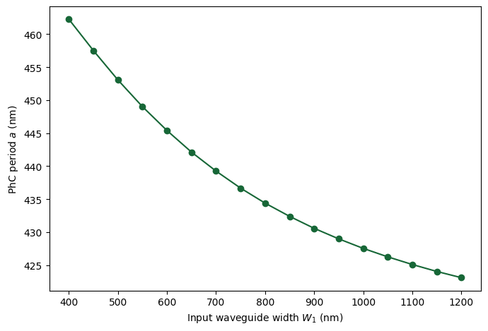
The PhC reflector is connected to an uncorrugated access waveguide through an apodized transition to reduce mode mismatch between the guided mode and the Bloch mode of the strongly corrugated PhC. The initial access-waveguide width $W_1$ is chosen using the first-order Bragg condition
$$ 2n_{\mathrm{eff}}a=\lambda_{\mathrm{B}}, $$
where $n_{\mathrm{eff}}$ is the effective index of the fundamental mode of the uncorrugated waveguide, $a$ is the PhC period, and $\lambda_{\mathrm{B}}$ is the target Bragg wavelength.
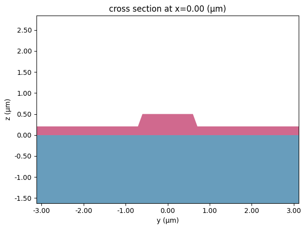
The calculation below sweeps $W_1$, evaluates $n_{\mathrm{eff}}$, and converts it to the corresponding Bragg period. The width matching the chosen period gives the input-waveguide design point. Note that $W_1$ is the width of the uncorrugated access waveguide and is distinct from the narrow PhC backbone width $W_2$. The full photonic bandgap is determined from the periodic unit-cell calculation above.
waveguide_widths_um = np.linspace(0.40, 1.20, 17)
mode_solvers = {}

for waveguide_width_um in waveguide_widths_um:
    task_name = f"width={waveguide_width_um:.3f}"
    cross_section = waveguide.RectangularDielectric(
        wavelength=target_wavelength_um, core_width=waveguide_width_um,
        core_thickness=film_thickness_um, slab_thickness=slab_thickness_um,
        sidewall_angle=sidewall_angle, core_medium=ln,
        clad_medium=air, box_medium=silica,
        mode_spec=td.ModeSpec(num_modes=1, num_pml=(12, 12), precision="double"))
    mode_solvers[task_name] = cross_section.mode_solver

cross_section.plot_structures(x=0)
plt.show()
mode_batch = web.Batch(simulations=mode_solvers, verbose=True)
mode_results = mode_batch.run()
Output()
02:44:02 EDT Started working on Batch containing 17 tasks.
02:44:17 EDT Maximum FlexCredit cost: 0.066 for the whole batch.
             Use 'Batch.real_cost()' to get the billed FlexCredit cost after
             completion.
Output()
02:44:50 EDT Batch complete.
widths_um = []
periods_um = []

for task_name, mode_data in mode_results.items():
    waveguide_width_um = float(task_name.split("=")[-1])
    effective_index = np.real(mode_data.n_eff.isel(mode_index=0, f=0).item())
    widths_um.append(waveguide_width_um)
    periods_um.append(target_wavelength_um / (2 * effective_index))

order = np.argsort(widths_um)
widths_um = np.asarray(widths_um)[order]
periods_um = np.asarray(periods_um)[order]

selected_width_um = np.interp(period_um, periods_um[::-1], widths_um[::-1])
print(f"Waveguide width for a = {1000 * period_um:.0f} nm: {1000 * selected_width_um:.1f} nm")

fig, ax = plt.subplots(figsize=(7, 4.8), tight_layout=True)
ax.plot(1000 * widths_um, 1000 * periods_um, "o-")

ax.set_xlabel(r"Input waveguide width $W_1$ (nm)")
ax.set_ylabel(r"PhC period $a$ (nm)")

plt.show()
Waveguide width for a = 445 nm: 606.1 nm
Apodized Bragg reflector
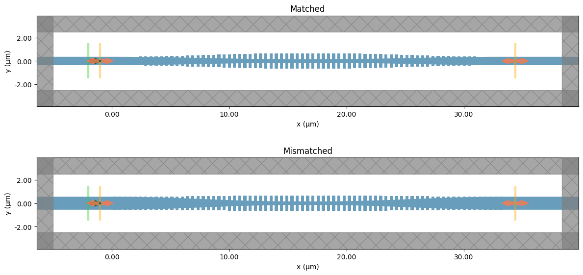
An abrupt transition from the access waveguide to the strongly corrugated PhC can cause mode mismatch between the propagating guided mode and the PhC Bloch mode. To reduce this mismatch, both the central backbone width and the corrugation width are varied smoothly through an apodized transition.
The finite reflector consists of a uniform PhC section between two symmetric apodized transitions. We compare the Bragg-matched input width obtained above with a deliberately mismatched wider waveguide and evaluate their reflection, transmission, and guided-mode leakage using 3D FDTD.
taper_cells = 35
main_cells = 5

def make_reflector_simulation(input_width, freqs):
    taper_length = taper_cells * period_um
    main_length = main_cells * period_um
    device_length = 2 * taper_length + main_length

    def apodization_ratio(x):
        if x < 0 or x > device_length:
            return 0
        if x <= taper_length:
            return (np.sin((x / taper_length - 0.5) * np.pi) + 1) / 2
        if x <= taper_length + main_length:
            return 1
        return (np.sin(((device_length - x) / taper_length - 0.5) * np.pi) + 1) / 2

    x_left = np.linspace(0, taper_length, 200)
    x_main = np.linspace(taper_length, taper_length + main_length, 50)
    x_right = np.linspace(taper_length + main_length, device_length, 200)
    x_backbone = np.concatenate(([-100, 0], x_left[1:], x_main[1:], x_right[1:], [device_length + 100]))

    y_backbone = np.array([
        (input_width + (backbone_width_um - input_width) * apodization_ratio(x)) / 2
        for x in x_backbone
    ])
    backbone_vertices = np.vstack((
        np.column_stack((x_backbone, y_backbone)),
        np.column_stack((x_backbone[::-1], -y_backbone[::-1])),
    ))

    structures = [
        td.Structure(
            geometry=td.PolySlab(
                vertices=backbone_vertices, axis=2,
                slab_bounds=(-etch_depth_um / 2, etch_depth_um / 2),
                sidewall_angle=sidewall_angle, reference_plane="top",
            ),
            medium=ln,
        )
    ]

    duty_start = 0.5 - duty_cycle / 2
    duty_end = 0.5 + duty_cycle / 2
    for i in range(2 * taper_cells + main_cells):
        tooth_start = (i + duty_start) * period_um
        tooth_end = (i + duty_end) * period_um
        tooth_center = (tooth_start + tooth_end) / 2
        ratio = apodization_ratio(tooth_center)

        local_backbone_width = input_width + (backbone_width_um - input_width) * ratio
        local_corrugation_width = corrugation_width_um * ratio
        y_inner = local_backbone_width / 2
        y_outer = y_inner + local_corrugation_width

        for vertices in [
            [(tooth_start, y_inner), (tooth_end, y_inner), (tooth_end, y_outer), (tooth_start, y_outer)],
            [(tooth_start, -y_inner), (tooth_end, -y_inner), (tooth_end, -y_outer), (tooth_start, -y_outer)],
        ]:
            structures.append(
                td.Structure(
                    geometry=td.PolySlab(
                        vertices=vertices, axis=2,
                        slab_bounds=(-etch_depth_um / 2, etch_depth_um / 2),
                        sidewall_angle=sidewall_angle, reference_plane="top",
                    ),
                    medium=ln,
                )
            )

    structures.extend([
        td.Structure(
            geometry=td.Box.from_bounds(
                rmin=(-100, -100, -etch_depth_um / 2 - slab_thickness_um),
                rmax=(100, 100, -etch_depth_um / 2),
            ),
            medium=ln,
        ),
        td.Structure(
            geometry=td.Box.from_bounds(
                rmin=(-100, -100, -100),
                rmax=(100, 100, -etch_depth_um / 2 - slab_thickness_um),
            ),
            medium=silica,
        ),
    ])

    mode_source = td.ModeSource(
        center=(-2, 0, 0), size=(0, 3, 3), mode_index=0, direction="+",
        source_time=td.GaussianPulse(
            freq0=(np.min(freqs) + np.max(freqs)) / 2,
            fwidth=(np.max(freqs) - np.min(freqs)) / 3,
        ),
        mode_spec=td.ModeSpec(num_modes=1), num_freqs=7,
    )

    monitors = [
        td.ModeMonitor(
            center=(-1, 0, 0), size=(0, 3, 3), freqs=freqs,
            mode_spec=td.ModeSpec(num_modes=1), name="mode_refl",
        ),
        td.ModeMonitor(
            center=(device_length + 1, 0, 0), size=(0, 3, 3), freqs=freqs,
            mode_spec=td.ModeSpec(num_modes=1), name="mode_trans",
        ),
    ]

    sim_x_min = -5
    sim_x_max = device_length + 5
    simulation = td.Simulation(
        center=((sim_x_min + sim_x_max) / 2, 0, 0),
        size=(sim_x_max - sim_x_min, 5, film_thickness_um + 3),
        grid_spec=td.GridSpec.auto(min_steps_per_wvl=20),
        structures=structures, sources=[mode_source], monitors=monitors,
        run_time=10e-12,
        boundary_spec=td.BoundarySpec(
            x=td.Boundary.absorber(), y=td.Boundary.absorber(), z=td.Boundary.absorber()
        ),
    )
    return simulation
The Bragg-matched input width obtained above is compared with a deliberately mismatched wider waveguide while keeping the PhC geometry unchanged.
reflector_freqs = np.linspace(freq0 - fwidth, freq0 + fwidth, 400)

reflector_simulations = {}
for label, input_width in {"matched": selected_width_um, "mismatched": 1.0}.items():
    reflector_simulations[label] = make_reflector_simulation(input_width, reflector_freqs)

fig, axes = plt.subplots(2, 1, figsize=(12, 6), tight_layout=True)
for ax, (label, simulation) in zip(axes, reflector_simulations.items()):
    simulation.plot(z=0, ax=ax)
    ax.set_title(label.capitalize())

plt.show()
reflector_batch = web.Batch(simulations=reflector_simulations, verbose=True)
reflector_results = reflector_batch.run()
Output()
02:45:00 EDT Started working on Batch containing 2 tasks.
02:45:07 EDT Maximum FlexCredit cost: 12.298 for the whole batch.
             Use 'Batch.real_cost()' to get the billed FlexCredit cost after
             completion.
Output()
02:46:29 EDT Batch complete.
Reflectance and guided-mode leakage
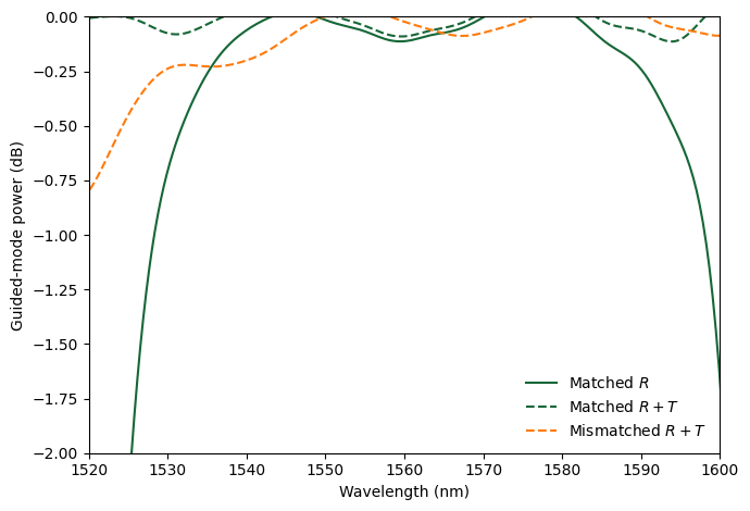
If the optical power remains in the monitored fundamental waveguide mode, $1-(R+T)$ stays close to unity. Since the material models are lossless, a reduction in $1-(R+T)$ primarily indicates coupling to radiation, slab, or higher-order modes.
The matched reflectance is plotted together with $1-(R+T)$ for both input-waveguide designs. This distinguishes reduced reflection caused by transmission from power coupled out of the monitored fundamental modes.
fig, ax = plt.subplots(figsize=(7, 4.8), tight_layout=True)

for label, color in zip(["matched", "mismatched"], ["C0", "C1"]):
    refl_amps = reflector_results[label]["mode_refl"].amps.sel(direction="-", mode_index=0)
    trans_amps = reflector_results[label]["mode_trans"].amps.sel(direction="+", mode_index=0)

    wavelengths_nm = 1000 * td.C_0 / np.asarray(trans_amps.f.values)
    reflectance = np.abs(np.asarray(refl_amps.values).squeeze()) ** 2
    transmittance = np.abs(np.asarray(trans_amps.values).squeeze()) ** 2
    order = np.argsort(wavelengths_nm)

    r_db = 10 * np.log10(np.clip(reflectance, 1e-8, None))
    rt_db = 10 * np.log10(np.clip(reflectance + transmittance, 1e-8, None))

    if label == "matched":
        ax.plot(wavelengths_nm[order], r_db[order], color=color, label="Matched $R$")

    ax.plot(wavelengths_nm[order], rt_db[order], "--", color=color, label=f"{label.capitalize()} $R+T$")

ax.set_xlabel("Wavelength (nm)")
ax.set_ylabel("Guided-mode power (dB)")
ax.set_xlim(1520, 1600)
ax.set_ylim(-2, 0)
ax.legend(frameon=False)

plt.show()
Short-wavelength loss
The mismatched input waveguide shows a larger reduction in $R+T$ toward the short-wavelength side of the reflection band, indicating increased coupling out of the monitored fundamental mode. A similar behavior was reported by Hwang et al., where the additional short-wavelength loss of a non-optimized transition was attributed to excitation of a leaky slab mode.
The $R+T$ spectrum identifies the presence of modal leakage but does not uniquely determine the destination of the missing power. Field profiles or additional modal analysis would be required to distinguish radiation, slab-mode excitation, and higher-order mode conversion.
Effect of LN film thickness
The present notebook considers a fixed LN film thickness, but the same workflow can be extended to study its influence on the reflector design. In general, a thinner LN film can produce a wider photonic bandgap, whereas a thicker film tends to provide stronger vertical confinement but a narrower bandgap and greater involvement of higher-order modes.
For each film thickness, the unit-cell band structure can be recalculated, followed by the Bragg-condition analysis to determine the corresponding input-waveguide width. The finite-reflector FDTD simulation can then be repeated to compare the reflection bandwidth and guided-mode leakage.


 TERMS & CONDITIONS


 How the process works:
 Try this real URL to see an example: