





Jay Zou, Tarik Cigeroglu Department of Applied Physics, Yale University, New Haven, CT 06511
Motivation. We want a smarter alternative to the standard uniform-radius minimum-feature-size filter used in topology optimization. Our hypothesis: a moderate uniform filter can be replaced by a spatially varying filter that allows smaller features in low-sensitivity regions of the design and keeps coarser features in high-sensitivity regions, so that fabrication and material errors do not affect the device performance in proportion to feature density. The adjoint method already produces $\partial J/\partial \rho$ for free at every Adam step, so we use that signal directly to modulate the filter radius — no CNN surrogate needed (cf. Park et al. arXiv 2510.22176, 2025, who used integrated-gradient attribution of a surrogate as a post-hoc explanation tool).
We demonstrate the intervention on a 2D wavelength-division demultiplexer following the Autograd9WDM tutorial: one run with the standard uniform filter and one with our adaptive filter, identical in every other respect (Adam, learning rate, $\beta$ schedule, penalty, init). We then compare the two converged designs against each other and under several fabrication-noise models.
Reproducibility. The notebook ships with all simulation results pre-cached; the rendered HTML reflects those cached results. Each cell that loads a cache is a cache-or-dispatch fallback — if a cache is missing or partial, the cell rebuilds the relevant simulations and submits them to the Tidy3D cloud cluster, then merges the results back into the cache. So a full re-run from scratch is supported (web.run_async will be called inside the notebook with chunked, retry-protected batches), but in practice the cached data is enough for the figures.
If you are unfamiliar with inverse design or topology optimization, the intro tutorials and the adjoint primer are good starting points.
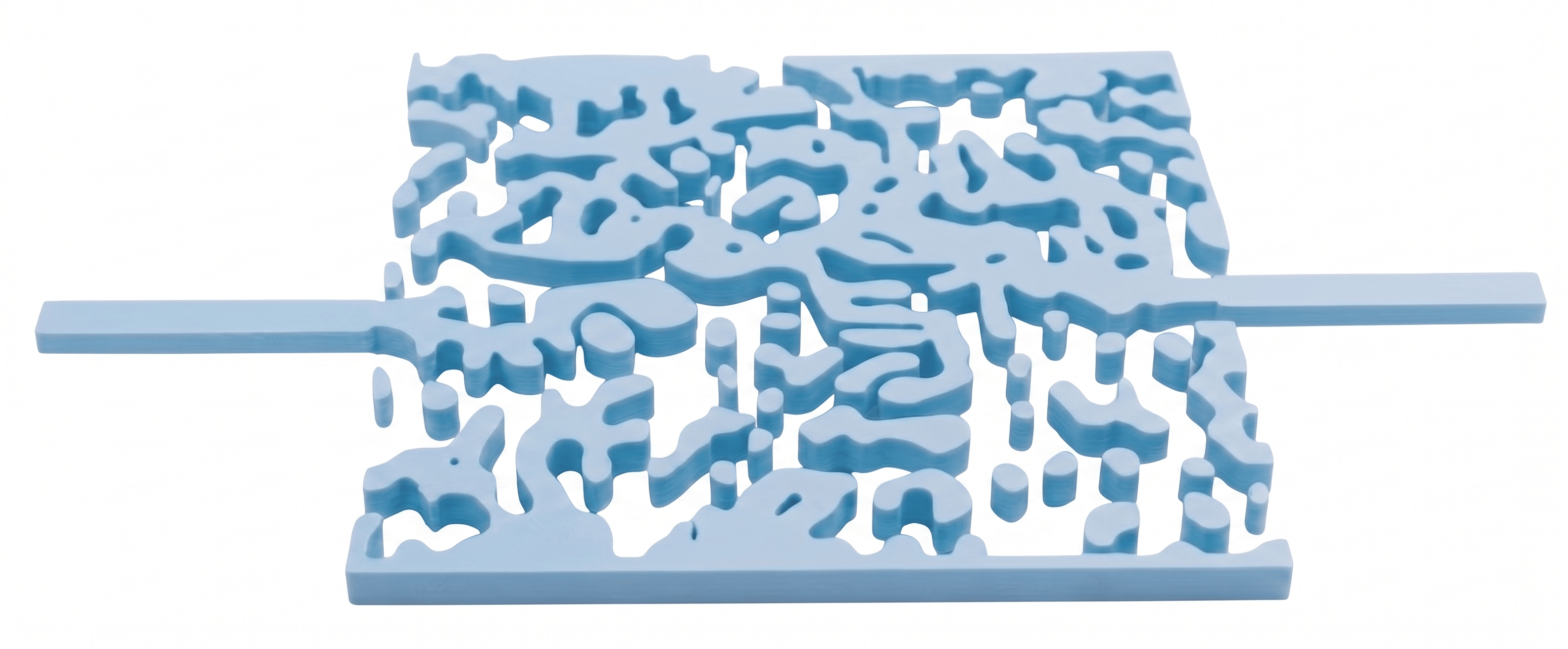
Revised conclusions — read before the results below
This notebook was originally written comparing the adaptive filter against a uniform $r = 100$ nm baseline. That comparison moves two variables at once, because the adaptive filter's floor is $r_{\rm low} = 50$ nm. We have since trained the matched-floor control — a plain uniform filter at 50 nm — and it overturns most of the original conclusions:
- 77% of the reported nominal gain is the finer feature size, not sensitivity-driven reallocation. Sum-FoM 3.399 → 3.711 → 3.807 for baseline → control → adaptive; only $+0.096$ of the $+0.408$ is attributable to the mechanism, from a single seed.
- The plain 50 nm control is more robust than the adaptive filter, winning 11 of 17 CD-jitter amplitudes and 16 of 17 microloading amplitudes on own-baseline retention. There is no simple "coarse features are robust" law either — on absolute FoM the 100 nm baseline is the worst device from ratio 0.1 to 5 and has the largest small-noise curvature. Its one decisive win, at ratio 10, resisted three attempted explanations and is reported as unexplained.
- The "routes around sensitivity hot spots" result is a boundary-length artifact — the control, which has no sensitivity information, reproduces it (11.3% vs 11.0%).
- The online variant performed far worse than any other device and we do not yet know why; hypotheses are in the Discussion.
What survives: the adaptive run has the most monotonic training trajectory (86% improving steps vs 71% control, 63% baseline), which feature size does not explain.
The reason the effect is so small is measurable: under $\max$ normalization the blend map leaves 99.9% of pixels within a fraction of a nm of $r_{\rm low}$, so what was actually tested is a uniform 50 nm filter. The idea is not refuted — it has not really been tested. See the Discussion for what would test it.
Sections below are presented in their original order; the analysis cells and the Discussion carry the corrected numbers.
Setup
Imports, channel parameters, geometric parameters. We use autograd.numpy as anp for any quantity that flows into the EM solver gradient — plain numpy for cached-data and statistics work.
import json
from pathlib import Path

import autograd as ag
import autograd.numpy as anp
import matplotlib.pyplot as plt
import numpy as np
import tidy3d as td
import tidy3d.web as web

from tidy3d.plugins.autograd import (
    adam, apply_updates,
    make_erosion_dilation_penalty,
    make_filter_and_project,
    rescale,
    smooth_min,
)

# All cached results ship with the notebook under the shared `misc/` data folder,
# so every figure below re-renders from disk without dispatching a simulation.
RESULTS_DIR = Path("misc/sens_aware_training"); RESULTS_DIR.mkdir(parents=True, exist_ok=True)
SIMDATA_DIR = RESULTS_DIR / "sim_data"; SIMDATA_DIR.mkdir(exist_ok=True)


from contextlib import contextmanager

@contextmanager
def quiet_tidy3d(level="ERROR"):
    '''Temporarily raise the tidy3d log level around a bulk dispatch.

    The accessor moved in Tidy3D 2.12 (`td.config.logging_level` ->
    `td.config.logging.level`) and the old name now raises AttributeError, so
    try the new location first and fall back for older versions.
    '''
    try:
        holder, attr = td.config.logging, "level"        # tidy3d >= 2.12
        prev = getattr(holder, attr)
    except AttributeError:
        holder, attr = td.config, "logging_level"        # tidy3d < 2.12
        prev = getattr(holder, attr)
    setattr(holder, attr, level)
    try:
        yield
    finally:
        setattr(holder, attr, prev)


print(f"tidy3d {td.__version__}")
tidy3d 2.12.0
Spend guard
Every cell that can dispatch to the cloud is gated by a hard FlexUnit ceiling. check_budget raises before anything is uploaded or started, so an over-budget cell costs nothing rather than discovering the problem halfway through a batch.
The per-simulation rates below are measured from this project's own completed-task history (web.get_tasks → realFlexUnit), not guessed. At the current cap, 3 FlexUnits buys roughly 40 perturbed sims or 68 average sims — enough for the small one-off evaluations, and deliberately not enough for a training run (~250 sims) or a Monte-Carlo sweep (~1020 sims). Those are all cached; if you genuinely intend to re-run one, raise MAX_FLEX_UNITS on purpose and re-execute.
# ---------------- hard spend ceiling ----------------
# What this notebook is permitted to dispatch. Every dispatch site carries a tag:
#   "training"    50-step optimization runs        ~6.7 FU each
#   "eval"        converged-device evaluation      ~0.03 FU
#   "spectrum"    151-freq spectrum                ~0.03 FU
#   "sensitivity" one forward+adjoint              ~0.17 FU
#   "mc"          Monte-Carlo sweep                ~74.6 FU
#   "ed"          erosion-dilation sweep           ~0.80 FU
#
#   False            -> nothing may dispatch (safe for re-rendering from cache)
#   True             -> anything may dispatch, subject to MAX_FLEX_UNITS
#   {"training", …}  -> only the listed tags; everything else skips or blocks
#
# Currently armed for the schedule-variant run: its training (~6.72 FU) plus the eval
# and spectrum sims (~0.07 FU) it needs to enter the geometry, spectral and sensitivity
# comparisons. Monte-Carlo and erosion-dilation dispatch are refused even though "ed"
# would fit under the cap.
ALLOW_DISPATCH = {"eval", "spectrum"}        # re-render from cache only: nothing may dispatch

MAX_FLEX_UNITS = 1.0        # ceiling on one dispatch AND on the session total.


def dispatch_allowed(tag):
    """Is a dispatch of this category permitted by ALLOW_DISPATCH?"""
    if ALLOW_DISPATCH is True:
        return True
    if not ALLOW_DISPATCH:
        return False
    return tag in ALLOW_DISPATCH

# Measured from this project's completed tasks (realFlexUnit / task), 2026-08.
FU_PER_SIM = {
    "perturbed": 0.0731,    # MC / ED forward sims (151-freq monitors)
    "forward":   0.0344,    # eval / spectrum / training forward
    "adjoint":   0.0250,    # adjoint solves
    "default":   0.0438,
}
# One Adam step = 1 forward + 1 adjoint per output monitor. Defined as a function
# because num_freqs_design is set in the next cell.
def fu_per_train_step(n_channels):
    return FU_PER_SIM["forward"] + n_channels * FU_PER_SIM["adjoint"]


class BudgetExceeded(RuntimeError):
    """Raised before any upload when a dispatch would exceed MAX_FLEX_UNITS."""


def estimate_fu(n_sims, kind="default"):
    return n_sims * FU_PER_SIM.get(kind, FU_PER_SIM["default"])


SESSION_FU_SPENT = 0.0      # running total of everything dispatched this session


def check_budget(n_sims, label, kind="default", fu=None, quiet=False,
                 tag="other", accrue=True):
    """Gate a dispatch. Raises BudgetExceeded *before* upload if not permitted.

    `tag` is checked against ALLOW_DISPATCH. MAX_FLEX_UNITS caps BOTH a single
    dispatch and the cumulative session total, so a long chain of individually-small
    dispatches cannot creep past it either.

    `accrue=False` validates permission without charging the session total — used by
    the per-step backstop inside the objective, whose cost is already reserved by the
    enclosing training-loop guard. Without it the loop would be counted twice.
    """
    global SESSION_FU_SPENT
    est = estimate_fu(n_sims, kind) if fu is None else fu
    remaining = MAX_FLEX_UNITS - SESSION_FU_SPENT
    if not dispatch_allowed(tag):
        raise BudgetExceeded(
            f"\n  BLOCKED: '{label}' (tag '{tag}') would submit {n_sims} simulation(s) "
            f"~= {est:.2f} FlexUnits.\n"
            f"  ALLOW_DISPATCH = {ALLOW_DISPATCH!r} does not permit '{tag}'.\n"
            f"  NOTHING was uploaded or started."
        )
    if not accrue:
        return est
    if est > MAX_FLEX_UNITS or est > remaining:
        raise BudgetExceeded(
            f"\n  BLOCKED: '{label}' would submit {n_sims} simulation(s) ~= {est:.2f} FlexUnits.\n"
            f"  Already dispatched this session: {SESSION_FU_SPENT:.2f} FU.  "
            f"Remaining under cap: {remaining:.2f} FU  (MAX_FLEX_UNITS = {MAX_FLEX_UNITS}).\n"
            f"  NOTHING was uploaded or started.\n"
            f"  This result is probably already cached in {RESULTS_DIR}/ — check the cache\n"
            f"  filename in this cell. To dispatch anyway, raise MAX_FLEX_UNITS deliberately."
        )
    SESSION_FU_SPENT += est
    if not quiet:
        print(f"  [budget] {label}: {n_sims} sim(s) ~= {est:.2f} FU   "
              f"(session {SESSION_FU_SPENT:.2f} / {MAX_FLEX_UNITS})")
    return est
# material indices
n_si  = 3.49
n_air = 1.0

# four channel wavelengths (O-band CWDM grid)
wvls_design     = np.array([1.270, 1.290, 1.310, 1.330])
freqs_design    = td.C_0 / wvls_design
num_freqs_design = len(freqs_design)
freq_max, freq_min = freqs_design.max(), freqs_design.min()
df_design          = abs(np.mean(np.diff(freqs_design)))
freq0   = float(np.mean(freqs_design))
fwidth  = float(freq_max - freq_min)
run_time = 200 / fwidth

# channel-averaging frequencies (each channel's metric is averaged over a small bandwidth)
channel_fwidth = df_design / 2.0
channel_bounds = [(f - channel_fwidth/2, f + channel_fwidth/2) for f in freqs_design]
num_freqs_channel = 5
channel_freqs = []
for fmin, fmax in channel_bounds:
    channel_freqs += np.linspace(fmin, fmax, num_freqs_channel).tolist()

# geometry — design region (square), waveguides, simulation extents
lx, ly      = 4.5, 4.5
ly_single   = ly / num_freqs_design
lz          = td.inf

wg_width, wg_length = 0.3, 1.5
buffer = 1.5
Lx, Ly, Lz = lx + 2*wg_length, ly + 2*buffer, 0.0   # 2D simulation

# fabrication knobs
radius           = 0.100
beta0            = 2
beta_penalty     = 10
min_steps_per_wvl = 18
dl_design_region  = 0.015
nx = int(lx / dl_design_region)
ny = int(ly / dl_design_region)

print(f"design region: {nx} x {ny} = {nx*ny:,} pixels at dl = {dl_design_region*1e3:.0f} nm")
print(f"channels     : {num_freqs_design} ({wvls_design.tolist()} um)")
design region: 300 x 300 = 90,000 pixels at dl = 15 nm
channels     : 4 ([1.27, 1.29, 1.31, 1.33] um)
Static simulation
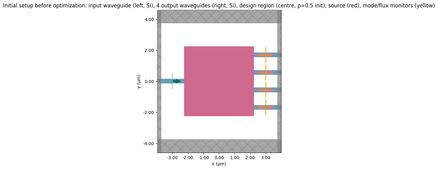
A single input waveguide on the left, four output waveguides on the right (one per channel), and a square design region in the middle. We add a ModeMonitor and a FluxMonitor per output, plus one field monitor at $z = 0$.
# input waveguide
wg_in = td.Structure(
    geometry=td.Box(center=(-Lx/2, 0, 0), size=(2*wg_length, wg_width, lz)),
    medium=td.Medium(permittivity=n_si**2),
)
# four output waveguides
centers_y = np.linspace(-ly/2 + ly_single/2, +ly/2 - ly_single/2, num_freqs_design)
mode_size = (0, 0.9 * ly_single, td.inf)
wgs_out = [
    td.Structure(
        geometry=td.Box(center=(+Lx/2, cy, 0), size=(2*wg_length, wg_width, lz)),
        medium=td.Medium(permittivity=n_si**2),
    )
    for cy in centers_y
]

# per-output mode monitor (transmission per mode)
mnts_mode = [
    td.ModeMonitor(
        center=(Lx/2 - wg_length/2, cy, 0), size=mode_size,
        freqs=channel_freqs, mode_spec=td.ModeSpec(),
        name=f"mode_{i}",
    )
    for i, cy in enumerate(centers_y)
]
# per-output flux monitor (kept for diagnostics)
mnts_flux = [
    td.FluxMonitor(
        center=(Lx/2 - wg_length/2, cy, 0), size=mode_size,
        freqs=channel_freqs, name=f"flux_{i}",
    )
    for i, cy in enumerate(centers_y)
]
# field monitor at the design plane
fld_mnt = td.FieldMonitor(
    center=(0, 0, 0), size=(td.inf, td.inf, 0),
    freqs=freqs_design, name="field",
)

# input source (fundamental mode)
mode_src = td.ModeSource(
    center=(-Lx/2 + wg_length/2, 0, 0), size=mode_size,
    source_time=td.GaussianPulse(freq0=freq0, fwidth=fwidth),
    direction="+", mode_index=0,
)

sim_static = td.Simulation(
    size=(Lx, Ly, Lz),
    grid_spec=td.GridSpec.auto(min_steps_per_wvl=min_steps_per_wvl, wavelength=float(np.min(wvls_design))),
    structures=[wg_in] + wgs_out,
    sources=[mode_src],
    monitors=mnts_mode + mnts_flux + [fld_mnt],
    boundary_spec=td.BoundarySpec.pml(x=True, y=True, z=False),
    run_time=run_time,
)

design_region_geo = td.Box(size=(lx, ly, lz), center=(0, 0, 0))

# Build an init sim with a uniform rho=0.5 design region so the design region
# is visible in the setup plot (sim_static alone has no structure inside it).
_eps_init = n_air**2 + (n_si**2 - n_air**2) * 0.5     # midpoint epsilon
_xs = np.linspace(-lx/2, lx/2, nx)
_ys = np.linspace(-ly/2, ly/2, ny)
_eps_init_field = _eps_init * np.ones((nx, ny, 1))
_init_design = td.Structure(
    geometry=design_region_geo,
    medium=td.CustomMedium(permittivity=td.ScalarFieldDataArray(
        data=_eps_init_field, coords=dict(x=_xs, y=_ys, z=[0]))),
)
_sim_init = sim_static.updated_copy(
    structures=list(sim_static.structures) + [_init_design],
)

fig, ax = plt.subplots(figsize=(11, 6))
_sim_init.plot(z=0.01, ax=ax)
ax.set_aspect('equal')
ax.set_title("Initial setup before optimization: input waveguide (left, Si), "
             "4 output waveguides (right, Si), design region (centre, ρ=0.5 init), "
             "source (red), mode/flux monitors (yellow)")
plt.show()
Design-region density, projection, and the (uniform) filter
The optimizer's design parameters are a continuous field $\rho \in [0, 1]^{n_x \times n_y}$. They flow through
$$\rho \;\xrightarrow{\text{filter}}\; \tilde\rho \;\xrightarrow{\text{tanh-}\beta\text{ project}}\; \bar\rho \;\xrightarrow{\text{interp}}\; \varepsilon \;\xrightarrow{\text{Maxwell}}\; J$$
The filter is a conic-kernel convolution that enforces a minimum feature size — features narrower than $\sim r/\sqrt{3}$ are blurred away. Without a filter, the optimizer happily produces single-pixel checkerboards that no foundry could fabricate.
make_filter_and_project from tidy3d.plugins.autograd returns the uniform-radius filter+project as a single autograd-traced function.
filter_uniform = make_filter_and_project(radius, dl_design_region)


def get_density(params, beta, filter_fn=filter_uniform):
    return filter_fn(params, beta=beta)


def make_eps(params, beta, filter_fn=filter_uniform):
    density = get_density(params, beta, filter_fn=filter_fn)
    return rescale(density, n_air**2, n_si**2)


def make_custom_medium_from_density(density):
    '''Design-region Structure built directly from the projected density rho_bar.'''
    eps = rescale(density, n_air**2, n_si**2).reshape((nx, ny, 1))
    xs = anp.linspace(-lx/2, lx/2, nx)
    ys = anp.linspace(-ly/2, ly/2, ny)
    coords = dict(x=xs, y=ys, z=[0])
    eps_arr = td.ScalarFieldDataArray(data=eps, coords=coords)
    return td.Structure(geometry=design_region_geo, medium=td.CustomMedium(permittivity=eps_arr))


def make_custom_medium(params, beta, filter_fn=filter_uniform):
    return make_custom_medium_from_density(get_density(params, beta, filter_fn=filter_fn))


def get_sim_from_density(density, include_extra_mnts=True):
    '''Simulation for a given projected density. The design-region mesh override is
    mandatory here - without it the auto-grid coarsens inside the design region and
    the FoM drops ~24% as a pure discretization artifact (see project notes).'''
    design = make_custom_medium_from_density(density)
    override = td.MeshOverrideStructure(
        geometry=design.geometry, dl=[dl_design_region]*3,
    )
    grid_spec = sim_static.grid_spec.updated_copy(
        override_structures=list(sim_static.grid_spec.override_structures) + [override]
    )
    update = dict(
        structures=list(sim_static.structures) + [design],
        grid_spec=grid_spec,
    )
    if not include_extra_mnts:
        update["monitors"] = mnts_mode
    return sim_static.updated_copy(**update)


def get_sim(params, beta, filter_fn=filter_uniform, include_extra_mnts=True):
    return get_sim_from_density(get_density(params, beta, filter_fn=filter_fn),
                                include_extra_mnts=include_extra_mnts)
Objective
Channel bands, not single frequencies. Each design frequency $f_i$ defines a band $[f_i - \Delta f / 2,\; f_i + \Delta f / 2]$ of width $\Delta f = (\text{inter-channel spacing})/2$, sampled by the mode monitors at 5 evenly-spaced sub-frequencies (channel_freqs in the setup cells). The per-channel transmitted power $T_{j,i}$ used in the metric below is the average of $|\text{amp}|^2$ across those 5 in-band samples (this is what average_over_channel and get_power compute). A device with a sharp transmission peak that drifts off the design wavelength gets no credit — the optimizer is being pushed to be flat across the channel, not perfect at one point. The colored bands in the spectral plots later in the notebook show these channel bandwidths.
For each channel $i$, the per-channel metric is
$$m_i = T_{i,i} - w \cdot \frac{1}{n-1}\sum_{j \ne i} T_{j,i}$$
where $T_{j,i}$ is the channel-averaged transmitted power at the band of frequency $j$ measured at output $i$, and $w$ (leak_weight) sets how aggressively we penalize cross-channel leakage. The total objective is smooth_min of these per-channel metrics, minus a feature-size penalty:
$$J_{\rm train} = \mathrm{smooth\_min}_i\bigl(m_i\bigr) \;-\; w_p \cdot \mathrm{penalty}(\rho)$$
The make_erosion_dilation_penalty from tidy3d.plugins.autograd rewards designs that are invariant under symmetric erosion and dilation by the filter radius — a soft minimum-feature-size constraint that complements the filter itself. Note that $J_{\rm train}$ contains the penalty term; we will distinguish it from the physical $J = \mathrm{smooth\_min}_i(m_i)$ (no penalty) used to evaluate actual device performance after training.
penalty = make_erosion_dilation_penalty(radius, dl_design_region, beta=beta_penalty)


def average_over_channel(spectrum, fmin, fmax):
    freqs = spectrum.f
    in_band = np.logical_and(freqs >= fmin, freqs <= fmax).values
    return spectrum.values @ in_band / np.sum(in_band)


def get_power(sim_data, mnt_index, freq_index):
    mnt_data = sim_data[mnts_mode[mnt_index].name]
    fmin_c, fmax_c = channel_bounds[freq_index]
    amp = mnt_data.amps.sel(direction="+", mode_index=0)
    spectrum = anp.abs(amp)**2
    return average_over_channel(spectrum, fmin=fmin_c, fmax=fmax_c)


def get_metric(sim_data, mnt_index, leak_weight=1.0):
    power_all = [get_power(sim_data, mnt_index=mnt_index, freq_index=j)
                 for j in range(num_freqs_design)]
    power_transmitted = power_all[mnt_index]
    power_leaked = sum(power_all) - power_transmitted
    return power_transmitted - leak_weight * power_leaked / (num_freqs_design - 1)


def make_objective(filter_fn):
    def objective(params, beta, penalty_weight=1.0, leak_weight=0.0):
        sim = get_sim(params, beta=beta, filter_fn=filter_fn, include_extra_mnts=False)
        check_budget(1, "objective solve", "forward", quiet=True, tag="training", accrue=False)
        sim_data = web.run(sim, task_name="autograd9wdm",
                           path=str(SIMDATA_DIR / "training.hdf5"),
                           verbose=False)
        all_metrics = [get_metric(sim_data, mnt_index=i, leak_weight=leak_weight)
                       for i in range(num_freqs_design)]
        metric = smooth_min(anp.array(all_metrics))
        penalty_value = penalty(params)
        return metric - penalty_weight * penalty_value
    return objective


def metric_of_density(density, leak_weight=0.0):
    '''The physical objective as a function of the projected density rho_bar (no filter,
    no penalty). Differentiating this gives dJ/d(rho_bar) - the sensitivity of performance
    to the *manufactured* structure, which is what fabrication error actually perturbs.'''
    sim = get_sim_from_density(density, include_extra_mnts=False)
    check_budget(1, "objective solve", "forward", quiet=True, tag="training", accrue=False)
    sim_data = web.run(sim, task_name="autograd9wdm",
                       path=str(SIMDATA_DIR / "training.hdf5"), verbose=False)
    all_metrics = [get_metric(sim_data, mnt_index=i, leak_weight=leak_weight)
                   for i in range(num_freqs_design)]
    return smooth_min(anp.array(all_metrics))


def value_and_grads(params, beta, filter_fn, penalty_weight=1.0, leak_weight=0.0):
    '''One forward + one adjoint solve, returning three things:

        J_train      = metric - penalty_weight * penalty          (float)
        dJ_train/dparams                                          (for Adam)
        dmetric/d(rho_bar)                                        (for the filter map)

    The parameter gradient is obtained by chaining dmetric/d(rho_bar) back through the
    filter's VJP, so it is *identical* to ag.value_and_grad(make_objective(f)) - Adam is
    unaffected. The extra output costs nothing: dJ/d(rho_bar) is already an intermediate
    of the same backward pass. The filter VJP and the penalty are pure NumPy.
    '''
    vjp_filter, rho_bar = ag.make_vjp(lambda x: filter_fn(x, beta=beta))(params)
    metric_val, g_density = ag.value_and_grad(
        lambda d: metric_of_density(d, leak_weight=leak_weight))(rho_bar)
    g_params_metric = vjp_filter(g_density)

    pen_val, g_pen = ag.value_and_grad(penalty)(params)
    J_train = float(metric_val) - penalty_weight * float(pen_val)
    g_train = np.asarray(g_params_metric) - penalty_weight * np.asarray(g_pen)
    return J_train, g_train, np.asarray(g_density)
Optimization with the standard uniform filter
We run 50 Adam iterations with lr = 0.1, $\beta$ annealed from 1 to 50, and leak_weight ramped from 0 to 1 after the first third of training. The starting parameters are the deterministic uniform field $\rho = 0.5 \cdot \mathbf{1}$ (the choice in Autograd9WDM).
The cell below uses a cache: if results/wdm_uniform_optim.json already exists, it is loaded directly; otherwise we run the full optimization. Re-running this notebook after the first run is then a cache hit (a few seconds) instead of a fresh training.
num_steps     = 50
learning_rate = 0.1
beta_min, beta_max = 1, 50

CACHE_UNIFORM = RESULTS_DIR / "wdm_uniform_optim.json"


def train(filter_fn, label):
    # One Adam step = 1 forward + num_freqs_design adjoint solves.
    check_budget(num_steps * (1 + num_freqs_design), f"training[{label}]",
                 fu=num_steps * fu_per_train_step(num_freqs_design), tag="training")
    obj_fn = make_objective(filter_fn)
    grad_fn = ag.value_and_grad(obj_fn)
    np.random.seed(0)
    params0 = np.random.random((nx, ny))
    params  = 0.5 * np.ones_like(params0)
    optimizer = adam(learning_rate=learning_rate)
    opt_state = optimizer.init(params)
    Js, beta_history, penalty_history = [], [], []
    for i in range(num_steps):
        perc = i / (num_steps - 1)
        beta_i = beta_min * (1 - perc) + beta_max * perc
        leak_weight = 0.0 if perc < 1/3 else 1.0
        value, gradient = grad_fn(params, beta=beta_i,
                                  penalty_weight=1.0, leak_weight=leak_weight)
        pen = float(penalty(params))
        J_phys = float(value) + pen   # physical J = smooth_min(channels), no penalty
        print(f"  [{label}] step {i+1:>2}: J_phys = {J_phys:+.4f}  "
              f"(J_train = {float(value):+.4f}, penalty = {pen:.4f}, beta = {beta_i:.1f})",
              flush=True)
        updates, opt_state = optimizer.update(-gradient, opt_state, params)
        params[:] = apply_updates(params, updates)
        np.clip(params, 0.0, 1.0, out=params)
        Js.append(float(value))
        beta_history.append(float(beta_i))
        penalty_history.append(pen)
    return params, Js, beta_history, penalty_history


if CACHE_UNIFORM.exists():
    print(f"cache hit: {CACHE_UNIFORM}")
    u = json.loads(CACHE_UNIFORM.read_text())
else:
    print(f"cache miss: running uniform-filter optimization")
    obj_fn = make_objective(filter_uniform)
    grad_fn = ag.value_and_grad(obj_fn)
    params, Js, beta_history, penalty_history = train(filter_uniform, "uniform")
    # save final-iteration sensitivity field for the sensitivity-aware run downstream
    _, final_grad = grad_fn(params, beta=beta_history[-1],
                            penalty_weight=1.0, leak_weight=1.0)
    u = dict(
        params_final     = params.tolist(),
        Js               = Js,
        beta_history     = beta_history,
        penalty_history  = penalty_history,
        sensitivity_field= np.asarray(final_grad).tolist(),
        nx=int(nx), ny=int(ny),
        radius=float(radius), dl_design_region=float(dl_design_region),
    )
    CACHE_UNIFORM.write_text(json.dumps(u))
    print(f"saved {CACHE_UNIFORM}")

params_uniform   = np.array(u['params_final'])
sensitivity_field = np.abs(np.array(u['sensitivity_field']))
beta_final = u['beta_history'][-1]
rho_uniform = np.array(filter_uniform(params_uniform, beta=beta_final))

print()
print(f"converged after {len(u['Js'])} iterations at beta = {beta_final:.0f}")
print(f"final training J = {u['Js'][-1]:+.4f}  (= smooth_min(channels) - penalty)")
print(f"binarization     : {(rho_uniform < 0.05).mean()*100:.1f}% void / "
      f"{(rho_uniform > 0.95).mean()*100:.1f}% solid / "
      f"{((rho_uniform > 0.05) & (rho_uniform < 0.95)).mean()*100:.1f}% gray")
cache hit: misc/sens_aware_training/wdm_uniform_optim.json

converged after 50 iterations at beta = 50
final training J = -0.7218  (= smooth_min(channels) - penalty)
binarization     : 51.6% void / 45.9% solid / 2.6% gray
Loss-history and converged design
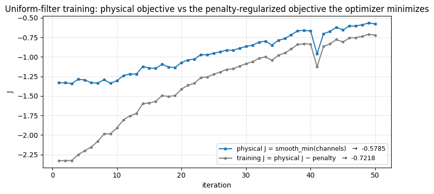
The training-J trajectory shows the optimizer climbing out of the gray-scale initial state into a binarized configuration. Recall this $J_{\rm train}$ contains the penalty term — the physical $J = \mathrm{smooth\_min}(\text{channels})$ at the converged design (no penalty) is computed in the next cell and shown as a horizontal annotation.
# Evaluate the converged uniform device (1 simulation). The full SimulationData is cached
# as an HDF5 at misc/sens_aware_training/sim_data/uniform_eval.hdf5; summary metrics in the
# JSON below.
CACHE_UNIFORM_EVAL = RESULTS_DIR / "wdm_uniform_eval.json"
SIM_UNIFORM_EVAL  = SIMDATA_DIR  / "uniform_eval.hdf5"

if CACHE_UNIFORM_EVAL.exists() and SIM_UNIFORM_EVAL.exists():
    eval_u = json.loads(CACHE_UNIFORM_EVAL.read_text())
    sd_uniform = td.SimulationData.from_file(str(SIM_UNIFORM_EVAL))
else:
    check_budget(1, "uniform eval", "forward", tag="eval")
    print("evaluating converged uniform device (1 simulation)")
    sim_eval = get_sim(params_uniform, beta=beta_final,
                       filter_fn=filter_uniform, include_extra_mnts=True)
    sd_uniform = web.run(sim_eval, task_name="wdm_uniform_eval",
                         path=str(SIM_UNIFORM_EVAL), verbose=False)
    transmissions = []  # 4 ports x N channel freqs
    for i in range(num_freqs_design):
        amps = sd_uniform[mnts_mode[i].name].amps.sel(direction="+", mode_index=0)
        transmissions.append((np.abs(np.asarray(amps))**2).flatten().tolist())
    channel_metrics_u = [float(get_metric(sd_uniform, mnt_index=i, leak_weight=1.0))
                         for i in range(num_freqs_design)]
    physical_J_u = float(smooth_min(anp.array(channel_metrics_u)))
    eval_u = dict(
        channel_metrics = channel_metrics_u,
        physical_J = physical_J_u,
        transmissions = transmissions,
        channel_freqs = list(channel_freqs),
    )
    CACHE_UNIFORM_EVAL.write_text(json.dumps(eval_u))
    print(f"saved {CACHE_UNIFORM_EVAL}")

physical_J_u = eval_u['physical_J']
channel_metrics_u = np.array(eval_u['channel_metrics'])
transmissions_u   = np.array(eval_u['transmissions'])

print(f"converged uniform device:")
print(f"  per-channel m_i: {channel_metrics_u}")
print(f"  physical J = smooth_min(m_i) = {physical_J_u:+.4f}    (training J was {u['Js'][-1]:+.4f})")
converged uniform device:
  per-channel m_i: [0.91181283 0.85009451 0.82303724 0.74162708]
  physical J = smooth_min(m_i) = -0.5565    (training J was -0.7218)
# Loss-history plot: training J (with penalty) and physical J (smooth_min only) per iteration.
its = np.arange(1, len(u['Js'])+1)
J_phys_history_u = np.array(u['Js']) + np.array(u['penalty_history'])  # penalty_weight = 1

fig, ax = plt.subplots(figsize=(8, 4))
ax.plot(its, J_phys_history_u, marker='s', ms=3, color='tab:blue',
        label=f"physical J = smooth_min(channels)   →  {J_phys_history_u[-1]:+.4f}")
ax.plot(its, u['Js'],          marker='o', ms=3, color='tab:gray',
        label=f"training J = physical J − penalty   →  {u['Js'][-1]:+.4f}")
ax.set_xlabel('iteration')
ax.set_ylabel('J')
ax.set_title("Uniform-filter training: physical objective vs the penalty-regularized objective the optimizer minimizes")
ax.legend(loc='lower right', fontsize=9)
ax.grid(alpha=0.3)
plt.tight_layout()
plt.show()
Field profiles at the four design wavelengths
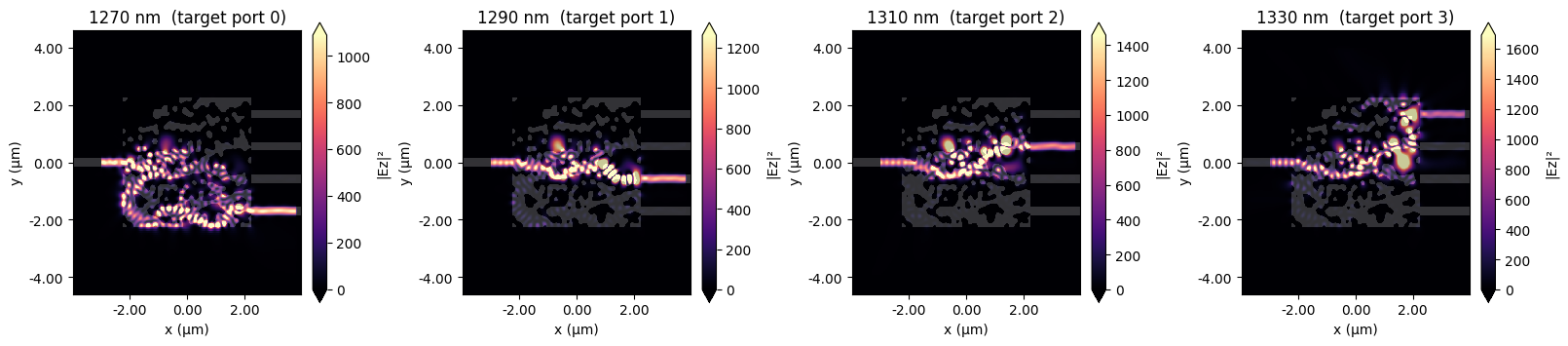
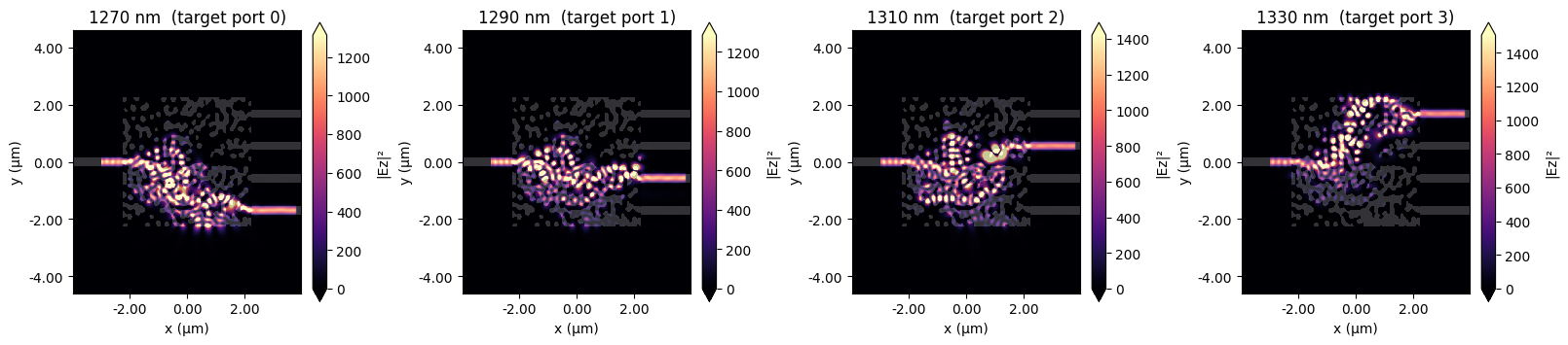
To see the device actually doing demultiplexing, we plot the out-of-plane component $|E_z|^2$ at each design wavelength on the $z = 0$ plane. (For our 2D ModeSource, the fundamental waveguide mode is TE-like with $E_z$ dominant.) Light enters from the input waveguide on the left and should preferentially exit through the corresponding output waveguide.
fig, axes = plt.subplots(1, num_freqs_design, figsize=(16, 3.5), constrained_layout=True)
for i, (freq, wvl) in enumerate(zip(freqs_design, wvls_design)):
    sd_uniform.plot_field('field', field_name='Ez', val='abs^2', f=float(freq), ax=axes[i])
    axes[i].set_title(f"{wvl*1e3:.0f} nm  (target port {i})")
plt.show()
Spectral response across the four channels
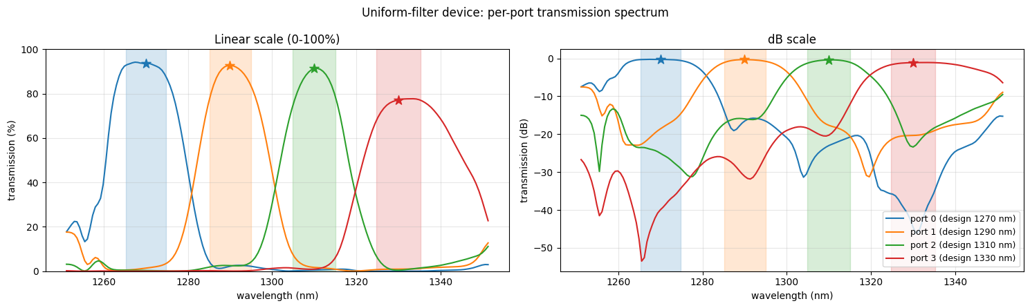
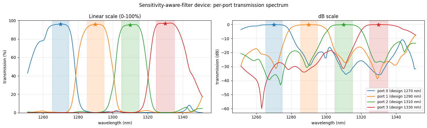
To confirm the converged uniform device is actually doing demultiplexing, we re-evaluate the device on a finer frequency grid (151 points across a wider range than the channel bands) and plot the per-port transmission in dB. A working demux shows each port's transmission peaking near 0 dB at its design wavelength and dropping sharply elsewhere. The shaded vertical bands mark each channel's bandwidth used by the optimizer; star markers sit at each design wavelength.
# Cache fine-grid spectrum (1 extra simulation per device).
CACHE_UNIFORM_SPECTRUM = RESULTS_DIR / "wdm_uniform_spectrum.json"
SIM_UNIFORM_SPECTRUM   = SIMDATA_DIR  / "uniform_spectrum.hdf5"

num_freqs_measure = 151
freqs_measure     = np.linspace(freq_min - df_design, freq_max + df_design, num_freqs_measure)

if CACHE_UNIFORM_SPECTRUM.exists():
    spec_u = json.loads(CACHE_UNIFORM_SPECTRUM.read_text())
else:
    check_budget(1, "uniform spectrum", "forward", tag="spectrum")
    print("computing fine-grid spectrum for uniform device (1 simulation, 151 freqs)")
    sim_spec = get_sim(params_uniform, beta=beta_final, filter_fn=filter_uniform, include_extra_mnts=True)
    for i in range(num_freqs_design):
        sim_spec = sim_spec.updated_copy(freqs=list(freqs_measure), path=f"monitors/{i}")
        sim_spec = sim_spec.updated_copy(freqs=list(freqs_measure), path=f"monitors/{i + num_freqs_design}")
    sd_spec = web.run(sim_spec, task_name="wdm_uniform_spectrum",
                      path=str(SIM_UNIFORM_SPECTRUM), verbose=False)
    powers_per_port = []
    for i in range(num_freqs_design):
        amps = sd_spec[mnts_mode[i].name].amps.sel(direction="+", mode_index=0)
        powers_per_port.append((np.abs(np.asarray(amps))**2).flatten().tolist())
    spec_u = dict(freqs_measure=list(freqs_measure), powers=powers_per_port)
    CACHE_UNIFORM_SPECTRUM.write_text(json.dumps(spec_u))
    print(f"saved {CACHE_UNIFORM_SPECTRUM}")

# Per-port transmission spectrum: linear (left, 0-100%) and dB (right). Tutorial style with
# shaded channel bands, star markers at each design wavelength, all 4 channels on each axes.
freqs_arr = np.array(spec_u['freqs_measure'])
wvls_nm   = 1000 * td.C_0 / freqs_arr
colors    = ['tab:blue', 'tab:orange', 'tab:green', 'tab:red']

fig, axes = plt.subplots(1, 2, figsize=(15, 4.5))
for i in range(num_freqs_design):
    powers = np.array(spec_u['powers'][i])
    loss_db = 10 * np.log10(np.maximum(powers, 1e-6))
    fmin, fmax = channel_bounds[i]
    label = f"port {i} (design {wvls_design[i]*1e3:.0f} nm)"
    idx_design = int(np.argmin(np.abs(freqs_arr - float(freqs_design[i]))))   # closest freq sample to design wvl

    axes[0].axvspan(1000 * td.C_0 / fmin, 1000 * td.C_0 / fmax, alpha=0.18, color=colors[i])
    axes[0].plot(wvls_nm, powers * 100, color=colors[i], label=label)
    axes[0].scatter([wvls_design[i]*1e3], [powers[idx_design] * 100], 100, marker='*', color=colors[i], zorder=5)

    axes[1].axvspan(1000 * td.C_0 / fmin, 1000 * td.C_0 / fmax, alpha=0.18, color=colors[i])
    axes[1].plot(wvls_nm, loss_db, color=colors[i], label=label)
    axes[1].scatter([wvls_design[i]*1e3], [loss_db[idx_design]], 100, marker='*', color=colors[i], zorder=5)

axes[0].set_xlabel("wavelength (nm)"); axes[0].set_ylabel("transmission (%)")
axes[0].set_title("Linear scale (0-100%)")
axes[0].set_ylim(0, 100)
axes[0].grid(True, alpha=0.3)

axes[1].set_xlabel("wavelength (nm)"); axes[1].set_ylabel("transmission (dB)")
axes[1].set_title("dB scale")
axes[1].grid(True, alpha=0.3)
axes[1].legend(fontsize=9, loc='lower right')

fig.suptitle("Uniform-filter device: per-port transmission spectrum")
plt.tight_layout()
plt.show()
Converged design with sensitivity overlay
We overlay the adjoint sensitivity $|\partial J / \partial \rho|$ on the converged design. Bright spots in the magma overlay identify regions whose perturbation costs the most performance — typically concentrated at high-curvature edges and topology bottlenecks of the converged geometry.
# Sensitivity heatmap as the background (full opacity); device edges as a thin white contour on top.
fig, ax = plt.subplots(figsize=(7, 7))
sens_img = ax.imshow(np.flipud(sensitivity_field.T), cmap='magma')
ax.contour(np.flipud(rho_uniform.T), levels=[0.5], colors='white', linewidths=0.5)
ax.set_title(r"$|\partial J / \partial \rho|$ at the converged uniform design"
             + f"\nrange = {abs(sensitivity_field.max()-sensitivity_field.min()):.2e},  "
             + f"mean = {sensitivity_field.mean():.2e}")
ax.axis('off')
plt.colorbar(sens_img, ax=ax, fraction=0.046, pad=0.02, label=r'$|\partial J / \partial \rho|$')
plt.tight_layout()
plt.show()
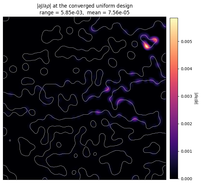
The sensitivity field is strongly heterogeneous. A handful of bright spots dominate; most of the design region has near-zero sensitivity, so the range of $|\partial J/\partial\rho|$ across the design region is much larger than its mean.
Park et al. made this observation rigorous on a similar device. They trained a CNN surrogate to predict transmission from binary masks, applied integrated gradients to attribute predicted performance to pixels, and then experimentally perturbed high- vs low-attribution pixels — the high-attribution perturbations caused up to 11× more excess insertion loss. They used this as a post-hoc explanation tool. The next section feeds the same signal back into the optimizer.
The sensitivity-driven adaptive filter
We make the filter radius spatially varying — larger in high-sensitivity regions (where small features would be fragile under fabrication noise) and smaller in low-sensitivity regions (where finer features carry no robustness penalty):
$$r(x, y) \;=\; r_{\rm low} + \alpha\,\bigl(r_{\rm high} - r_{\rm low}\bigr)\,\hat s(x, y), \qquad \hat s = |\partial J/\partial \rho|/\max|\partial J/\partial \rho| \in [0, 1]$$
A truly position-dependent conic kernel would require a custom convolution. Instead we use a much simpler two-radius blend: filter the design at $r_{\rm low}$ and $r_{\rm high}$ in parallel and combine them per pixel:
$$\bar\rho_{\rm adaptive}(x,y) \;=\; \bigl(1 - \alpha\,\hat s(x,y)\bigr)\,f_{r_{\rm low}}(\rho)(x,y) \;+\; \alpha\,\hat s(x,y)\,f_{r_{\rm high}}(\rho)(x,y)$$
Two convolutions per call instead of one; both are autograd-traced; the blend is differentiable.
def make_adaptive_filter_and_project(radius_low, radius_high, dl, sensitivity_field, alpha=1.0):
    f_low  = make_filter_and_project(radius_low,  dl)
    f_high = make_filter_and_project(radius_high, dl)

    s = anp.abs(anp.asarray(sensitivity_field, dtype=float))
    s_max = s.max()
    s_norm = s / s_max if s_max > 0 else s
    blend = alpha * s_norm

    def adaptive(params, beta):
        rho_low  = f_low(params,  beta=beta)
        rho_high = f_high(params, beta=beta)
        return (1.0 - blend) * rho_low + blend * rho_high

    return adaptive
The function returns a callable (params, beta) -> projected_density that matches the signature of make_filter_and_project. So substituting it into the pipeline above is one line — replace filter_uniform with the adaptive filter when constructing objective. We use the uniform-converged sensitivity field as a fixed input — i.e., one bootstrap uniform run gives us the filter for the sensitivity-aware run. An online-update variant (recompute every $K$ iterations) is a clean follow-up.
Optimization with the adaptive filter
We rerun the exact same training pipeline — same Adam, learning rate, $\beta$-anneal, penalty term, starting parameters — with only the filter swapped. The adaptive filter uses $r_{\rm low} = 50$ nm, $r_{\rm high} = 150$ nm, $\alpha = 1.0$, and the sensitivity field saved from the uniform run.
filter_sensaware = make_adaptive_filter_and_project(
    radius_low=0.05, radius_high=0.15, dl=dl_design_region,
    sensitivity_field=sensitivity_field, alpha=1.0,
)

CACHE_SENSAWARE = RESULTS_DIR / "wdm_sensaware_optim.json"

if CACHE_SENSAWARE.exists():
    print(f"cache hit: {CACHE_SENSAWARE}")
    s = json.loads(CACHE_SENSAWARE.read_text())
else:
    print(f"cache miss: running sensitivity-aware-filter optimization")
    params, Js, beta_history, penalty_history = train(filter_sensaware, "sensitivity-aware")
    s = dict(
        params_final = params.tolist(),
        Js           = Js,
        beta_history = beta_history,
        penalty_history = penalty_history,
        nx=int(nx), ny=int(ny),
        radius_low=0.05, radius_high=0.15, alpha=1.0,
        dl_design_region=float(dl_design_region),
    )
    CACHE_SENSAWARE.write_text(json.dumps(s))
    print(f"saved {CACHE_SENSAWARE}")

params_sensaware = np.array(s['params_final'])
rho_sensaware = np.array(filter_sensaware(params_sensaware, beta=s['beta_history'][-1]))

print()
print(f"converged after {len(s['Js'])} iterations at beta = {s['beta_history'][-1]:.0f}")
cache hit: misc/sens_aware_training/wdm_sensaware_optim.json

converged after 50 iterations at beta = 50
Loss-history and converged design (sensitivity-aware)
We compute the same physical-J at the converged sensitivity-aware design, then plot both training trajectories on the same axes for direct comparison.
# Evaluate sensitivity-aware device — physical J + transmissions + SimulationData (for fields).
CACHE_SENSAWARE_EVAL = RESULTS_DIR / "wdm_sensaware_eval.json"
SIM_SENSAWARE_EVAL  = SIMDATA_DIR  / "sensaware_eval.hdf5"

if CACHE_SENSAWARE_EVAL.exists() and SIM_SENSAWARE_EVAL.exists():
    eval_s = json.loads(CACHE_SENSAWARE_EVAL.read_text())
    sd_sensaware = td.SimulationData.from_file(str(SIM_SENSAWARE_EVAL))
else:
    check_budget(1, "sens-aware eval", "forward", tag="eval")
    print("evaluating converged sensitivity-aware device (1 simulation)")
    sim_eval = get_sim(params_sensaware, beta=s['beta_history'][-1],
                       filter_fn=filter_sensaware, include_extra_mnts=True)
    sd_sensaware = web.run(sim_eval, task_name="wdm_sensaware_eval",
                           path=str(SIM_SENSAWARE_EVAL), verbose=False)
    transmissions = []
    for i in range(num_freqs_design):
        amps = sd_sensaware[mnts_mode[i].name].amps.sel(direction="+", mode_index=0)
        transmissions.append((np.abs(np.asarray(amps))**2).flatten().tolist())
    channel_metrics_s = [float(get_metric(sd_sensaware, mnt_index=i, leak_weight=1.0))
                         for i in range(num_freqs_design)]
    physical_J_s = float(smooth_min(anp.array(channel_metrics_s)))
    eval_s = dict(
        channel_metrics = channel_metrics_s,
        physical_J = physical_J_s,
        transmissions = transmissions,
        channel_freqs = list(channel_freqs),
    )
    CACHE_SENSAWARE_EVAL.write_text(json.dumps(eval_s))
    print(f"saved {CACHE_SENSAWARE_EVAL}")

physical_J_s = eval_s['physical_J']
channel_metrics_s = np.array(eval_s['channel_metrics'])
transmissions_s   = np.array(eval_s['transmissions'])

print(f"converged sensitivity-aware device:")
print(f"  per-channel m_i: {channel_metrics_s}")
print(f"  physical J = smooth_min(m_i) = {physical_J_s:+.4f}    (training J was {s['Js'][-1]:+.4f})")
converged sensitivity-aware device:
  per-channel m_i: [0.94653369 0.93805664 0.93346438 0.95773431]
  physical J = smooth_min(m_i) = -0.4424    (training J was -0.6799)
# Combined loss-history: physical J (left) and training J (right), both devices overlaid.
its = np.arange(1, len(u['Js'])+1)
J_phys_u = np.array(u['Js']) + np.array(u['penalty_history'])
J_phys_s = np.array(s['Js']) + np.array(s['penalty_history'])

fig, axes = plt.subplots(1, 2, figsize=(13, 4), sharey=True)

axes[0].plot(its, J_phys_u, marker='s', ms=3, color='tab:blue',   label=f"uniform           → {J_phys_u[-1]:+.3f}")
axes[0].plot(its, J_phys_s, marker='s', ms=3, color='tab:purple', label=f"sensitivity-aware → {J_phys_s[-1]:+.3f}")
axes[0].set_xlabel('iteration')
axes[0].set_ylabel('J')
axes[0].set_title("Physical J  =  smooth_min(channels), no penalty")
axes[0].legend(loc='lower right', fontsize=9)
axes[0].grid(alpha=0.3)

axes[1].plot(its, u['Js'], marker='o', ms=3, color='tab:blue',   label=f"uniform           → {u['Js'][-1]:+.3f}")
axes[1].plot(its, s['Js'], marker='o', ms=3, color='tab:purple', label=f"sensitivity-aware → {s['Js'][-1]:+.3f}")
axes[1].set_xlabel('iteration')
axes[1].set_title("Training J  =  physical J  −  penalty   (what the optimizer minimizes)")
axes[1].legend(loc='lower right', fontsize=9)
axes[1].grid(alpha=0.3)

plt.tight_layout()
plt.show()
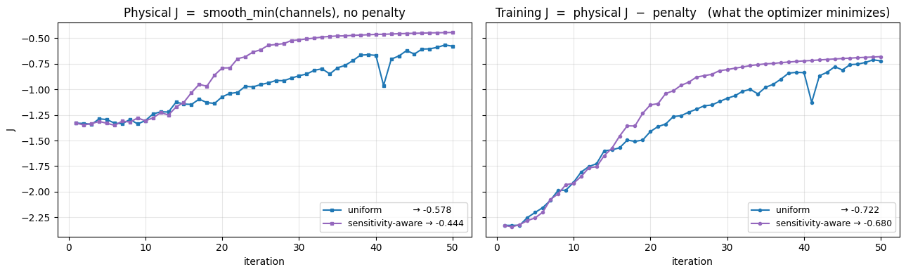
Reading these curves. Left panel: physical $J = \mathrm{smooth\_min}(\text{channels})$ at each iteration — what we actually care about for device performance, no penalty. Right panel: training $J = $ physical $J - $ penalty, the regularized objective the optimizer minimizes. The vertical gap between corresponding curves across the two panels is the converged penalty value (sizable because make_erosion_dilation_penalty is a soft constraint). For actual device performance, look at the left panel, not the right. The MC below evaluates designs on the same physical metric (no penalty).
Analysis. The first thing we notice in the FoM evolution is that the sensitivity-aware run outperforms uniform throughout training, and reaches a higher converged physical-$J$. The trajectory is also notably more monotonic — the uniform curve has visible noisy plateaus and dips, whereas the sens-aware curve climbs steadily. We attribute the smoother climb to the adaptive filter: by relaxing the minimum feature size in low-sensitivity regions (where small features cost no robustness), the optimizer has more room to make small but useful local refinements at each Adam step instead of being clipped by a hard global feature-size floor. The same effect explains the higher converged value — the optimizer simply has access to a larger feasible-design space.
Field profiles for the sensitivity-aware device
Same $|E_z|^2$ plot at each design wavelength, this time on the sensitivity-aware converged design. Shared color scale across the four panels for direct cross-channel comparison.
fig, axes = plt.subplots(1, num_freqs_design, figsize=(16, 3.5), constrained_layout=True)
for i, (freq, wvl) in enumerate(zip(freqs_design, wvls_design)):
    sd_sensaware.plot_field('field', field_name='Ez', val='abs^2', f=float(freq), ax=axes[i])
    axes[i].set_title(f"{wvl*1e3:.0f} nm  (target port {i})")
plt.show()
Spectral response of the sensitivity-aware device
Same fine-grid spectral evaluation as we did for the uniform device, this time on the converged sensitivity-aware design.
CACHE_SENSAWARE_SPECTRUM = RESULTS_DIR / "wdm_sensaware_spectrum.json"
SIM_SENSAWARE_SPECTRUM   = SIMDATA_DIR  / "sensaware_spectrum.hdf5"

if CACHE_SENSAWARE_SPECTRUM.exists():
    spec_s = json.loads(CACHE_SENSAWARE_SPECTRUM.read_text())
else:
    check_budget(1, "sens-aware spectrum", "forward", tag="spectrum")
    print("computing fine-grid spectrum for sensitivity-aware device (1 simulation, 151 freqs)")
    sim_spec = get_sim(params_sensaware, beta=s['beta_history'][-1],
                       filter_fn=filter_sensaware, include_extra_mnts=True)
    for i in range(num_freqs_design):
        sim_spec = sim_spec.updated_copy(freqs=list(freqs_measure), path=f"monitors/{i}")
        sim_spec = sim_spec.updated_copy(freqs=list(freqs_measure), path=f"monitors/{i + num_freqs_design}")
    sd_spec = web.run(sim_spec, task_name="wdm_sensaware_spectrum",
                      path=str(SIM_SENSAWARE_SPECTRUM), verbose=False)
    powers_per_port = []
    for i in range(num_freqs_design):
        amps = sd_spec[mnts_mode[i].name].amps.sel(direction="+", mode_index=0)
        powers_per_port.append((np.abs(np.asarray(amps))**2).flatten().tolist())
    spec_s = dict(freqs_measure=list(freqs_measure), powers=powers_per_port)
    CACHE_SENSAWARE_SPECTRUM.write_text(json.dumps(spec_s))
    print(f"saved {CACHE_SENSAWARE_SPECTRUM}")

fig, axes = plt.subplots(1, 2, figsize=(15, 4.5))
for i in range(num_freqs_design):
    powers = np.array(spec_s['powers'][i])
    loss_db = 10 * np.log10(np.maximum(powers, 1e-6))
    fmin, fmax = channel_bounds[i]
    label = f"port {i} (design {wvls_design[i]*1e3:.0f} nm)"
    idx_design = int(np.argmin(np.abs(freqs_arr - float(freqs_design[i]))))

    axes[0].axvspan(1000 * td.C_0 / fmin, 1000 * td.C_0 / fmax, alpha=0.18, color=colors[i])
    axes[0].plot(wvls_nm, powers * 100, color=colors[i], label=label)
    axes[0].scatter([wvls_design[i]*1e3], [powers[idx_design] * 100], 100, marker='*', color=colors[i], zorder=5)

    axes[1].axvspan(1000 * td.C_0 / fmin, 1000 * td.C_0 / fmax, alpha=0.18, color=colors[i])
    axes[1].plot(wvls_nm, loss_db, color=colors[i], label=label)
    axes[1].scatter([wvls_design[i]*1e3], [loss_db[idx_design]], 100, marker='*', color=colors[i], zorder=5)

axes[0].set_xlabel("wavelength (nm)"); axes[0].set_ylabel("transmission (%)")
axes[0].set_title("Linear scale (0-100%)")
axes[0].set_ylim(0, 100)
axes[0].grid(True, alpha=0.3)

axes[1].set_xlabel("wavelength (nm)"); axes[1].set_ylabel("transmission (dB)")
axes[1].set_title("dB scale")
axes[1].grid(True, alpha=0.3)
axes[1].legend(fontsize=9, loc='lower right')

fig.suptitle("Sensitivity-aware-filter device: per-port transmission spectrum")
plt.tight_layout()
plt.show()
Geometry helpers
Feature-size measurement and the Simulation objects used for the geometry plots. All cross-device figures now live in a single "Comparison of all four devices" section further down, after the $r = 50$ nm control and the online filter have both been trained — comparing here would only show two of the four.
from scipy import ndimage

def _smallest_feature_nm(rho, dl_um):
    bw = rho > 0.5
    labels, _ = ndimage.label(bw)
    sizes = np.bincount(labels.ravel())[1:]
    return float(np.sqrt(sizes.min()) * dl_um * 1e3), int(len(sizes))

side_u, n_u = _smallest_feature_nm(rho_uniform, dl_design_region)
side_s, n_s = _smallest_feature_nm(rho_sensaware, dl_design_region)

params_init         = 0.5 * np.ones((nx, ny))
sim_init            = get_sim(params_init,      beta=beta0,                 filter_fn=filter_uniform,   include_extra_mnts=False)
sim_uniform_final   = get_sim(params_uniform,   beta=beta_final,            filter_fn=filter_uniform,   include_extra_mnts=False)
sim_sensaware_final = get_sim(params_sensaware, beta=s['beta_history'][-1], filter_fn=filter_sensaware, include_extra_mnts=False)

# Fine-grid wavelength axis shared by every spectral comparison downstream.
freqs_cmp = np.array(spec_u['freqs_measure'])
wvls_cmp  = 1000 * td.C_0 / freqs_cmp

print(f"uniform r=100nm : {n_u} solid features, smallest ~{side_u:.0f} nm")
print(f"sens-aware      : {n_s} solid features, smallest ~{side_s:.0f} nm")
print(f"~{((rho_uniform > 0.5) != (rho_sensaware > 0.5)).mean()*100:.0f}% of pixels flipped "
      f"solid<->void between these two converged designs.")
uniform r=100nm : 29 solid features, smallest ~113 nm
sens-aware      : 50 solid features, smallest ~103 nm
~34% of pixels flipped solid<->void between these two converged designs.
Sens-aware sensitivity field
One cloud forward+adjoint sim (cached) gives the converged sens-aware design's own sensitivity field. It is needed by the cross-device sensitivity figures in the comparison section below.
# === Sens-aware sensitivity field (cache-or-dispatch) ===
SENS_AWARE_SENS_CACHE = RESULTS_DIR / "sens_aware_sensitivity.json"
if SENS_AWARE_SENS_CACHE.exists():
    _sens_aware_data = json.loads(SENS_AWARE_SENS_CACHE.read_text())
    print(f"loaded {SENS_AWARE_SENS_CACHE}")
else:
    check_budget(1 + num_freqs_design, "sens-aware sensitivity", "forward", tag="sensitivity")
    print("sens-aware sensitivity cache missing — computing one forward+adjoint sim")
    obj_fn_s = make_objective(filter_sensaware)
    grad_fn_s = ag.value_and_grad(obj_fn_s)
    _val_s, _grad_s = grad_fn_s(params_sensaware,
                                 beta=s['beta_history'][-1],
                                 penalty_weight=1.0, leak_weight=1.0)
    _sens_aware_data = dict(
        sensitivity_field=np.asarray(_grad_s).tolist(),
        nx=int(nx), ny=int(ny),
        radius_low=0.05, radius_high=0.15, alpha=1.0,
        dl_design_region=float(dl_design_region),
    )
    SENS_AWARE_SENS_CACHE.write_text(json.dumps(_sens_aware_data))
    print(f"computed sens-aware physical J = {float(_val_s):+.4f}; saved {SENS_AWARE_SENS_CACHE}")

sensitivity_field_sensaware = np.abs(np.array(_sens_aware_data['sensitivity_field']))

def _sens_stats(field):
    return abs(field.max() - field.min()), field.mean()

_rng_u, _mean_u = _sens_stats(sensitivity_field)
_rng_s, _mean_s = _sens_stats(sensitivity_field_sensaware)

print(f"sensitivity   uniform:    range = {_rng_u:.3e}    mean = {_mean_u:.3e}")
print(f"sensitivity   sens-aware: range = {_rng_s:.3e}    mean = {_mean_s:.3e}")
loaded misc/sens_aware_training/sens_aware_sensitivity.json
sensitivity   uniform:    range = 5.848e-03    mean = 7.558e-05
sensitivity   sens-aware: range = 3.890e-03    mean = 2.074e-05
Control: uniform filter at the adaptive filter's floor ($r = 50$ nm)
Everything above compares a $r = 100$ nm uniform filter against an adaptive filter spanning $r \in [50, 150]$ nm. Those two differ in two ways at once: the adaptive filter modulates by sensitivity, and its floor is half the baseline's radius. Any win could be explained by the second alone — smaller minimum feature size means more design freedom, which is a well-known way to get a better nominal FoM and has nothing to do with sensitivity.
So we add the control that separates them: a uniform filter at $r = 50$ nm, matching the adaptive filter's floor.
$$\underbrace{r = 100\ \text{nm}}_{\text{original baseline}} \qquad \underbrace{r = 50\ \text{nm}}_{\textbf{this control}} \qquad \underbrace{r \in [50, 150]\ \text{nm}}_{\text{adaptive}}$$
Read against this control, the adaptive filter's question becomes the sharp one: given the same 50 nm floor, does coarsening the high-sensitivity regions to 150 nm buy anything? If the adaptive device beats uniform-50, spatial reallocation is doing real work. If it merely ties, the entire effect was the finer floor.
Everything else is held fixed, including the penalty. make_erosion_dilation_penalty stays at radius = 0.100 for this run, exactly as it is for the uniform-100 and adaptive runs — it is a soft constraint on the design, not part of the filter under test. Changing it here would reintroduce a second difference and defeat the purpose of the control.
filter_uniform50 = make_filter_and_project(0.05, dl_design_region)

CACHE_UNIFORM50 = RESULTS_DIR / "wdm_uniform50_optim.json"

if CACHE_UNIFORM50.exists():
    print(f"cache hit: {CACHE_UNIFORM50}")
    u50 = json.loads(CACHE_UNIFORM50.read_text())
else:
    print("cache miss: running uniform r=50nm control optimization (50 forward+adjoint sims)")
    _grad_fn_u50 = ag.value_and_grad(make_objective(filter_uniform50))
    _p50, _Js50, _beta50, _pen50 = train(filter_uniform50, "uniform-50nm")
    # final-iteration sensitivity, for the own-sensitivity comparison (no extra sim beyond this one)
    _val50, _g50 = _grad_fn_u50(_p50, beta=_beta50[-1], penalty_weight=1.0, leak_weight=1.0)
    u50 = dict(
        params_final      = _p50.tolist(),
        Js                = _Js50,
        beta_history      = _beta50,
        penalty_history   = _pen50,
        sensitivity_field = np.asarray(_g50).tolist(),
        nx=int(nx), ny=int(ny),
        radius=0.05, dl_design_region=float(dl_design_region),
    )
    CACHE_UNIFORM50.write_text(json.dumps(u50))
    print(f"saved {CACHE_UNIFORM50}")

params_uniform50 = np.array(u50['params_final'])
beta_final_u50   = u50['beta_history'][-1]
rho_uniform50    = np.array(filter_uniform50(params_uniform50, beta=beta_final_u50))
sensitivity_field_uniform50 = np.abs(np.array(u50['sensitivity_field']))

print()
print(f"converged after {len(u50['Js'])} iterations at beta = {beta_final_u50:.0f}")
print(f"final training J = {u50['Js'][-1]:+.4f}")
print(f"binarization     : {(rho_uniform50 < 0.05).mean()*100:.1f}% void / "
      f"{(rho_uniform50 > 0.95).mean()*100:.1f}% solid / "
      f"{((rho_uniform50 > 0.05) & (rho_uniform50 < 0.95)).mean()*100:.1f}% gray")
cache hit: misc/sens_aware_training/wdm_uniform50_optim.json

converged after 50 iterations at beta = 50
final training J = -0.6934
binarization     : 54.6% void / 43.7% solid / 1.7% gray
# Evaluate the converged uniform-50nm control (1 simulation).
CACHE_UNIFORM50_EVAL = RESULTS_DIR / "wdm_uniform50_eval.json"
SIM_UNIFORM50_EVAL   = SIMDATA_DIR  / "uniform50_eval.hdf5"

if CACHE_UNIFORM50_EVAL.exists() and SIM_UNIFORM50_EVAL.exists():
    eval_u50 = json.loads(CACHE_UNIFORM50_EVAL.read_text())
    sd_uniform50 = td.SimulationData.from_file(str(SIM_UNIFORM50_EVAL))
else:
    check_budget(1, "uniform50 eval", "forward", tag="eval")
    print("evaluating converged uniform-50nm device (1 simulation)")
    sim_eval = get_sim(params_uniform50, beta=beta_final_u50,
                       filter_fn=filter_uniform50, include_extra_mnts=True)
    sd_uniform50 = web.run(sim_eval, task_name="wdm_uniform50_eval",
                           path=str(SIM_UNIFORM50_EVAL), verbose=False)
    transmissions = []
    for i in range(num_freqs_design):
        amps = sd_uniform50[mnts_mode[i].name].amps.sel(direction="+", mode_index=0)
        transmissions.append((np.abs(np.asarray(amps))**2).flatten().tolist())
    channel_metrics_u50 = [float(get_metric(sd_uniform50, mnt_index=i, leak_weight=1.0))
                           for i in range(num_freqs_design)]
    eval_u50 = dict(
        channel_metrics = channel_metrics_u50,
        physical_J = float(smooth_min(anp.array(channel_metrics_u50))),
        transmissions = transmissions,
        channel_freqs = list(channel_freqs),
    )
    CACHE_UNIFORM50_EVAL.write_text(json.dumps(eval_u50))
    print(f"saved {CACHE_UNIFORM50_EVAL}")

physical_J_u50      = eval_u50['physical_J']
channel_metrics_u50 = np.array(eval_u50['channel_metrics'])

print("converged uniform-50nm control:")
print(f"  per-channel m_i: {channel_metrics_u50}")
print(f"  physical J = smooth_min(m_i) = {physical_J_u50:+.4f}    (training J was {u50['Js'][-1]:+.4f})")
print()
print("  --- the control comparison ---")
print(f"  uniform r=100nm   : {physical_J_u:+.4f}")
print(f"  uniform r= 50nm   : {physical_J_u50:+.4f}   (vs r=100nm: {physical_J_u50-physical_J_u:+.4f})")
print(f"  adaptive [50,150] : {physical_J_s:+.4f}   (vs r= 50nm: {physical_J_s-physical_J_u50:+.4f})")
converged uniform-50nm control:
  per-channel m_i: [0.95121521 0.92618063 0.89955647 0.89814326]
  physical J = smooth_min(m_i) = -0.4678    (training J was -0.6934)

  --- the control comparison ---
  uniform r=100nm   : -0.5565
  uniform r= 50nm   : -0.4678   (vs r=100nm: +0.0888)
  adaptive [50,150] : -0.4424   (vs r= 50nm: +0.0254)
# Fine-grid spectrum for the uniform-50nm control (1 simulation, 151 freqs).
CACHE_UNIFORM50_SPECTRUM = RESULTS_DIR / "wdm_uniform50_spectrum.json"
SIM_UNIFORM50_SPECTRUM   = SIMDATA_DIR  / "uniform50_spectrum.hdf5"

if CACHE_UNIFORM50_SPECTRUM.exists():
    spec_u50 = json.loads(CACHE_UNIFORM50_SPECTRUM.read_text())
else:
    check_budget(1, "uniform50 spectrum", "forward", tag="spectrum")
    print("computing fine-grid spectrum for uniform-50nm control (1 simulation, 151 freqs)")
    sim_spec = get_sim(params_uniform50, beta=beta_final_u50,
                       filter_fn=filter_uniform50, include_extra_mnts=True)
    for i in range(num_freqs_design):
        sim_spec = sim_spec.updated_copy(freqs=list(freqs_measure), path=f"monitors/{i}")
        sim_spec = sim_spec.updated_copy(freqs=list(freqs_measure), path=f"monitors/{i + num_freqs_design}")
    sd_spec = web.run(sim_spec, task_name="wdm_uniform50_spectrum",
                      path=str(SIM_UNIFORM50_SPECTRUM), verbose=False)
    powers_per_port = []
    for i in range(num_freqs_design):
        amps = sd_spec[mnts_mode[i].name].amps.sel(direction="+", mode_index=0)
        powers_per_port.append((np.abs(np.asarray(amps))**2).flatten().tolist())
    spec_u50 = dict(freqs_measure=list(freqs_measure), powers=powers_per_port)
    CACHE_UNIFORM50_SPECTRUM.write_text(json.dumps(spec_u50))
    print(f"saved {CACHE_UNIFORM50_SPECTRUM}")

_side_u50, _n_u50 = _smallest_feature_nm(rho_uniform50, dl_design_region)
print(f"uniform-50nm control: {_n_u50} solid features, smallest ~{_side_u50:.0f} nm")
uniform-50nm control: 56 solid features, smallest ~95 nm
Online (per-iteration) sensitivity-aware filter
The adaptive filter used above is static: it is built once from the uniform-converged sensitivity field and then held fixed for all 50 Adam steps. But by iteration 40 the design no longer resembles the uniform design that produced that field, so the filter is modulating on an increasingly stale map.
The fix costs nothing. ag.value_and_grad already returns $\partial J/\partial\rho$ at every step — the same quantity we bootstrapped from. So we can rebuild the blend map from the current gradient after each step:
$$\hat s^{(k)} = \frac{|\partial J/\partial\rho\,|_{\rho^{(k)}}}{\mathcal{N}^{(k)}}, \qquad \bar\rho^{(k+1)} = \bigl(1 - \alpha\hat s^{(k)}\bigr) f_{r_{\rm low}}(\rho) + \alpha\hat s^{(k)} f_{r_{\rm high}}(\rho)$$
Zero extra simulations. The filter refresh reuses the gradient the optimizer already computed, so the online run costs exactly the same 50 forward+adjoint sims as the static run.
The blend map is frozen within a step. set_sensitivity stores a plain NumPy array, so autograd sees a constant during the backward pass of step $k$; the map only changes between steps. We are deliberately not differentiating through the filter-map update — that would be a second-order term ($\partial^2 J/\partial\rho^2$) which the adjoint method does not give us.
First: how much does the blend map actually modulate?
Before spending simulations, one diagnostic on the cached uniform sensitivity field — it decides how we normalize.
The static filter normalizes by $\max|\partial J/\partial\rho|$. That field is extremely heavy-tailed (as the plot above showed: a handful of bright spots, near-zero everywhere else), so dividing by the max squashes almost every pixel to $\hat s \approx 0$. The cell below quantifies what that means for the effective radius $r_{\rm eff} = r_{\rm low} + \hat s\,(r_{\rm high} - r_{\rm low})$ that each pixel actually sees.
# Pure post-processing on the cached uniform sensitivity field — no simulations.
def blend_from_sensitivity(field, mode="max", percentile=99.0, alpha=1.0):
    """Normalize |dJ/drho| into a blend map in [0, 1]."""
    sf = np.abs(np.asarray(field, dtype=float))
    if mode == "max":
        denom = sf.max()
    elif mode == "percentile":
        denom = np.percentile(sf, percentile)
    else:
        raise ValueError(f"unknown normalization mode: {mode!r}")
    if denom <= 0:
        return np.zeros_like(sf)
    return np.clip(alpha * sf / denom, 0.0, 1.0)


R_LOW_NM, R_HIGH_NM = 50.0, 150.0

_modes = [("max", None), ("percentile", 99.0), ("percentile", 95.0)]
print(f"Effective radius r_eff = {R_LOW_NM:.0f} + s_hat x ({R_HIGH_NM:.0f} - {R_LOW_NM:.0f}) nm, "
      f"over the {nx}x{ny} design region:\n")
print(f"{'normalization':<18}{'mean blend':>12}{'% px > 0.5':>12}{'mean r_eff':>13}{'median r_eff':>14}")
print("-" * 69)
_blend_demo = {}
for _mode, _pct in _modes:
    _b = blend_from_sensitivity(sensitivity_field, mode=_mode, percentile=_pct or 99.0)
    _label = _mode if _pct is None else f"{_mode} (p{_pct:g})"
    _blend_demo[_label] = _b
    _reff = R_LOW_NM + _b * (R_HIGH_NM - R_LOW_NM)
    print(f"{_label:<18}{_b.mean():>12.3f}{(_b > 0.5).mean()*100:>11.2f}%"
          f"{_reff.mean():>11.1f} nm{np.median(_reff):>12.1f} nm")

fig, axes = plt.subplots(1, len(_blend_demo) + 1, figsize=(4.1 * (len(_blend_demo) + 1), 4.0))
for ax, (_label, _b) in zip(axes, _blend_demo.items()):
    _reff = R_LOW_NM + _b * (R_HIGH_NM - R_LOW_NM)
    im = ax.imshow(np.flipud(_reff.T), cmap="viridis", vmin=R_LOW_NM, vmax=R_HIGH_NM)
    ax.contour(np.flipud(rho_uniform.T), levels=[0.5], colors="white", linewidths=0.4)
    ax.set_title(f"{_label}\nmean $r_{{eff}}$ = {_reff.mean():.1f} nm", fontsize=10)
    ax.axis("off")
    plt.colorbar(im, ax=ax, fraction=0.046, pad=0.02, label="$r_{eff}$ (nm)")

axes[-1].hist([_b.ravel() for _b in _blend_demo.values()], bins=40,
              label=list(_blend_demo.keys()), log=True)
axes[-1].set_xlabel(r"blend $\alpha\,\hat s$"); axes[-1].set_ylabel("pixel count (log)")
axes[-1].set_title("Blend distribution"); axes[-1].legend(fontsize=8); axes[-1].grid(alpha=0.3)
fig.suptitle("Effective filter radius under different sensitivity normalizations", fontsize=12)
plt.tight_layout()
plt.show()
Effective radius r_eff = 50 + s_hat x (150 - 50) nm, over the 300x300 design region:

normalization       mean blend  % px > 0.5   mean r_eff  median r_eff
---------------------------------------------------------------------
max                      0.013       0.12%       51.3 nm        50.3 nm
percentile (p99)         0.071       2.89%       57.1 nm        52.0 nm
percentile (p95)         0.176      10.68%       67.6 nm        56.4 nm
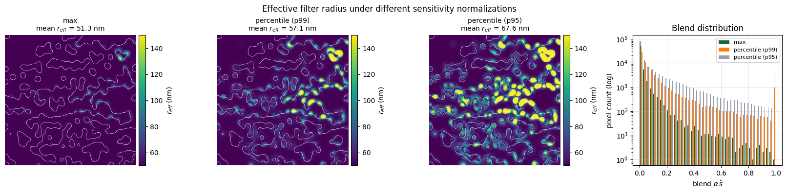
This is a significant caveat on the static result above. Under max normalization the median effective radius is ~50 nm — i.e. the static "adaptive" filter is, for the overwhelming majority of pixels, just a uniform 50 nm filter. Only a fraction of a percent of pixels are meaningfully pushed toward $r_{\rm high}$. So the static sens-aware win reported earlier is largely attributable to raw extra design freedom (50 nm vs the baseline's 100 nm) rather than to spatial reallocation — which is the caveat already flagged in the Discussion, now quantified.
It also matters for the online experiment specifically: refreshing a map that is $\approx 0$ almost everywhere would change almost nothing, and the online-vs-static comparison would return a null result for a purely numerical reason. Normalizing by a high percentile instead (with clipping at 1) keeps the map scale-free but actually exercises the two-radius mechanism. ONLINE_NORM below selects the mode, and the cache filenames are tagged with it, so both variants can be run and kept side by side.
The online filter
Same two-radius blend, but the map lives in a mutable closure that the training loop refreshes.
def make_online_adaptive_filter(radius_low, radius_high, dl,
                                alpha=1.0, mode="percentile", percentile=99.0):
    """Two-radius blend filter whose blend map can be refreshed during training.

    Returns a callable with the same ``(params, beta) -> density`` signature as
    ``make_filter_and_project``, plus two helpers:
      ``set_sensitivity(field)`` — rebuild the blend map from a gradient field
      ``get_blend()``           — current blend map (NumPy, constant to autograd)
    """
    f_low  = make_filter_and_project(radius_low,  dl)
    f_high = make_filter_and_project(radius_high, dl)
    state = {"blend": None}

    def set_sensitivity(field):
        state["blend"] = blend_from_sensitivity(
            field, mode=mode, percentile=percentile, alpha=alpha)

    def set_blend(blend_map):
        # Set the map directly. Needed to restore a run whose filter was frozen: the
        # operative map is then NOT derivable from the final gradient.
        state["blend"] = np.clip(np.asarray(blend_map, dtype=float), 0.0, 1.0)

    def get_blend():
        return state["blend"]

    def adaptive(params, beta):
        blend = state["blend"]
        if blend is None:
            raise RuntimeError("call set_sensitivity(...) before using the online filter")
        rho_low  = f_low(params,  beta=beta)
        rho_high = f_high(params, beta=beta)
        return (1.0 - blend) * rho_low + blend * rho_high

    adaptive.set_sensitivity = set_sensitivity
    adaptive.set_blend = set_blend
    adaptive.get_blend = get_blend
    return adaptive
Which sensitivity? $\partial J/\partial\rho$ vs $\partial J/\partial\bar\rho$
Before the training loop, one correction that matters more than it looks.
ag.value_and_grad(objective)(params) differentiates all the way back to the design variable $\rho$. But fabrication error perturbs the manufactured structure $\bar\rho$ — the filtered, projected density that actually gets etched. The two gradients differ by the filter's Jacobian,
$$\frac{\partial J}{\partial \rho} \;=\; \mathcal{F}^{\top}\,\frac{\partial J}{\partial \bar\rho},$$
so $\partial J/\partial\rho$ is the physical sensitivity smeared back through the filter kernel. Two consequences:
- It is the wrong variable for the stated motivation. The premise of this notebook is that fabrication error at high-sensitivity locations is what costs performance — a statement about $\bar\rho$. It is also the variable Park et al. attribute to: their CNN surrogate maps binary masks to transmission, and their validation perturbed physical pixels. There is no design-variable-to-mask filter anywhere in their pipeline, so $\partial J/\partial\rho$ has no counterpart in the work we build on.
- For the online filter it creates a feedback loop. The backward pass runs through the current blend map: where blend $\approx 1$ the gradient is smoothed by the 150 nm kernel, where blend $\approx 0$ by the 50 nm kernel. That gradient then sets the next blend map. Pushing an identical physical sensitivity through an all-$r_{\rm low}$ versus an all-$r_{\rm high}$ map yields maps correlated at only 0.454, with mean absolute difference (0.089) larger than the mean blend value itself (0.073). A refreshed map therefore partly tracks its own history rather than the physics — and that motion would show up in the filter-evolution figure looking exactly like the map following the design.
The static filter inherits (1) but not really (2), since it never iterates. The online variant is where the loop bites, which is why the fix ships here.
value_and_grads (defined back in the Objective section) returns $\partial J/\partial\bar\rho$ alongside the parameter gradient from the same forward+adjoint pair, so this costs no extra simulations and Adam's update is bit-for-bit unchanged. SENS_WRT selects which variable drives the filter; caches are tagged by it so both can be run and compared.
Training with per-iteration refresh
train_online mirrors train exactly — same Adam, learning rate, $\beta$ anneal, leak_weight ramp, and $\rho = 0.5$ init — with one addition: after the gradient at step $k$ is computed, it is fed straight back into the filter before the parameter update. UPDATE_EVERY = 1 gives the every-iteration refresh; larger values give the every-$K$-steps variant.
The filter is seeded at iteration 0 from the converged uniform run's sensitivity, in whichever variable SENS_WRT selects. Under "params" that is the exact field the static run used, making static-vs-online a clean single-variable test of the refresh; under "density" the seed is the corrected field (one cached forward+adjoint sim at the converged uniform design).
# --- online-filter configuration -------------------------------------------
SENS_WRT          = "density"      # "density" -> dJ/d(rho_bar), matches Park et al. and breaks
                                   #              the filter-Jacobian feedback loop  [default]
                                   # "params"  -> dJ/d(rho), reproduces the pre-fix behaviour
ONLINE_NORM       = "percentile"   # "percentile" (exercises both radii) or "max" (strict A/B vs static)
ONLINE_PERCENTILE = 99.0
UPDATE_EVERY      = 1              # refresh the blend map every K Adam steps
BLEND_SNAP_STEPS  = [0, 12, 24, 36, 49]

assert SENS_WRT in ("density", "params")
_norm_tag = "max" if ONLINE_NORM == "max" else f"p{ONLINE_PERCENTILE:g}"
_tag      = f"{_norm_tag}_{SENS_WRT}"          # caches are tagged so both variants coexist
CACHE_ONLINE = RESULTS_DIR / f"wdm_online_{_tag}_optim.json"

filter_online = make_online_adaptive_filter(
    radius_low=0.05, radius_high=0.15, dl=dl_design_region,
    alpha=1.0, mode=ONLINE_NORM, percentile=ONLINE_PERCENTILE,
)


def train_online(filter_fn, label, seed_sensitivity, update_every=1,
                 snap_steps=(0,), sens_wrt="density", freeze_after=None):
    """Same optimization loop as `train`, refreshing the filter from each step's gradient.

    `sens_wrt` picks which gradient drives the blend map:
      "density" -> dJ/d(rho_bar), the sensitivity of performance to the manufactured
                   structure. Filter-independent, so the map cannot feed back on itself.
      "params"  -> dJ/d(rho), the pre-fix behaviour, kept for comparison.
    Both come out of the same forward+adjoint pair, so the choice is free.
    """
    check_budget(num_steps * (1 + num_freqs_design), f"training[{label}]",
                 fu=num_steps * fu_per_train_step(num_freqs_design), tag="training")
    params = 0.5 * np.ones((nx, ny))
    filter_fn.set_sensitivity(seed_sensitivity)

    optimizer = adam(learning_rate=learning_rate)
    opt_state = optimizer.init(params)

    Js, beta_history, penalty_history = [], [], []
    blend_stats, blend_snaps = [], {}
    final_grad_params = final_grad_density = None

    for i in range(num_steps):
        perc        = i / (num_steps - 1)
        beta_i      = beta_min * (1 - perc) + beta_max * perc
        leak_weight = 0.0 if perc < 1/3 else 1.0

        # blend map actually in force for this step
        b = filter_fn.get_blend()
        blend_stats.append(dict(
            step=i, mean=float(b.mean()), max=float(b.max()),
            frac_hi=float((b > 0.5).mean()),
            mean_r_eff_nm=float(R_LOW_NM + b.mean() * (R_HIGH_NM - R_LOW_NM)),
        ))
        if i in snap_steps:
            blend_snaps[str(i)] = np.round(b, 4).tolist()

        # one forward + one adjoint solve; returns both gradients
        value, g_params, g_density = value_and_grads(
            params, beta=beta_i, filter_fn=filter_fn,
            penalty_weight=1.0, leak_weight=leak_weight)
        final_grad_params, final_grad_density = g_params, g_density

        pen    = float(penalty(params))
        J_phys = value + pen
        print(f"  [{label}] step {i+1:>2}: J_phys = {J_phys:+.4f}  "
              f"(J_train = {value:+.4f}, penalty = {pen:.4f}, beta = {beta_i:.1f}, "
              f"mean r_eff = {blend_stats[-1]['mean_r_eff_nm']:.1f} nm)", flush=True)

        # --- the intervention: refresh the filter from this step's gradient (free) ---
        # `freeze_after` stops refreshing once i >= freeze_after, so the filter is held
        # fixed for the tail of the run (the high-beta phase).
        _frozen = freeze_after is not None and i >= freeze_after
        if (i + 1) % update_every == 0 and not _frozen:
            filter_fn.set_sensitivity(g_density if sens_wrt == "density" else g_params)

        updates, opt_state = optimizer.update(-g_params, opt_state, params)
        params[:] = apply_updates(params, updates)
        np.clip(params, 0.0, 1.0, out=params)

        Js.append(value)
        beta_history.append(float(beta_i))
        penalty_history.append(pen)

    return (params, Js, beta_history, penalty_history, blend_stats, blend_snaps,
            final_grad_params, final_grad_density)


# --- bootstrap seed, in whichever variable SENS_WRT selects ---------------------
# "params": the exact field the static run used (already cached, zero sims).
# "density": dJ/d(rho_bar) at the converged uniform design -- one forward+adjoint,
#            cache-or-dispatch, because the original run only persisted dJ/d(rho).
if SENS_WRT == "params":
    seed_field = sensitivity_field
else:
    UNIFORM_DENSITY_SENS = RESULTS_DIR / "uniform_density_sensitivity.json"
    if UNIFORM_DENSITY_SENS.exists():
        seed_field = np.abs(np.array(
            json.loads(UNIFORM_DENSITY_SENS.read_text())['sensitivity_density']))
        print(f"loaded {UNIFORM_DENSITY_SENS}")
    else:
        check_budget(1 + num_freqs_design, "density-sensitivity seed", "forward", tag="sensitivity")
        print("density-sensitivity seed missing — computing one forward+adjoint sim "
              "at the converged uniform design")
        _v, _gp, _gd = value_and_grads(params_uniform, beta=beta_final,
                                       filter_fn=filter_uniform,
                                       penalty_weight=1.0, leak_weight=1.0)
        UNIFORM_DENSITY_SENS.write_text(json.dumps(dict(
            sensitivity_density=np.asarray(_gd).tolist(),
            sensitivity_params=np.asarray(_gp).tolist(),
            nx=int(nx), ny=int(ny))))
        seed_field = np.abs(np.asarray(_gd))
        print(f"saved {UNIFORM_DENSITY_SENS}")

if CACHE_ONLINE.exists():
    print(f"cache hit: {CACHE_ONLINE}")
    o = json.loads(CACHE_ONLINE.read_text())
else:
    print(f"cache miss: running online sens-aware optimization "
          f"(50 forward+adjoint sims, sens_wrt={SENS_WRT}, norm={ONLINE_NORM}, "
          f"update_every={UPDATE_EVERY})")
    (_params_o, _Js_o, _beta_o, _pen_o,
     _bstats_o, _bsnaps_o, _grad_o, _gradd_o) = train_online(
        filter_online, "online", seed_sensitivity=seed_field,
        update_every=UPDATE_EVERY, snap_steps=BLEND_SNAP_STEPS, sens_wrt=SENS_WRT)
    o = dict(
        params_final      = _params_o.tolist(),
        Js                = _Js_o,
        beta_history      = _beta_o,
        penalty_history   = _pen_o,
        blend_stats       = _bstats_o,
        blend_snapshots   = _bsnaps_o,
        # both gradients persisted: 'sensitivity_field' is whichever one drove the
        # filter (so the cache-reload path below reproduces the converged map exactly),
        # and both raw fields are kept for the comparison figures.
        sens_wrt          = SENS_WRT,
        sensitivity_field = np.asarray(_gradd_o if SENS_WRT == "density" else _grad_o).tolist(),
        sensitivity_params  = np.asarray(_grad_o).tolist(),
        sensitivity_density = np.asarray(_gradd_o).tolist(),
        final_blend       = np.round(filter_online.get_blend(), 4).tolist(),
        nx=int(nx), ny=int(ny),
        radius_low=0.05, radius_high=0.15, alpha=1.0,
        normalization=ONLINE_NORM, percentile=float(ONLINE_PERCENTILE),
        update_every=int(UPDATE_EVERY),
        dl_design_region=float(dl_design_region),
    )
    CACHE_ONLINE.write_text(json.dumps(o))
    print(f"saved {CACHE_ONLINE}")

params_online = np.array(o['params_final'])
beta_final_o  = o['beta_history'][-1]
# Restore the converged blend map so filter_online reproduces the trained device.
# 'sensitivity_field' is stored in whichever variable drove the filter for this run.
filter_online.set_sensitivity(np.array(o['sensitivity_field']))
rho_online = np.array(filter_online(params_online, beta=beta_final_o))
print(f"filter driven by dJ/d{'(rho_bar)' if o.get('sens_wrt','params')=='density' else '(rho)'}"
      f"   [SENS_WRT = {o.get('sens_wrt','params')}]")

print()
print(f"converged after {len(o['Js'])} iterations at beta = {beta_final_o:.0f}")
print(f"final training J = {o['Js'][-1]:+.4f}")
print(f"binarization     : {(rho_online < 0.05).mean()*100:.1f}% void / "
      f"{(rho_online > 0.95).mean()*100:.1f}% solid / "
      f"{((rho_online > 0.05) & (rho_online < 0.95)).mean()*100:.1f}% gray")
loaded misc/sens_aware_training/uniform_density_sensitivity.json
cache hit: misc/sens_aware_training/wdm_online_p99_density_optim.json
filter driven by dJ/d(rho_bar)   [SENS_WRT = density]

converged after 50 iterations at beta = 50
final training J = -1.2167
binarization     : 49.9% void / 46.0% solid / 4.1% gray
How the filter map evolves
This is the figure that has no counterpart in the static run: the effective-radius map at five points during training, plus the summary statistics per iteration. If the online mechanism is doing anything, the map should visibly track the design as it binarizes.
_snaps = o['blend_snapshots']
_snap_keys = sorted(_snaps.keys(), key=int)

fig, axes = plt.subplots(1, len(_snap_keys), figsize=(3.4 * len(_snap_keys), 3.9))
axes = np.atleast_1d(axes)
for ax, k in zip(axes, _snap_keys):
    _b = np.array(_snaps[k])
    _reff = R_LOW_NM + _b * (R_HIGH_NM - R_LOW_NM)
    im = ax.imshow(np.flipud(_reff.T), cmap="viridis", vmin=R_LOW_NM, vmax=R_HIGH_NM)
    ax.set_title(f"step {int(k)+1}\nmean $r_{{eff}}$ = {_reff.mean():.1f} nm", fontsize=10)
    ax.axis("off")
fig.colorbar(im, ax=axes, fraction=0.02, pad=0.02, label="$r_{eff}$ (nm)")
fig.suptitle(f"Online filter: effective-radius map during training "
             f"(norm={o['normalization']}, update every {o['update_every']} step(s))",
             fontsize=12)
plt.show()

# Summary statistics per iteration.
_bs = o['blend_stats']
_steps = np.array([r['step'] for r in _bs]) + 1

fig, axes = plt.subplots(1, 3, figsize=(15, 3.8))
axes[0].plot(_steps, [r['mean_r_eff_nm'] for r in _bs], color='tab:green', marker='o', ms=3)
axes[0].set_ylabel("mean $r_{eff}$ (nm)"); axes[0].set_title("Mean effective filter radius")
axes[1].plot(_steps, [100*r['frac_hi'] for r in _bs], color='tab:green', marker='o', ms=3)
axes[1].set_ylabel("% pixels with blend > 0.5"); axes[1].set_title("Fraction pushed toward $r_{high}$")
axes[2].plot(_steps, [r['mean'] for r in _bs], color='tab:green', marker='o', ms=3)
axes[2].set_ylabel(r"mean blend $\hat s$"); axes[2].set_title("Mean blend weight")
for ax in axes:
    ax.set_xlabel("iteration"); ax.grid(alpha=0.3)
plt.tight_layout()
plt.show()

_r0, _r1 = _bs[0]['mean_r_eff_nm'], _bs[-1]['mean_r_eff_nm']
print(f"mean effective radius: {_r0:.1f} nm at step 1  ->  {_r1:.1f} nm at step {len(_bs)}  "
      f"({_r1 - _r0:+.1f} nm)")
print(f"blend map drift: mean |Δblend| between first and last snapshot = "
      f"{np.abs(np.array(_snaps[_snap_keys[-1]]) - np.array(_snaps[_snap_keys[0]])).mean():.4f}")
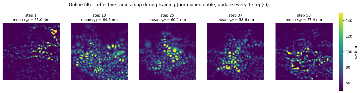
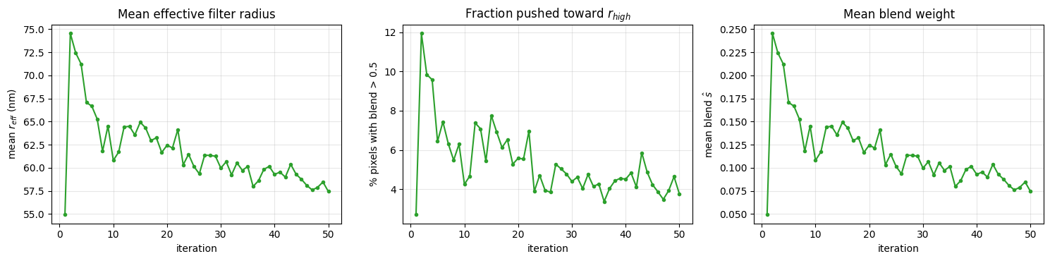
mean effective radius: 55.0 nm at step 1  ->  57.4 nm at step 50  (+2.5 nm)
blend map drift: mean |Δblend| between first and last snapshot = 0.0990
Evaluating the online device
CACHE_ONLINE_EVAL = RESULTS_DIR / f"wdm_online_{_tag}_eval.json"
SIM_ONLINE_EVAL   = SIMDATA_DIR  / f"online_{_tag}_eval.hdf5"

if CACHE_ONLINE_EVAL.exists() and SIM_ONLINE_EVAL.exists():
    eval_o = json.loads(CACHE_ONLINE_EVAL.read_text())
    sd_online = td.SimulationData.from_file(str(SIM_ONLINE_EVAL))
else:
    check_budget(1, "online eval", "forward", tag="eval")
    print("evaluating converged online device (1 simulation)")
    sim_eval = get_sim(params_online, beta=beta_final_o,
                       filter_fn=filter_online, include_extra_mnts=True)
    sd_online = web.run(sim_eval, task_name=f"wdm_online_{_tag}_eval",
                        path=str(SIM_ONLINE_EVAL), verbose=False)
    transmissions = []
    for i in range(num_freqs_design):
        amps = sd_online[mnts_mode[i].name].amps.sel(direction="+", mode_index=0)
        transmissions.append((np.abs(np.asarray(amps))**2).flatten().tolist())
    channel_metrics_o = [float(get_metric(sd_online, mnt_index=i, leak_weight=1.0))
                         for i in range(num_freqs_design)]
    eval_o = dict(
        channel_metrics = channel_metrics_o,
        physical_J = float(smooth_min(anp.array(channel_metrics_o))),
        transmissions = transmissions,
        channel_freqs = list(channel_freqs),
    )
    CACHE_ONLINE_EVAL.write_text(json.dumps(eval_o))
    print(f"saved {CACHE_ONLINE_EVAL}")

physical_J_o      = eval_o['physical_J']
channel_metrics_o = np.array(eval_o['channel_metrics'])

print("converged online device:")
print(f"  per-channel m_i: {channel_metrics_o}")
print(f"  physical J = smooth_min(m_i) = {physical_J_o:+.4f}    (training J was {o['Js'][-1]:+.4f})")
converged online device:
  per-channel m_i: [ 5.78506134e-01  7.78196927e-01  6.97293759e-01 -7.88584569e-05]
  physical J = smooth_min(m_i) = -0.9235    (training J was -1.2167)
# Fine-grid spectrum for the online device (1 simulation, 151 freqs).
CACHE_ONLINE_SPECTRUM = RESULTS_DIR / f"wdm_online_{_tag}_spectrum.json"
SIM_ONLINE_SPECTRUM   = SIMDATA_DIR  / f"online_{_tag}_spectrum.hdf5"

if CACHE_ONLINE_SPECTRUM.exists():
    spec_o = json.loads(CACHE_ONLINE_SPECTRUM.read_text())
else:
    check_budget(1, "online spectrum", "forward", tag="spectrum")
    print("computing fine-grid spectrum for online device (1 simulation, 151 freqs)")
    sim_spec = get_sim(params_online, beta=beta_final_o,
                       filter_fn=filter_online, include_extra_mnts=True)
    for i in range(num_freqs_design):
        sim_spec = sim_spec.updated_copy(freqs=list(freqs_measure), path=f"monitors/{i}")
        sim_spec = sim_spec.updated_copy(freqs=list(freqs_measure), path=f"monitors/{i + num_freqs_design}")
    sd_spec = web.run(sim_spec, task_name=f"wdm_online_{_tag}_spectrum",
                      path=str(SIM_ONLINE_SPECTRUM), verbose=False)
    powers_per_port = []
    for i in range(num_freqs_design):
        amps = sd_spec[mnts_mode[i].name].amps.sel(direction="+", mode_index=0)
        powers_per_port.append((np.abs(np.asarray(amps))**2).flatten().tolist())
    spec_o = dict(freqs_measure=list(freqs_measure), powers=powers_per_port)
    CACHE_ONLINE_SPECTRUM.write_text(json.dumps(spec_o))
    print(f"saved {CACHE_ONLINE_SPECTRUM}")
Schedule variant: refresh every $K$ steps, then freeze for the tail
The leading hypothesis for why the every-step online filter underperformed (see the Discussion) is that the gradient becomes edge-peaked as $\beta$ anneals. $\partial J/\partial\rho$ carries a $\mathrm{proj}' \sim \beta\,\mathrm{sech}^2(\beta(\rho-0.5))$ factor that concentrates on the material contour, increasingly so as $\beta$ ramps 1 → 50. Normalizing an edge-peaked field pushes blend → 1 on the boundary, which applies $r_{\rm high} = 150$ nm precisely where the optimizer is trying to resolve edges. If that is the mechanism, the damage is concentrated late in training, and the fix is simply to stop refreshing once $\beta$ is large.
This cell runs that test directly: refresh every SCHED_UPDATE_EVERY = 10 steps, and freeze the filter entirely for the final SCHED_FREEZE_LAST = 20 iterations. With 50 steps that means refreshes at steps 10, 20 and 30, then a fixed filter from step 31 to 50 — the whole high-$\beta$ phase runs on a filter that was chosen while $\beta$ was still moderate.
Three outcomes and what each would mean:
- Recovers most of the gap to the static run → hypothesis 1 is supported; late-training refresh is the problem and the schedule is the fix.
- Still far below static → the damage is not late-specific, pointing instead at the non-stationary-objective or geometry-jump hypotheses (2 and 3), which apply at every refresh regardless of $\beta$.
- Beats static → refreshing helps when it is confined to the phase where the design is still forming, which would be the most interesting result of the three.
Cost is one training run (~250 sims, ≈8.6 FlexUnits) plus two evaluation sims. That exceeds MAX_FLEX_UNITS = 3.0, so this cell is blocked by default and reports the estimate instead of dispatching. Raise the cap and set ALLOW_DISPATCH = True when you want it.
# --- schedule variant: refresh every K steps, frozen for the final N ---
SCHED_UPDATE_EVERY = 10
SCHED_FREEZE_LAST  = 20
_freeze_after      = num_steps - SCHED_FREEZE_LAST          # stop refreshing at this step index
_sched_tag         = f"{_tag}_k{SCHED_UPDATE_EVERY}_freeze{SCHED_FREEZE_LAST}"

CACHE_SCHED = RESULTS_DIR / f"wdm_online_{_sched_tag}_optim.json"

print(f"schedule: refresh every {SCHED_UPDATE_EVERY} steps up to step {_freeze_after}, "
      f"then frozen for the final {SCHED_FREEZE_LAST} "
      f"(beta at freeze ~ {beta_min + (beta_max-beta_min)*_freeze_after/(num_steps-1):.0f})")

if CACHE_SCHED.exists():
    sched = json.loads(CACHE_SCHED.read_text())
    print(f"cache hit: {CACHE_SCHED}")
else:
    try:
        filter_sched = make_online_adaptive_filter(
            radius_low=0.05, radius_high=0.15, dl=dl_design_region,
            alpha=1.0, mode=ONLINE_NORM, percentile=ONLINE_PERCENTILE)
        (_p, _J, _b, _pen, _bs, _bsn, _gp, _gd) = train_online(
            filter_sched, f"online-k{SCHED_UPDATE_EVERY}-freeze{SCHED_FREEZE_LAST}",
            seed_sensitivity=seed_field, update_every=SCHED_UPDATE_EVERY,
            snap_steps=BLEND_SNAP_STEPS, sens_wrt=SENS_WRT, freeze_after=_freeze_after)
        sched = dict(params_final=_p.tolist(), Js=_J, beta_history=_b,
                     penalty_history=_pen, blend_stats=_bs, blend_snapshots=_bsn,
                     sens_wrt=SENS_WRT,
                     sensitivity_field=np.asarray(_gd if SENS_WRT=="density" else _gp).tolist(),
                     final_blend=np.round(filter_sched.get_blend(), 4).tolist(),
                     update_every=int(SCHED_UPDATE_EVERY),
                     freeze_last=int(SCHED_FREEZE_LAST), freeze_after=int(_freeze_after),
                     normalization=ONLINE_NORM, percentile=float(ONLINE_PERCENTILE),
                     nx=int(nx), ny=int(ny))
        CACHE_SCHED.write_text(json.dumps(sched))
        print(f"saved {CACHE_SCHED}")
    except BudgetExceeded as e:
        sched = None
        print(e)
        print("\n  -> schedule variant not run. The comparison below reports the other devices only.")
schedule: refresh every 10 steps up to step 30, then frozen for the final 20 (beta at freeze ~ 31)
cache hit: misc/sens_aware_training/wdm_online_p99_density_k10_freeze20_optim.json
# Reconstruct the schedule device's geometry and its own sensitivity field.
# Both come straight out of the training cache -- NO simulations.
if sched is not None:
    params_sched   = np.array(sched['params_final'])
    beta_final_sch = sched['beta_history'][-1]
    filter_sched_final = make_online_adaptive_filter(
        radius_low=0.05, radius_high=0.15, dl=dl_design_region,
        alpha=1.0, mode=sched['normalization'], percentile=sched['percentile'])

    # CAREFUL: this run FREEZES the filter for its tail, so the map in force at the end
    # is the one set at the LAST REFRESH -- not the final gradient. Rebuilding from
    # `sensitivity_field` (the step-50 gradient) gives a different filter entirely
    # (measured: mean |Δblend| = 0.096, correlation 0.53), and therefore the wrong
    # geometry, eval and spectrum. Use the stored blend map itself.
    if sched.get('final_blend') is not None:
        _b_final = np.array(sched['final_blend'])
        _src = "final_blend"
    elif sched.get('blend_snapshots'):
        _snaps = sched['blend_snapshots']
        _b_final = np.array(_snaps[max(_snaps, key=int)])
        _src = f"blend snapshot at step {int(max(_snaps, key=int))+1}"
    else:
        raise RuntimeError("schedule cache has neither 'final_blend' nor 'blend_snapshots'; "
                           "cannot reconstruct the frozen filter state")
    filter_sched_final.set_blend(_b_final)
    print(f"  frozen filter reconstructed from {_src} (mean blend {_b_final.mean():.4f})")

    rho_sched = np.array(filter_sched_final(params_sched, beta=beta_final_sch))
    sensitivity_field_sched = np.abs(np.array(sched['sensitivity_field']))
    _side_sch, _n_sch = _smallest_feature_nm(rho_sched, dl_design_region)
    print(f"schedule device: {_n_sch} solid features, smallest ~{_side_sch:.0f} nm, "
          f"binarization {(rho_sched<0.05).mean()*100:.0f}% void / "
          f"{(rho_sched>0.95).mean()*100:.0f}% solid")
else:
    rho_sched = sensitivity_field_sched = None
  frozen filter reconstructed from blend snapshot at step 50 (mean blend 0.1155)
schedule device: 52 solid features, smallest ~15 nm, binarization 53% void / 42% solid
# Evaluate + fine-grid spectrum for the schedule device (2 sims, ~0.07 FU) so it can
# join the geometry, spectral and sensitivity comparisons. Cache-or-dispatch as usual.
eval_sched = spec_sched = None
if sched is not None:
    CACHE_SCHED_EVAL = RESULTS_DIR / f"wdm_online_{_sched_tag}_eval.json"
    SIM_SCHED_EVAL   = SIMDATA_DIR  / f"online_{_sched_tag}_eval.hdf5"
    CACHE_SCHED_SPEC = RESULTS_DIR / f"wdm_online_{_sched_tag}_spectrum.json"

    if CACHE_SCHED_EVAL.exists() and SIM_SCHED_EVAL.exists():
        eval_sched = json.loads(CACHE_SCHED_EVAL.read_text())
    else:
        try:
            check_budget(1, "schedule eval", "forward", tag="eval")
            _sim = get_sim(params_sched, beta=beta_final_sch,
                           filter_fn=filter_sched_final, include_extra_mnts=True)
            _sd = web.run(_sim, task_name=f"wdm_online_{_sched_tag}_eval",
                          path=str(SIM_SCHED_EVAL), verbose=False)
            _cm = [float(get_metric(_sd, mnt_index=i, leak_weight=1.0))
                   for i in range(num_freqs_design)]
            eval_sched = dict(channel_metrics=_cm,
                              physical_J=float(smooth_min(anp.array(_cm))))
            CACHE_SCHED_EVAL.write_text(json.dumps(eval_sched))
            print(f"saved {CACHE_SCHED_EVAL}")
        except BudgetExceeded as e:
            print(e)

    if CACHE_SCHED_SPEC.exists():
        spec_sched = json.loads(CACHE_SCHED_SPEC.read_text())
    else:
        try:
            check_budget(1, "schedule spectrum", "forward", tag="spectrum")
            _sim = get_sim(params_sched, beta=beta_final_sch,
                           filter_fn=filter_sched_final, include_extra_mnts=True)
            for i in range(num_freqs_design):
                _sim = _sim.updated_copy(freqs=list(freqs_measure), path=f"monitors/{i}")
                _sim = _sim.updated_copy(freqs=list(freqs_measure),
                                         path=f"monitors/{i + num_freqs_design}")
            _sd = web.run(_sim, task_name=f"wdm_online_{_sched_tag}_spectrum",
                          path=str(SIMDATA_DIR / f"online_{_sched_tag}_spectrum.hdf5"),
                          verbose=False)
            spec_sched = dict(freqs_measure=list(freqs_measure), powers=[
                (np.abs(np.asarray(_sd[mnts_mode[i].name].amps.sel(
                    direction="+", mode_index=0)))**2).flatten().tolist()
                for i in range(num_freqs_design)])
            CACHE_SCHED_SPEC.write_text(json.dumps(spec_sched))
            print(f"saved {CACHE_SCHED_SPEC}")
        except BudgetExceeded as e:
            print(e)

_SCHED_FULL = sched is not None and eval_sched is not None and spec_sched is not None
print(f"schedule device joins the full comparisons: {_SCHED_FULL}"
      + ("" if _SCHED_FULL else "  (trajectory-only without eval + spectrum)"))
schedule device joins the full comparisons: True
# Where the schedule variant lands, against everything else trained so far.
print(f"{'run':<44}{'final train J':>15}{'monotonic':>11}{'mean r_eff':>12}")
print("-" * 82)

def _row(label, hist, blend_stats=None):
    Jp = np.array(hist['Js']) + np.array(hist['penalty_history'])
    mono = 100 * np.mean(np.diff(Jp) > 0)
    r = (f"{np.mean([b['mean_r_eff_nm'] for b in blend_stats]):.1f} nm"
         if blend_stats else "fixed")
    print(f"{label:<44}{hist['Js'][-1]:>15.4f}{mono:>10.0f}%{r:>12}")

_row('uniform r=100nm', u)
_row('uniform r=50nm (control)', u50)
_row('sens-aware static (frozen, max-norm)', s)
_row('sens-aware online, every step', o, o.get('blend_stats'))
if sched is not None:
    _row(f'sens-aware online, every {SCHED_UPDATE_EVERY} + frozen last {SCHED_FREEZE_LAST}',
         sched, sched.get('blend_stats'))
    _gap_static = sched['Js'][-1] - s['Js'][-1]
    _gap_online = sched['Js'][-1] - o['Js'][-1]
    print()
    print(f"  vs static run       : {_gap_static:+.4f}")
    print(f"  vs every-step online: {_gap_online:+.4f}")
    _recovered = 100 * _gap_online / max(s['Js'][-1] - o['Js'][-1], 1e-9)
    print(f"  => freezing the tail recovers {_recovered:.0f}% of the gap between the "
          f"every-step online run and the static run.")
    print("     >70% supports the edge-peaked-gradient hypothesis; <30% points at the")
    print("     non-stationary-objective / geometry-jump hypotheses instead.")
else:
    print("\n  (schedule variant not run - see the budget message above)")
run                                           final train J  monotonic  mean r_eff
----------------------------------------------------------------------------------
uniform r=100nm                                     -0.7218        63%       fixed
uniform r=50nm (control)                            -0.6934        71%       fixed
sens-aware static (frozen, max-norm)                -0.6799        86%       fixed
sens-aware online, every step                       -1.2167        55%     61.7 nm
sens-aware online, every 10 + frozen last 20        -1.0051        82%     60.1 nm

  vs static run       : -0.3251
  vs every-step online: +0.2116
  => freezing the tail recovers 39% of the gap between the every-step online run and the static run.
     >70% supports the edge-peaked-gradient hypothesis; <30% points at the
     non-stationary-objective / geometry-jump hypotheses instead.
Comparison of all four devices
Every cross-device figure lives here, after all four training runs have completed:
| device | filter | role |
|---|---|---|
| uniform $r = 100$ nm | fixed radius | the original baseline (as submitted) |
| uniform $r = 50$ nm | fixed radius | control — matches the adaptive filter's floor |
| sens-aware static | $r \in [50,150]$ nm, one-shot map | the intervention |
| sens-aware online | $r \in [50,150]$ nm, refreshed each step | the intervention, per-iteration |
Which pairing answers which question. Baseline-vs-adaptive is the comparison originally reported, but it moves two variables at once. Control-vs-adaptive isolates sensitivity-driven reallocation, and it is the one to read for the mechanism. Static-vs-online isolates the refresh.
Training trajectories
All trained runs on one pair of axes. The schedule variant (refresh every $K$ steps, frozen for the tail) is drawn dashed with a vertical marker at the freeze point, so you can see directly whether its trajectory separates from the every-step online run after refreshing stops — which is what the edge-peaked-gradient hypothesis predicts. It appears in this figure only: without eval and spectrum simulations it cannot enter the geometry, spectral or robustness comparisons.
J_phys_o = np.array(o['Js']) + np.array(o['penalty_history'])

# ---- single registry driving every downstream comparison ----
DEV_COLORS = {'uniform': 'tab:blue', 'uniform50': 'tab:cyan',
              'sensaware': 'tab:purple', 'online': 'tab:green',
              'sched': 'tab:red'}
DEV_LABELS = {'uniform': 'uniform r=100nm', 'uniform50': 'uniform r=50nm (control)',
              'sensaware': 'sens-aware static', 'online': 'sens-aware online (every step)',
              'sched': f'sens-aware online (every {SCHED_UPDATE_EVERY}, frozen last {SCHED_FREEZE_LAST})'}
# Devices with a full data set (training + eval + spectrum) drive every figure.
COMPARE_DEVS = ['uniform', 'uniform50', 'sensaware', 'online']

TRAIN_HIST = {'uniform': u, 'uniform50': u50, 'sensaware': s, 'online': o}
SPECS      = {'uniform': spec_u, 'uniform50': spec_u50, 'sensaware': spec_s, 'online': spec_o}
PHYS_J     = {'uniform': physical_J_u, 'uniform50': physical_J_u50,
              'sensaware': physical_J_s, 'online': physical_J_o}
RHOS       = {'uniform': rho_uniform, 'uniform50': rho_uniform50,
              'sensaware': rho_sensaware, 'online': rho_online}

# The schedule variant joins every non-Monte-Carlo comparison once it has eval +
# spectrum; with training only it appears in the FoM trajectory plot alone. The MC/ED
# sections filter on data availability, so it drops out of those automatically.
if sched is not None:
    TRAIN_HIST['sched'] = sched
if _SCHED_FULL:
    COMPARE_DEVS.append('sched')
    SPECS['sched']  = spec_sched
    PHYS_J['sched'] = eval_sched['physical_J']
    RHOS['sched']   = rho_sched

TRAJ_DEVS = list(COMPARE_DEVS)
if sched is not None and 'sched' not in TRAJ_DEVS:
    TRAJ_DEVS.append('sched')
print(f"devices in the full comparisons : {COMPARE_DEVS}")
print(f"devices in the FoM trajectory   : {TRAJ_DEVS}")

def phys_traj(dev):
    """Physical-J trajectory = training J + penalty (penalty_weight = 1)."""
    h = TRAIN_HIST[dev]
    return np.array(h['Js']) + np.array(h['penalty_history'])

fig, axes = plt.subplots(1, 2, figsize=(14, 4.6), sharey=True)
for _key in TRAJ_DEVS:
    _phys, _train = phys_traj(_key), TRAIN_HIST[_key]['Js']
    _ls = '--' if _key == 'sched' else '-'
    axes[0].plot(its, _phys, marker='s', ms=3, ls=_ls, color=DEV_COLORS[_key],
                 label=f"{DEV_LABELS[_key]} → {_phys[-1]:+.3f}")
    axes[1].plot(its, _train, marker='o', ms=3, ls=_ls, color=DEV_COLORS[_key],
                 label=f"{DEV_LABELS[_key]} → {_train[-1]:+.3f}")
if sched is not None:
    # mark where the schedule variant stops refreshing
    for ax in axes:
        ax.axvline(_freeze_after + 1, color=DEV_COLORS['sched'], ls=':', lw=1.2, alpha=0.8)
    axes[0].annotate(f"filter frozen from step {_freeze_after+1}",
                     xy=(_freeze_after + 1, axes[0].get_ylim()[0]), fontsize=7,
                     color=DEV_COLORS['sched'], rotation=90,
                     va='bottom', ha='right')
axes[0].set_ylabel('J'); axes[0].set_title("Physical J = smooth_min(channels), no penalty")
axes[1].set_title("Training J = physical J − penalty")
for ax in axes:
    ax.set_xlabel('iteration'); ax.legend(loc='lower right', fontsize=7); ax.grid(alpha=0.3)
plt.tight_layout()
plt.show()

def _monotonicity(arr):
    return float(np.mean(np.diff(np.asarray(arr, dtype=float)) > 0))

print("physical J at convergence / fraction of strictly-improving steps:")
for _key in TRAJ_DEVS:
    _phys = phys_traj(_key)
    if _key not in PHYS_J:      # trajectory-only device (no eval sim)
        print(f"  {DEV_LABELS[_key]:<52} train-end {_phys[-1]:+.4f}   "
              f"eval     n/a   monotonic {100*_monotonicity(_phys):.0f}%")
        continue
    print(f"  {DEV_LABELS[_key]:<52} train-end {_phys[-1]:+.4f}   "
          f"eval {PHYS_J[_key]:+.4f}   monotonic {100*_monotonicity(_phys):.0f}%")

print("\n--- the control comparison (eval physical J) ---")
_d_freedom = PHYS_J['uniform50'] - PHYS_J['uniform']
_d_static  = PHYS_J['sensaware'] - PHYS_J['uniform50']
_d_online  = PHYS_J['online']    - PHYS_J['uniform50']
_d_total   = PHYS_J['sensaware'] - PHYS_J['uniform']
print(f"  finer floor alone   (u50 − u100)      : {_d_freedom:+.4f}")
print(f"  static reallocation (static − u50)    : {_d_static:+.4f}")
print(f"  online reallocation (online − u50)    : {_d_online:+.4f}")
if 'sched' in PHYS_J:
    print(f"  schedule variant    (sched − u50)     : {PHYS_J['sched'] - PHYS_J['uniform50']:+.4f}")
    print(f"  schedule vs every-step online         : {PHYS_J['sched'] - PHYS_J['online']:+.4f}")
print(f"  total static gain   (static − u100)   : {_d_total:+.4f}")
if abs(_d_total) > 1e-9:
    print(f"\n  share of the reported static gain attributable to the finer floor alone: "
          f"{100*_d_freedom/_d_total:.0f}%")
    print(f"  share attributable to sensitivity-driven reallocation:                    "
          f"{100*_d_static/_d_total:.0f}%")
devices in the full comparisons : ['uniform', 'uniform50', 'sensaware', 'online', 'sched']
devices in the FoM trajectory   : ['uniform', 'uniform50', 'sensaware', 'online', 'sched']
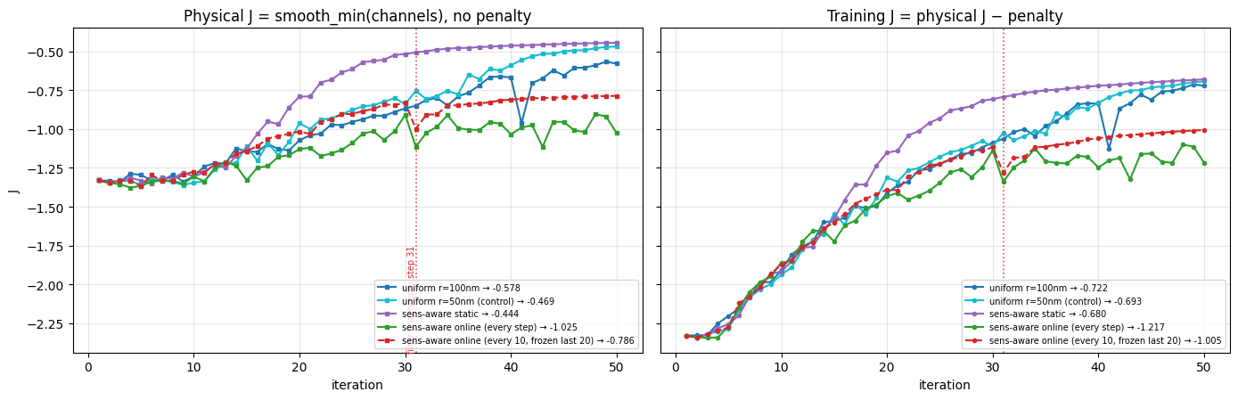
physical J at convergence / fraction of strictly-improving steps:
  uniform r=100nm                                      train-end -0.5785   eval -0.5565   monotonic 63%
  uniform r=50nm (control)                             train-end -0.4687   eval -0.4678   monotonic 71%
  sens-aware static                                    train-end -0.4438   eval -0.4424   monotonic 86%
  sens-aware online (every step)                       train-end -1.0248   eval -0.9235   monotonic 55%
  sens-aware online (every 10, frozen last 20)         train-end -0.7861   eval -0.7846   monotonic 82%

--- the control comparison (eval physical J) ---
  finer floor alone   (u50 − u100)      : +0.0888
  static reallocation (static − u50)    : +0.0254
  online reallocation (online − u50)    : -0.4557
  schedule variant    (sched − u50)     : -0.3168
  schedule vs every-step online         : +0.1389
  total static gain   (static − u100)   : +0.1141

  share of the reported static gain attributable to the finer floor alone: 78%
  share attributable to sensitivity-driven reallocation:                    22%
Geometry
Initial state plus all four converged designs, with feature counts and the smallest solid feature in each. Pixel-flip percentages are quoted against the $r = 50$ nm control, since that is the meaningful reference for the adaptive filters.
sim_online_final    = get_sim(params_online, beta=beta_final_o,
                              filter_fn=filter_online, include_extra_mnts=False)
sim_uniform50_final = get_sim(params_uniform50, beta=beta_final_u50,
                              filter_fn=filter_uniform50, include_extra_mnts=False)
SIMS_FINAL = {'uniform': sim_uniform_final, 'uniform50': sim_uniform50_final,
              'sensaware': sim_sensaware_final, 'online': sim_online_final}
if 'sched' in COMPARE_DEVS:
    # built from the density directly -- constructing a Simulation dispatches nothing
    SIMS_FINAL['sched'] = get_sim_from_density(rho_sched, include_extra_mnts=False)

FEATURES = {d: _smallest_feature_nm(RHOS[d], dl_design_region) for d in COMPARE_DEVS}

_panels = [('init', sim_init, "Init  (ρ = 0.5, β = β₀)")] + [
    (d, SIMS_FINAL[d], f"{DEV_LABELS[d]}\n{FEATURES[d][1]} features, "
                       f"smallest ~{FEATURES[d][0]:.0f} nm") for d in COMPARE_DEVS]

fig, axes = plt.subplots(1, len(_panels), figsize=(3.9 * len(_panels), 4.6))
for ax, (_key, _sim, _title) in zip(np.atleast_1d(axes), _panels):
    _sim.plot_eps(z=0.01, ax=ax, monitor_alpha=0, source_alpha=0)
    ax.set_title(_title, fontsize=9)
    ax.set_aspect('equal')
plt.tight_layout()
plt.show()

print(f"{'device':<28}{'features':>10}{'smallest':>12}   pixel flips vs control (u50)")
for _key in COMPARE_DEVS:
    _side, _n = FEATURES[_key]
    _flip = ((RHOS['uniform50'] > 0.5) != (RHOS[_key] > 0.5)).mean() * 100
    print(f"  {DEV_LABELS[_key]:<26}{_n:>10}{_side:>9.0f} nm{_flip:>22.0f}%")

device                        features    smallest   pixel flips vs control (u50)
  uniform r=100nm                   29      113 nm                    32%
  uniform r=50nm (control)          56       95 nm                     0%
  sens-aware static                 50      103 nm                    18%
  sens-aware online (every step)        39       75 nm                    24%
  sens-aware online (every 10, frozen last 20)        52       15 nm                    23%
Spectra
Per-port transmission for all four devices on the 151-point fine grid, linear (top) and dB (bottom), with the in-band mean per port tabulated underneath. The original writeup's claim was that the adaptive spectrum sits at or above the baseline across the whole bandwidth — check that against the $r = 50$ nm control curve, not just the $r = 100$ nm one.
# Per-port spectra, all four devices.
fig, axes = plt.subplots(2, num_freqs_design, figsize=(16, 7), sharex=True)
for i in range(num_freqs_design):
    fmin, fmax = channel_bounds[i]
    idx = int(np.argmin(np.abs(freqs_cmp - float(freqs_design[i]))))
    for row, (_transform, _ylabel) in enumerate([
            (lambda p: p * 100,                              'transmission (%)'),
            (lambda p: 10*np.log10(np.maximum(p, 1e-6)),      'transmission (dB)')]):
        ax = axes[row, i]
        ax.axvspan(1000 * td.C_0 / fmin, 1000 * td.C_0 / fmax, alpha=0.15, color='gray')
        for _key in COMPARE_DEVS:
            _y = _transform(np.array(SPECS[_key]['powers'][i]))
            ax.plot(wvls_cmp, _y, color=DEV_COLORS[_key], label=DEV_LABELS[_key], lw=1.2)
            ax.scatter([wvls_design[i]*1e3], [_y[idx]], 45, marker='*',
                       color=DEV_COLORS[_key], zorder=5)
        ax.axvline(wvls_design[i]*1e3, color='gray', ls=':', alpha=0.5)
        ax.grid(alpha=0.3)
        if row == 0:
            ax.set_title(f"port {i} (design {wvls_design[i]*1e3:.0f} nm)")
            ax.set_ylim(0, 100)
        else:
            ax.set_xlabel('wavelength (nm)')
        if i == 0:
            ax.set_ylabel(_ylabel)
            if row == 1:
                ax.legend(fontsize=6.5, loc='lower right')
fig.suptitle("Per-port transmission spectra — baseline, control, and both adaptive filters", y=1.00)
plt.tight_layout()
plt.show()

# In-band mean transmission per port, all four devices.
_inband = [(freqs_cmp >= channel_bounds[i][0]) & (freqs_cmp <= channel_bounds[i][1])
           for i in range(num_freqs_design)]
print("in-band mean transmission per port (%):")
print(f"  {'device':<28}" + "".join(f"port {i:<6}" for i in range(num_freqs_design)) + "    mean")
for _key in COMPARE_DEVS:
    _vals = [100 * np.array(SPECS[_key]['powers'][i])[_inband[i]].mean()
             for i in range(num_freqs_design)]
    print(f"  {DEV_LABELS[_key]:<28}" + "".join(f"{v:>9.1f}  " for v in _vals)
          + f"{np.mean(_vals):>8.1f}")
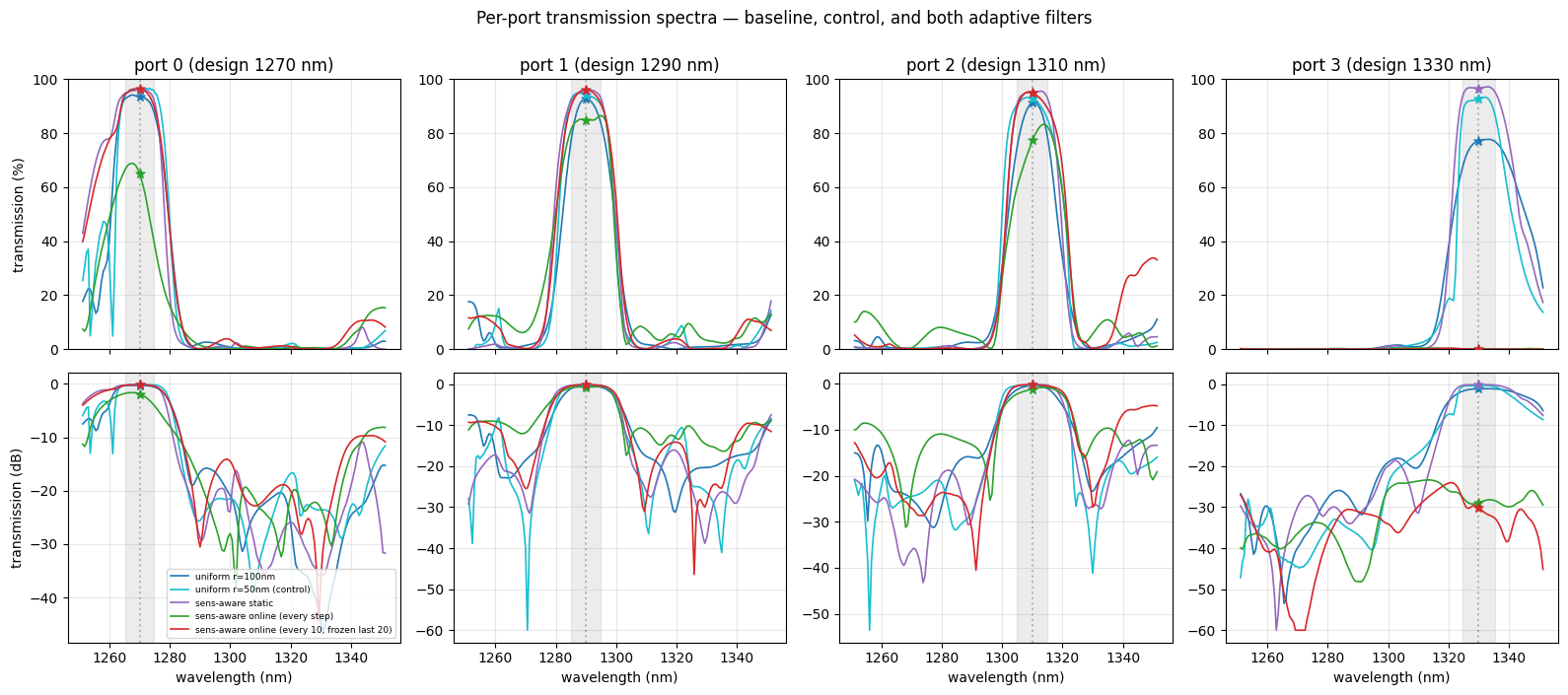
in-band mean transmission per port (%):
  device                      port 0     port 1     port 2     port 3         mean
  uniform r=100nm                  92.9       89.1       86.6       75.9      86.1
  uniform r=50nm (control)         96.1       93.7       91.2       91.9      93.2
  sens-aware static                95.5       94.9       94.7       96.6      95.4
  sens-aware online (every step)     60.8       84.8       75.4        0.1      55.3
  sens-aware online (every 10, frozen last 20)     95.2       94.5       93.3        0.1      70.8
Sensitivity
Two complementary views, both now spanning every device.
Figure 1 — routing against the original hot spots. All four contours drawn on the same background: the uniform-$r{=}100$ design's sensitivity field, which is the map that drove the static adaptive filter. This is the direct test of the geometric mechanism — did the adaptive designs route their boundaries around the bright pixels? The $r = 50$ nm control is the reference: it saw the same design problem with the same floor but no sensitivity information, so any routing difference between it and the adaptive designs is attributable to the filter rather than to feature size.
Figure 2 — each design on its own field. Where sensitivity sits after each run converged. Read this with the caveat below.
# Figure 1: every contour on the uniform-design sensitivity field (the map that drove the filter).
_vmax_uniform_field = sensitivity_field.max()

fig, axes = plt.subplots(1, len(COMPARE_DEVS), figsize=(4.2 * len(COMPARE_DEVS), 4.6))
for ax, _key in zip(np.atleast_1d(axes), COMPARE_DEVS):
    im = ax.imshow(np.flipud(sensitivity_field.T), cmap='magma',
                   vmin=0, vmax=_vmax_uniform_field)
    ax.contour(np.flipud(RHOS[_key].T), levels=[0.5], colors='white', linewidths=0.5)
    ax.set_title(f"+ {DEV_LABELS[_key]} contour", fontsize=9)
    ax.axis('off')
fig.colorbar(im, ax=axes, fraction=0.02, pad=0.02, label=r'$|\partial J / \partial \rho|$')
fig.suptitle(r"Uniform-$r{=}100$nm sensitivity field $|\partial J/\partial\rho|$ "
             r"with each converged contour  "
             f"(range = {_rng_u:.2e}, mean = {_mean_u:.2e})", fontsize=11)
plt.show()

# How much of each design's boundary sits in the top-decile sensitivity region?
_hot = sensitivity_field >= np.percentile(sensitivity_field, 90)
print("fraction of each design's material boundary lying in the top-decile "
      "sensitivity region of the uniform field:")
for _key in COMPARE_DEVS:
    _b = np.abs(np.gradient((RHOS[_key] > 0.5).astype(float))).sum(axis=0) > 0
    print(f"  {DEV_LABELS[_key]:<28}{100 * (_b & _hot).sum() / max(_b.sum(), 1):>6.1f}%")
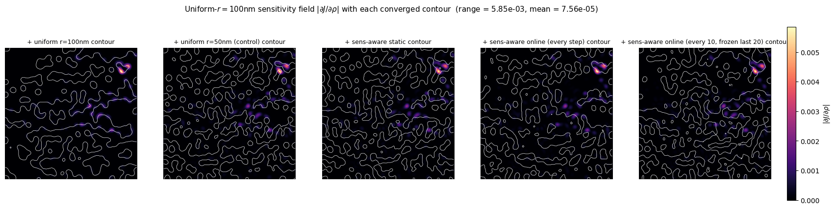
fraction of each design's material boundary lying in the top-decile sensitivity region of the uniform field:
  uniform r=100nm               22.0%
  uniform r=50nm (control)      11.3%
  sens-aware static             11.0%
  sens-aware online (every step)  10.6%
  sens-aware online (every 10, frozen last 20)  12.2%
# Online design's own sensitivity field (cache-or-dispatch: 1 forward+adjoint sim).
# Stores both variables so the figures can be drawn in whichever one SENS_WRT selects.
ONLINE_SENS_CACHE = RESULTS_DIR / f"online_{_tag}_sensitivity.json"
if ONLINE_SENS_CACHE.exists():
    _online_sens_data = json.loads(ONLINE_SENS_CACHE.read_text())
    print(f"loaded {ONLINE_SENS_CACHE}")
else:
    check_budget(1 + num_freqs_design, "online sensitivity", "forward", tag="sensitivity")
    print("online sensitivity cache missing — computing one forward+adjoint sim")
    _val_o, _gp_o, _gd_o = value_and_grads(params_online, beta=beta_final_o,
                                           filter_fn=filter_online,
                                           penalty_weight=1.0, leak_weight=1.0)
    _online_sens_data = dict(sensitivity_params=np.asarray(_gp_o).tolist(),
                             sensitivity_density=np.asarray(_gd_o).tolist(),
                             nx=int(nx), ny=int(ny))
    ONLINE_SENS_CACHE.write_text(json.dumps(_online_sens_data))
    print(f"saved {ONLINE_SENS_CACHE}")

# The comparison figures use one variable consistently across devices. Only the online
# run has dJ/d(rho_bar) for free; the three earlier devices only ever persisted
# dJ/d(rho), so the figures fall back to dJ/d(rho) unless every device has the other.
_online_key = ('sensitivity_density' if SENS_WRT == 'density'
                                        and 'sensitivity_density' in _online_sens_data
               else 'sensitivity_params')
if _online_key not in _online_sens_data:                     # pre-fix cache layout
    _online_key = 'sensitivity_field'
sensitivity_field_online = np.abs(np.array(_online_sens_data[_online_key]))
SENS_FIGURE_VAR = r'\partial J/\partial\rho'
print(f"sensitivity figures drawn in: dJ/d(rho)   [the three earlier devices only have "
      f"this variable; the online run's dJ/d(rho_bar) is cached alongside]")

SENS_FIELDS = {'uniform': sensitivity_field, 'uniform50': sensitivity_field_uniform50,
               'sensaware': sensitivity_field_sensaware, 'online': sensitivity_field_online}
if 'sched' in COMPARE_DEVS:
    SENS_FIELDS['sched'] = sensitivity_field_sched
SENS_STATS  = {d: _sens_stats(SENS_FIELDS[d]) for d in COMPARE_DEVS}
_vmax_all   = max(f.max() for f in SENS_FIELDS.values())

fig, axes = plt.subplots(1, len(COMPARE_DEVS), figsize=(4.4 * len(COMPARE_DEVS), 5.0))
for ax, _key in zip(np.atleast_1d(axes), COMPARE_DEVS):
    _rng, _mean = SENS_STATS[_key]
    im = ax.imshow(np.flipud(SENS_FIELDS[_key].T), cmap='magma', vmin=0, vmax=_vmax_all)
    ax.contour(np.flipud(RHOS[_key].T), levels=[0.5], colors='white', linewidths=0.5)
    ax.set_title(f"{DEV_LABELS[_key]}\nrange = {_rng:.2e},  mean = {_mean:.2e}", fontsize=9)
    ax.axis('off')
fig.colorbar(im, ax=axes, fraction=0.02, pad=0.02, label=r'$|\partial J / \partial \rho|$')
fig.suptitle("Each design on its own sensitivity field — shared color scale", fontsize=12)
plt.show()

print("own-sensitivity statistics (see the caveat above — these are illustrative, not confirmatory):")
for _key in COMPARE_DEVS:
    _rng, _mean = SENS_STATS[_key]
    print(f"  {DEV_LABELS[_key]:<28} range = {_rng:.3e}   mean = {_mean:.3e}")
loaded misc/sens_aware_training/online_p99_density_sensitivity.json
sensitivity figures drawn in: dJ/d(rho)   [the three earlier devices only have this variable; the online run's dJ/d(rho_bar) is cached alongside]
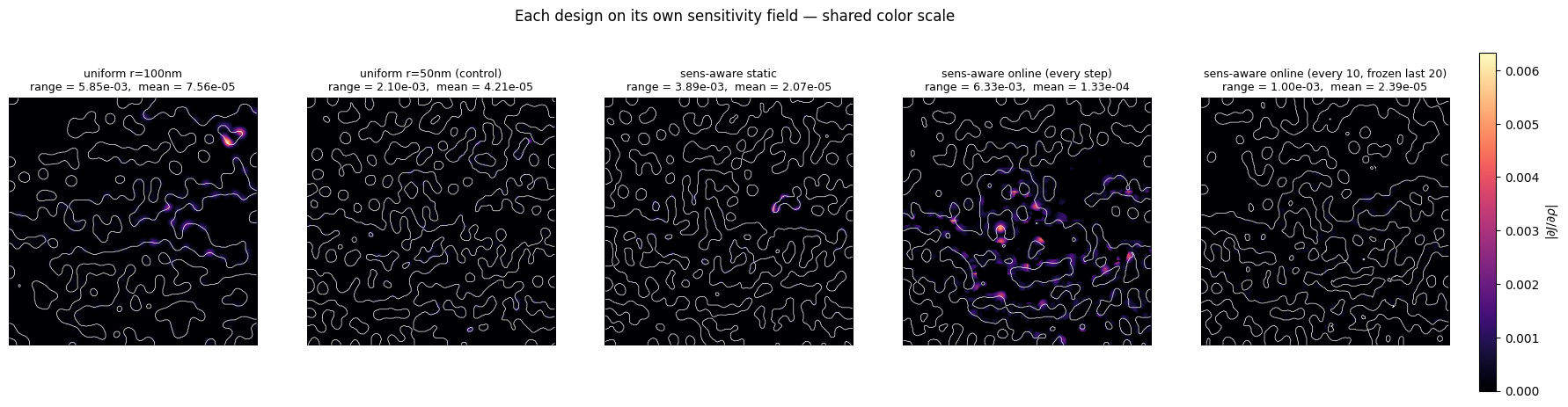
own-sensitivity statistics (see the caveat above — these are illustrative, not confirmatory):
  uniform r=100nm              range = 5.848e-03   mean = 7.558e-05
  uniform r=50nm (control)     range = 2.104e-03   mean = 4.211e-05
  sens-aware static            range = 3.890e-03   mean = 2.074e-05
  sens-aware online (every step) range = 6.332e-03   mean = 1.329e-04
  sens-aware online (every 10, frozen last 20) range = 1.000e-03   mean = 2.389e-05
Reading this section.
Training trajectories. The printout splits the reported static gain into what the finer floor buys on its own (uniform r=50nm − uniform r=100nm) and what sensitivity-driven reallocation adds on top (static − uniform r=50nm). The second number is the only part attributable to the mechanism this notebook is about; the headline baseline comparison bundles both.
Geometry. If the $r = 50$ nm control produces a similar smallest-feature size to the adaptive devices, the adaptive filter's coarsening in high-sensitivity regions is not actually binding — which is what the near-uniform blend map measured in the diagnostic above would predict.
Sensitivity, Figure 1. The boundary-in-hot-region percentages under the figure quantify what was previously an eyeball judgement. The claim in the original writeup was that the sens-aware design routes around the bright pixels; that claim is only supported if the adaptive designs score meaningfully lower than the $r = 50$ nm control, not merely lower than the $r = 100$ nm baseline — a finer floor changes boundary length and therefore this statistic on its own.
Sensitivity, Figure 2. Suggestive, not confirmatory, and we do not lean on it. Gradient magnitude falls as an optimization approaches a stationary point, and the runs converged to different $J$ — so a smaller $|\partial J/\partial\rho|$ is partly a signature of being further along, not independent evidence of robustness. The fields also inherit the scale of their own $J$, so they are not strictly on a common scale. Reading "lower sensitivity ⟹ more robust" straight off these panels would be circular. The load-bearing robustness evidence is the Monte-Carlo data below, which measures actual FoM degradation under actual perturbations.
Robustness under fabrication constraints
We compare the two converged designs under three fabrication-noise models, each varying along its own amplitude axis:
- CD jitter — independent per-pixel Gaussian noise on the converged density. Random edge-position errors uniformly distributed across the design region.
- Microloading + proximity effect — feature-size-dependent random morphological dilation/erosion. Smaller features get larger random per-feature deltas; large features stay close to nominal.
- Uniform erosion / dilation — a deterministic, spatially-uniform global boundary shift modeling lithography bias and CDU drift.
For (1) and (2) we sweep 17 amplitude ratios [0.1, 0.2, 0.3, 0.5, 0.7, 1, 1.5, 2, 2.5, 3, 3.5, 4, 4.5, 5, 10, 20, 50] (a fine ladder near zero, a 0.5-spaced ladder through the crossover region, and a coarse ladder out to large amplitudes), with 30 random seeds per amplitude per device — 1020 sims per noise model. For (3) we sweep 11 amounts $\Delta \in \{-10, -8, -6, -4, -2, 0, +2, +4, +6, +8, +10\}\;\mathrm{nm}$, 22 sims total. All sims use the corrected builder (design-region mesh override + 151-freq fine-grid monitors); $\Delta = 0$ in (3) short-circuits the SDF-tanh re-rasterization so it sits exactly on the noise-free eval baseline.
Caveat — microloading binarization residual.
apply_microloading_proximityre-binarizes the converged density viarho > 0.5before applying per-feature morphological deltas. At small amplitudes (where the per-feature sigma is too small for any delta to round to ±1 pixel), all 30 seeds reduce to the same binarized design. That binarized design's FoM differs slightly from the original (smooth-near-binary)rho's eval baseline — sens-aware loses ~3% from this residual, uniform <1%. The relative comparison between the two designs is unaffected.
from scipy import ndimage

# === perturbed-sim builder (shared across all noise models) ===

# Fine-grid frequencies (matches the noise-free spectrum eval at 151 points).
# Reused by the cache-or-dispatch fallbacks below, so perturbed-sim mode/flux
# monitors record at the same wavelengths as the eval baseline.
num_freqs_measure = 151
freqs_measure = list(np.linspace(freq_min - df_design, freq_max + df_design, num_freqs_measure))


def _build_perturbed_sim(rho_perturbed, fine_freqs=None):
    """Build a Simulation that runs FDTD on a perturbed density.

    Always adds the design-region MeshOverrideStructure (15 nm grid) so the FoM
    matches the noise-free eval pipeline. If `fine_freqs` is given, the mode
    and flux monitors are re-emitted on that frequency grid (e.g. the 151-pt
    spectrum grid). Otherwise the static-sim monitor frequencies are kept.
    """
    rho_clipped = np.clip(rho_perturbed, 0, 1).astype(np.float64)
    eps_field = (n_air**2 + (n_si**2 - n_air**2) * rho_clipped).reshape((nx, ny, 1))
    xs = np.linspace(-lx/2, lx/2, nx)
    ys = np.linspace(-ly/2, ly/2, ny)
    coords = dict(x=xs, y=ys, z=[0])
    eps_arr = td.ScalarFieldDataArray(data=eps_field, coords=coords)
    medium = td.CustomMedium(permittivity=eps_arr)
    structure = td.Structure(geometry=design_region_geo, medium=medium)
    override = td.MeshOverrideStructure(
        geometry=design_region_geo, dl=[dl_design_region]*3,
    )
    grid_spec = sim_static.grid_spec.updated_copy(
        override_structures=list(sim_static.grid_spec.override_structures) + [override]
    )
    sim = sim_static.updated_copy(
        structures=list(sim_static.structures) + [structure],
        grid_spec=grid_spec,
    )
    if fine_freqs is not None:
        new_mnts = []
        for m in sim.monitors:
            if isinstance(m, (td.ModeMonitor, td.FluxMonitor)):
                new_mnts.append(m.updated_copy(freqs=list(fine_freqs)))
            else:
                new_mnts.append(m)
        sim = sim.updated_copy(monitors=new_mnts)
    return sim


# === per-pixel Gaussian density noise (CD jitter) ===
def apply_cd_jitter(rho_clean, sigma, rng):
    return np.clip(rho_clean + rng.normal(0.0, sigma, rho_clean.shape), 0.0, 1.0)


# === per-feature random morphological dilation/erosion (microloading + proximity) ===
def apply_microloading_proximity(rho_clean, amplitude, rng):
    binary = (rho_clean > 0.5)
    labels, n_features = ndimage.label(binary)
    if n_features == 0:
        return rho_clean.copy()
    feature_sizes      = np.bincount(labels.ravel())[1:]
    feature_diameters  = 2.0 * np.sqrt(feature_sizes / np.pi)
    sigmas             = amplitude / np.maximum(feature_diameters, 2.0)
    deltas             = rng.normal(0.0, sigmas)
    deltas             = np.clip(deltas, -30, 30)
    rho_perturbed = binary.astype(np.float64).copy()
    for label_id in range(1, n_features + 1):
        d = int(round(deltas[label_id - 1]))
        if abs(d) < 1:
            continue
        feature_mask = (labels == label_id)
        if d > 0:
            new_mask = ndimage.binary_dilation(feature_mask, iterations=d)
        else:
            new_mask = ndimage.binary_erosion(feature_mask,  iterations=-d)
        rho_perturbed[feature_mask & ~new_mask] = 0.0
        rho_perturbed[~feature_mask & new_mask] = 1.0
    return rho_perturbed
# === noise-free reference spectra and baselines (151 fine-grid freqs) ===
# The ED sweep monitors at the same 151-point grid as the eval spectrum, so we use
# the cached fine-grid spectra (rather than the 20-freq eval json) to compute the
# baseline FoM and the dashed reference curves used by the ED spectra plot.
spec_u_full = json.loads((RESULTS_DIR / 'wdm_uniform_spectrum.json').read_text())
spec_s_full = json.loads((RESULTS_DIR / 'wdm_sensaware_spectrum.json').read_text())

ref_freqs   = np.array(spec_u_full['freqs_measure'])      # (151,)
ref_T_full = {
    'uniform':   np.array(spec_u_full['powers']),         # (4 ports, 151 freqs)
    'sensaware': np.array(spec_s_full['powers']),
}

def baseline_sum_from_spectrum(powers_4xN, freqs_N):
    """Sum of per-channel m_i = T_{i,band_i} - mean_{j!=i} T_{i,band_j}, computed on 151-freq data."""
    n = num_freqs_design
    T = np.zeros((n, n))
    for port in range(n):
        for band in range(n):
            in_band = (freqs_N >= channel_bounds[band][0]) & (freqs_N <= channel_bounds[band][1])
            T[port, band] = powers_4xN[port, in_band].mean()
    m = np.array([T[i, i] - sum(T[i, j] for j in range(n) if j != i) / (n - 1)
                  for i in range(n)])
    return float(m.sum())

baseline_u = baseline_sum_from_spectrum(ref_T_full['uniform'],   ref_freqs)
baseline_s = baseline_sum_from_spectrum(ref_T_full['sensaware'], ref_freqs)
print(f"noise-free baselines (151-freq metric):  uniform={baseline_u:+.4f}   sens-aware={baseline_s:+.4f}")
noise-free baselines (151-freq metric): uniform=+3.3987 sens-aware=+3.8068
CD jitter and microloading (stochastic noise models)
Each MC cell (noise model, device, amplitude) averages 30 random seeds. We first show the box-and-whisker distribution of $\sum_i m_i$ per cell (with the noise-free baseline as a dashed reference), then a representative perturbed design at one seed per cell, and finally the mean per-port transmission spectrum across the 30 seeds at the 151-point fine grid.
# === MC sweep config ===
# Target sweep: a coarse ladder (0.1..0.7, 1, 3, 10, 20, 50) plus a fine
# 1..5-by-0.5 ladder. If the cached files contain only a subset of these
# ratios, plots render that subset; only when caches are entirely absent
# does the dispatch fallback below run on the full target list.
RATIOS_TARGET = sorted({0.1, 0.2, 0.3, 0.5, 0.7,
                        1, 1.5, 2, 2.5, 3, 3.5, 4, 4.5, 5,
                        10, 20, 50})
N_SAMPLES = 30
BASE_SEED = 0

CD_JITTER_BASE        = 0.01
MICROLOADING_BASE       = 1.0

CACHE_CD_U = RESULTS_DIR / "mc_cdjitter_uniform.json"
CACHE_CD_S = RESULTS_DIR / "mc_cdjitter_sensaware.json"
CACHE_ML_U = RESULTS_DIR / "mc_microloading_uniform.json"
CACHE_ML_S = RESULTS_DIR / "mc_microloading_sensaware.json"
CACHE_MC_SPECTRA = RESULTS_DIR / "mc_spectra.json"

_caches_exist = all(p.exists() for p in
                    [CACHE_CD_U, CACHE_CD_S, CACHE_ML_U, CACHE_ML_S, CACHE_MC_SPECTRA])

if _caches_exist:
    mc_cd_u = json.loads(CACHE_CD_U.read_text())
    mc_cd_s = json.loads(CACHE_CD_S.read_text())
    mc_ml_u = json.loads(CACHE_ML_U.read_text())
    mc_ml_s = json.loads(CACHE_ML_S.read_text())
    mc_spec = json.loads(CACHE_MC_SPECTRA.read_text())

    # Use whatever amplitudes are present in BOTH device caches and BOTH MC types,
    # so CD and ML plots stay aligned even if one MC type is partway through dispatch.
    # Iterate target ratios and check key presence by f'{amp:g}' string (robust to
    # floating-point precision in BASE*ratio arithmetic).
    def _ratio_present(r):
        cd_key = f"{CD_JITTER_BASE   * r:g}"
        ml_key = f"{MICROLOADING_BASE * r:g}"
        return (cd_key in mc_cd_u and cd_key in mc_cd_s
                and ml_key in mc_ml_u and ml_key in mc_ml_s)
    _common_ratios = [r for r in RATIOS_TARGET if _ratio_present(r)]
    RATIOS = _common_ratios
    CD_JITTER_AMPLITUDES    = [CD_JITTER_BASE   * r for r in RATIOS]
    MICROLOADING_AMPLITUDES = [MICROLOADING_BASE * r for r in RATIOS]
    print(f"loaded MC caches: using {len(RATIOS)} common ratios (CD has {len(mc_cd_u)} amps, "
          f"ML has {len(mc_ml_u)} amps in cache).")
    if set(RATIOS) != set(RATIOS_TARGET):
        _missing = sorted(set(RATIOS_TARGET) - set(RATIOS))
        print(f"  note: {len(_missing)} target ratio(s) not yet in cache: {_missing}.")
        print("  delete the MC cache JSONs and re-execute this cell to dispatch the full sweep.")
    print(f"loaded MC caches: {len(mc_cd_u)} CD amps, {len(mc_ml_u)} ML amps, "
          f"{len(mc_spec['cells'])} mean spectra")
else:
    # No caches found at all — dispatch the full target sweep from scratch.
    RATIOS = list(RATIOS_TARGET)
    CD_JITTER_AMPLITUDES    = [CD_JITTER_BASE   * r for r in RATIOS]
    MICROLOADING_AMPLITUDES = [MICROLOADING_BASE * r for r in RATIOS]
    _cd_missing_u = list(CD_JITTER_AMPLITUDES)
    _cd_missing_s = list(CD_JITTER_AMPLITUDES)
    _ml_missing_u = list(MICROLOADING_AMPLITUDES)
    _ml_missing_s = list(MICROLOADING_AMPLITUDES)
    print(f"MC caches missing — dispatching full target sweep "
          f"({len(RATIOS)} amps × 30 seeds × 2 devices × 2 noise types = "
          f"{len(RATIOS) * 30 * 2 * 2} sims).")

    mc_cd_u, mc_cd_s, mc_ml_u, mc_ml_s = {}, {}, {}, {}
    mc_spec = dict(freqs=None, cells={})

    import time
    from collections import defaultdict
    _mc_dir = SIMDATA_DIR / "mc_dispatch"; _mc_dir.mkdir(exist_ok=True)

    def _build_mc_batch_per_dev(perturb_fn, mc_label, missing_per_dev):
        """Build sims for a list of (device, amplitudes) pairs."""
        sims, idx = {}, {}
        for rho, dev, amps in missing_per_dev:
            rho_np = np.asarray(rho, dtype=float)
            for amp in amps:
                for seed in range(BASE_SEED, BASE_SEED + N_SAMPLES):
                    rng = np.random.default_rng(seed)
                    rho_p = perturb_fn(rho_np, amp, rng)
                    task = f"hack_{mc_label}_{dev}_amp{amp:g}_seed{seed}"
                    sims[task] = _build_perturbed_sim(rho_p, fine_freqs=freqs_measure)
                    idx[task]  = (mc_label, dev, amp, seed)
        return sims, idx

    def _robust_run(sims, label, max_retries=5):
        delay = 60
        for attempt in range(1, max_retries + 1):
            try:
                return web.run_async(sims, path_dir=str(_mc_dir), verbose=True)
            except Exception as e:
                msg = str(e)[:150]
                print(f"[{label}] attempt {attempt} failed: {msg}")
                if attempt == max_retries:
                    raise
                print(f"[{label}] sleeping {delay}s before retry...")
                time.sleep(delay)
                delay = min(delay * 2, 600)

    cd_missing_per_dev = [(rho_uniform, "uniform", _cd_missing_u),
                          (rho_sensaware, "sensaware", _cd_missing_s)]
    ml_missing_per_dev = [(rho_uniform, "uniform", _ml_missing_u),
                          (rho_sensaware, "sensaware", _ml_missing_s)]

    check_budget(len(_cd_missing_u) + len(_cd_missing_s) + len(_ml_missing_u) + len(_ml_missing_s),
                 "MC sweep (uniform + sens-aware)", "perturbed", tag="mc")
    print("=== building CD jitter sims (missing only) ===")
    cd_sims, cd_idx = _build_mc_batch_per_dev(apply_cd_jitter, "cdjitter", cd_missing_per_dev)
    print("=== building microloading sims (missing only) ===")
    ml_sims, ml_idx = _build_mc_batch_per_dev(apply_microloading_proximity, "microloading", ml_missing_per_dev)

    _spec_accum = defaultdict(list)
    _freqs_master = mc_spec.get("freqs")

    # Per-sim extraction routine (called from inside the chunked dispatch loop).
    def _extract_one(sd, ix, label, k, n, t0):
        global _freqs_master
        mc, dev, amp, seed = ix
        chs = [float(get_metric(sd, mnt_index=i, leak_weight=1.0)) for i in range(num_freqs_design)]
        ports = []
        for i in range(num_freqs_design):
            a = sd[f"mode_{i}"].amps.sel(direction="+", mode_index=0)
            if _freqs_master is None:
                _freqs_master = np.array(a.coords["f"]).tolist()
            ports.append((np.abs(np.array(a))**2).tolist())
        rec = dict(seed=int(seed), channel_metrics=chs)
        if mc == "cdjitter":
            cache = mc_cd_u if dev == "uniform" else mc_cd_s
            cache.setdefault(f"{amp:g}", []).append(rec)
            _spec_accum[("cdjitter", dev, f"{amp:g}")].append(np.array(ports))
        else:
            cache = mc_ml_u if dev == "uniform" else mc_ml_s
            cache.setdefault(f"{amp:g}", []).append(rec)
            _spec_accum[("microloading", dev, f"{amp:g}")].append(np.array(ports))
        if k % 50 == 0 or k == n:
            print(f"  [{label}] extracted {k}/{n}  elapsed={time.time()-t0:.0f}s")

    # Chunked dispatch + extract: split into ≤500-sim batches to avoid
    # cloud-side throttling, sleep between chunks, extract chunk-by-chunk so
    # we never hold all 500+ SimulationData objects in memory at once.
    CHUNK_SIZE = 500
    SLEEP_BETWEEN = 30

    def _dispatch_and_extract(sims, idx, label):
        if not sims:
            print(f"=== no missing {label} sims to dispatch ===")
            return
        items = list(sims.items())
        n_total = len(items)
        n_chunks = (n_total + CHUNK_SIZE - 1) // CHUNK_SIZE
        print(f"=== {label}: {n_total} sims → {n_chunks} chunk(s) of ≤{CHUNK_SIZE} ===")
        for ci in range(n_chunks):
            chunk_items = items[ci*CHUNK_SIZE : (ci+1)*CHUNK_SIZE]
            chunk_sims = dict(chunk_items)
            chunk_idx = {k: idx[k] for k, _ in chunk_items}
            print(f"--- {label} chunk {ci+1}/{n_chunks} ({len(chunk_sims)} sims) ---")
            bd = _robust_run(chunk_sims, f"{label}-chunk{ci+1}")
            t0 = time.time()
            n = len(chunk_idx)
            for k, (task, ix) in enumerate(chunk_idx.items(), 1):
                _extract_one(bd[task], ix, f"{label}-chunk{ci+1}", k, n, t0)
            del bd       # free SimulationData refs before next chunk
            if ci + 1 < n_chunks:
                print(f"--- {label}: sleeping {SLEEP_BETWEEN}s before next chunk ---")
                time.sleep(SLEEP_BETWEEN)

    with quiet_tidy3d():
        _dispatch_and_extract(cd_sims, cd_idx, "cdjitter")
        if cd_sims and ml_sims:
            print(f"--- sleeping {SLEEP_BETWEEN}s between MC types ---")
            time.sleep(SLEEP_BETWEEN)
        _dispatch_and_extract(ml_sims, ml_idx, "microloading")

    # merge new mean spectra into existing cells dict
    for (mc_type, dev, amp_key), arrs in _spec_accum.items():
        arr = np.stack(arrs, axis=0)
        mc_spec["cells"][f"{mc_type}|{dev}|{amp_key}"] = dict(
            mean_T=arr.mean(axis=0).tolist(),
            std_T =arr.std(axis=0).tolist(),
            n_seeds=arr.shape[0])
    mc_spec["freqs"] = _freqs_master

    CACHE_CD_U.write_text(json.dumps(mc_cd_u, indent=2))
    CACHE_CD_S.write_text(json.dumps(mc_cd_s, indent=2))
    CACHE_ML_U.write_text(json.dumps(mc_ml_u, indent=2))
    CACHE_ML_S.write_text(json.dumps(mc_ml_s, indent=2))
    CACHE_MC_SPECTRA.write_text(json.dumps(mc_spec))
    print(f"saved MC caches: {len(mc_cd_u)} CD amps, {len(mc_ml_u)} ML amps, "
          f"{len(mc_spec['cells'])} mean spectra")
loaded MC caches: using 17 common ratios (CD has 17 amps, ML has 17 amps in cache).
loaded MC caches: 17 CD amps, 17 ML amps, 68 mean spectra
Box-and-whisker plots (sum FoM over channels, distribution across 30 MC seeds per amplitude). Two panels: CD jitter (left), microloading + proximity (right).
# --- load the uniform-50nm (r=50nm) control's cached robustness data so it can
#     join the PRIMARY MC figures below. Its MC sweep was dispatched in the
#     extra-device section; here we only read the cache (no simulations). ---
mc_cd_u50   = json.loads((RESULTS_DIR / "mc_cdjitter_uniform50_u50.json").read_text())
mc_ml_u50   = json.loads((RESULTS_DIR / "mc_microloading_uniform50_u50.json").read_text())
mc_spec_u50 = json.loads((RESULTS_DIR / "mc_spectra_uniform50_u50.json").read_text())
ref_T_u50   = np.array(json.loads((RESULTS_DIR / "wdm_uniform50_spectrum.json").read_text())["powers"])
baseline_u50 = baseline_sum_from_spectrum(ref_T_u50, ref_freqs)
assert np.allclose(mc_spec_u50["freqs"], mc_spec["freqs"]), "uniform50 MC freq grid mismatch"
print(f"uniform-50nm control loaded into the primary MC figures: baseline = {baseline_u50:+.4f}")


def extract_sums(records, amplitudes):
    return [[sum(r["channel_metrics"]) for r in records[f"{amp:g}"]] for amp in amplitudes]

cd_u_sums   = extract_sums(mc_cd_u,   CD_JITTER_AMPLITUDES)
cd_u50_sums = extract_sums(mc_cd_u50, CD_JITTER_AMPLITUDES)
cd_s_sums   = extract_sums(mc_cd_s,   CD_JITTER_AMPLITUDES)
ml_u_sums   = extract_sums(mc_ml_u,   MICROLOADING_AMPLITUDES)
ml_u50_sums = extract_sums(mc_ml_u50, MICROLOADING_AMPLITUDES)
ml_s_sums   = extract_sums(mc_ml_s,   MICROLOADING_AMPLITUDES)

from matplotlib.patches import Patch
from matplotlib.lines import Line2D


def whisker_multi(ax, series, ratios, title, xlabel):
    """series: list of (data, label, color, baseline). One box per device per
    ratio, offset multiplicatively in log-space so the group sits centered."""
    r = np.asarray(ratios, dtype=float)
    offs = np.linspace(-0.09, 0.09, len(series))
    legend_h, legend_l = [], []
    for (data, label, color, base), off in zip(series, offs):
        pos = r * np.exp(off)
        bp = ax.boxplot(data, positions=pos, widths=pos * 0.06, patch_artist=True)
        for box in bp["boxes"]:
            box.set_facecolor(color); box.set_alpha(0.55); box.set_edgecolor("black")
        for elem in ("whiskers", "caps", "medians"):
            for line in bp[elem]:
                line.set_color("black")
        for flier in bp["fliers"]:
            flier.set(marker=".", markersize=3, alpha=0.4)
        ax.axhline(base, color=color, ls="--", lw=1.3, alpha=0.85)
        legend_h += [Patch(facecolor=color, alpha=0.55, edgecolor="black"),
                     Line2D([0], [0], color=color, ls="--", lw=1.3)]
        legend_l += [f"{label} (perturbed)", f"{label} baseline = {base:+.3f}"]
    ax.set_xscale("log")
    ax.set_xticks(r); ax.set_xticklabels([f"{x:g}" for x in r])
    ax.tick_params(axis="x", which="minor", bottom=False)
    ax.set_xlim(r.min() / np.exp(0.28), r.max() * np.exp(0.28))
    ax.set_xlabel(xlabel); ax.set_ylabel("FoM = sum of channel metrics")
    ax.set_title(title); ax.grid(alpha=0.3, axis="y")
    ax.legend(legend_h, legend_l, loc="lower left", fontsize=7)


_cd_series = [(cd_u_sums,   "uniform r=100nm",       "tab:blue",   baseline_u),
              (cd_u50_sums, "uniform r=50nm (ctrl)", "tab:cyan",   baseline_u50),
              (cd_s_sums,   "sens-aware",            "tab:purple", baseline_s)]
_ml_series = [(ml_u_sums,   "uniform r=100nm",       "tab:blue",   baseline_u),
              (ml_u50_sums, "uniform r=50nm (ctrl)", "tab:cyan",   baseline_u50),
              (ml_s_sums,   "sens-aware",            "tab:purple", baseline_s)]

fig, axes = plt.subplots(1, 2, figsize=(18, 5))
whisker_multi(axes[0], _cd_series, RATIOS,
              title=f"CD jitter (sigma_pixel = {CD_JITTER_BASE} x ratio)",
              xlabel="amplitude ratio (log scale)")
whisker_multi(axes[1], _ml_series, RATIOS,
              title=f"Microloading + proximity (amp = {MICROLOADING_BASE:g} x ratio)",
              xlabel="amplitude ratio (log scale)")
plt.tight_layout()
plt.show()
uniform-50nm control loaded into the primary MC figures: baseline = +3.7109
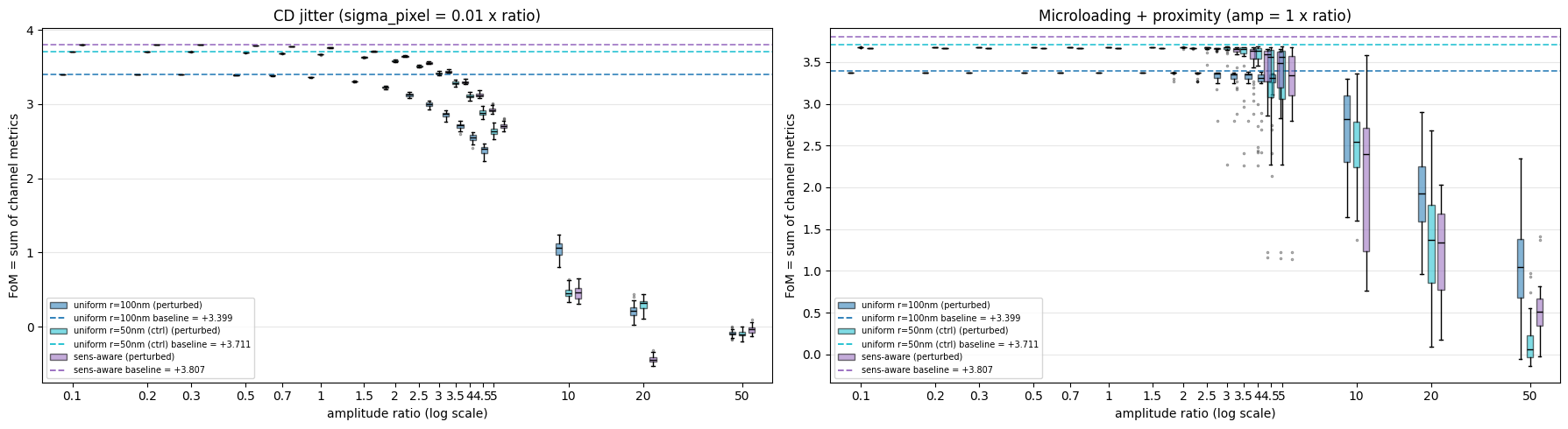
Analysis. For small to moderate amplitudes (the left half of each panel), the sens-aware boxes sit consistently above the uniform boxes and have tighter IQRs — the sens-aware design wins on both mean and standard deviation. As the amplitude grows past the transition region, the picture flips: at the largest ratios (right side), the uniform boxes dominate. The crossover happens roughly around ratio = 3 in CD jitter and microloading. So the sens-aware design is more robust against the physically realistic fab errors and gives up performance only under perturbations large enough to be off-spec for any modern foundry.
We caveat this read in the next plots — the box-and-whisker FoM hides the shape of the spectral degradation. (See the per-amplitude transmission spectra below.)
This paragraph is superseded. The "Sharpening the robustness comparison" section re-analyses exactly this data and shows that (a) the small-amplitude win is largely a baseline-offset artifact — under microloading it disappears entirely once each device is normalized by its own noise-free FoM — and (b) the genuine CD-jitter advantage is confined to ratios ≈1.5–5 and is worth ~2.5 pp of retention at most. Read that section before quoting the crossover.
One representative perturbed design per cell (seed = BASE_SEED, matching the leftmost MC sample of each box).
def viz_perturbations(perturb_fn, amplitudes, mc_label):
    devs = [(rho_uniform,   "uniform"),
            (rho_uniform50, "uniform-50nm"),
            (rho_sensaware, "sens-aware")]
    fig, axes = plt.subplots(len(devs), len(amplitudes),
                             figsize=(2.0 * len(amplitudes), 2.2 * len(devs)),
                             gridspec_kw=dict(wspace=0.05, hspace=0.10))
    for col, amp in enumerate(amplitudes):
        for row, (rho, dev_label) in enumerate(devs):
            rng      = np.random.default_rng(BASE_SEED)
            rho_pert = perturb_fn(np.asarray(rho, dtype=float), amp, rng)
            ax = axes[row, col]
            ax.imshow(np.flipud(1 - rho_pert.T), cmap="gray", vmin=0, vmax=1)
            ax.set_xticks([]); ax.set_yticks([])
            for spine in ax.spines.values():
                spine.set_visible(True); spine.set_color('0.4'); spine.set_linewidth(0.6)
            if row == 0:
                ax.set_title(f"r={RATIOS[col]:g}\namp={amp:g}", fontsize=8)
            if col == 0:
                ax.set_ylabel(dev_label, fontsize=11)
    fig.suptitle(f"{mc_label}: example perturbed designs at each amplitude (seed={BASE_SEED})",
                 fontsize=12, y=1.02)
    plt.show()

viz_perturbations(apply_cd_jitter,              CD_JITTER_AMPLITUDES,    "CD jitter")
viz_perturbations(apply_microloading_proximity, MICROLOADING_AMPLITUDES, "Microloading + proximity")
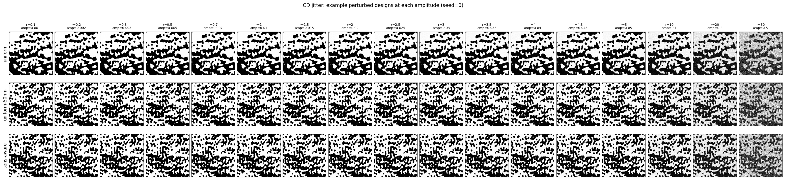
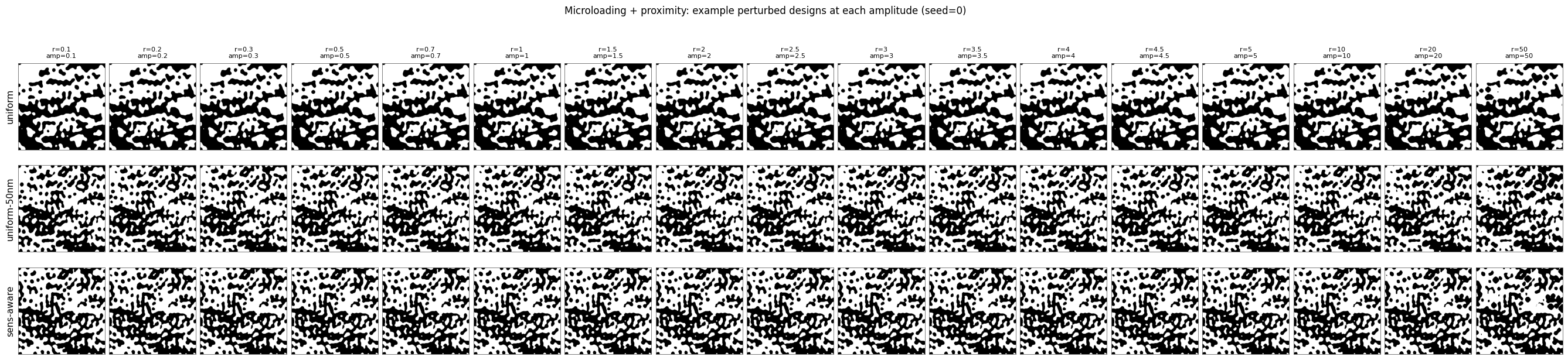
Mean transmission spectra across the 30 MC seeds per cell (151-point fine grid). Solid = mean across seeds, error bars = ±1 standard deviation across seeds at each wavelength. Dashed = noise-free reference. Error bars are subsampled (every 5th point) so the bands don't visually drown out the curves.
mc_freqs = np.array(mc_spec["freqs"])
mc_wvls  = 1000 * td.C_0 / mc_freqs
mc_cells = mc_spec["cells"]
mc_order = np.argsort(mc_wvls)
mc_wvls_sorted = mc_wvls[mc_order]

# per-row: (dev key used in the cell-dict keys, label, spectra-cells dict, noise-free ref)
_spec_rows = [
    ("uniform",   "uniform",      mc_cells,             ref_T_full["uniform"]),
    ("uniform50", "uniform-50nm", mc_spec_u50["cells"], ref_T_u50),
    ("sensaware", "sens-aware",   mc_cells,             ref_T_full["sensaware"]),
]

def plot_mc_spectra(mc_type, amplitudes, mc_label):
    fig, axes = plt.subplots(len(_spec_rows), len(amplitudes),
                             figsize=(2.2 * len(amplitudes), 2.7 * len(_spec_rows)),
                             sharex=True, sharey=True)
    for col, amp in enumerate(amplitudes):
        for row, (dev, dev_label, cells_src, ref) in enumerate(_spec_rows):
            ax = axes[row, col]
            for i in range(num_freqs_design):
                fmin, fmax = channel_bounds[i]
                ax.axvspan(1000 * td.C_0 / fmin, 1000 * td.C_0 / fmax,
                           alpha=0.12, color=colors[i])
            for i in range(num_freqs_design):
                ax.plot(mc_wvls_sorted, 100 * ref[i][mc_order],
                        color=colors[i], lw=0.8, ls="--", alpha=0.7)
            key = f"{mc_type}|{dev}|{amp:g}"
            mean_T = np.array(cells_src[key]["mean_T"])
            std_T  = np.array(cells_src[key]["std_T"])
            for i in range(num_freqs_design):
                ax.errorbar(mc_wvls_sorted,
                            100 * mean_T[i][mc_order],
                            yerr=100 * std_T[i][mc_order],
                            color=colors[i], lw=1.4,
                            ecolor=colors[i], elinewidth=0.6, capsize=1.5,
                            errorevery=5, alpha=0.95)
            ax.set_ylim(0, 100)
            ax.grid(alpha=0.3)
            if row == 0:
                ax.set_title(f"r={RATIOS[col]:g}", fontsize=9)
            if col == 0:
                ax.set_ylabel(f"{dev_label}\ntransmission (%)", fontsize=10)
            if row == len(_spec_rows) - 1:
                ax.set_xlabel("wavelength (nm)", fontsize=8)
    handles = [plt.Line2D([0], [0], color=colors[i], lw=1.6, label=f"port {i}")
               for i in range(num_freqs_design)]
    handles.append(plt.Line2D([0], [0], color="black", lw=0.8, ls="--",
                              label="noise-free reference"))
    fig.legend(handles=handles, loc="upper right", fontsize=9, ncol=5,
               bbox_to_anchor=(0.99, 1.02), frameon=True)
    fig.suptitle(f"{mc_label}: per-port mean +/- 1sigma across 30 MC seeds",
                 fontsize=12, y=1.04)
    plt.tight_layout()
    plt.show()

plot_mc_spectra("cdjitter",     CD_JITTER_AMPLITUDES,    "CD jitter")
plot_mc_spectra("microloading", MICROLOADING_AMPLITUDES, "Microloading + proximity")
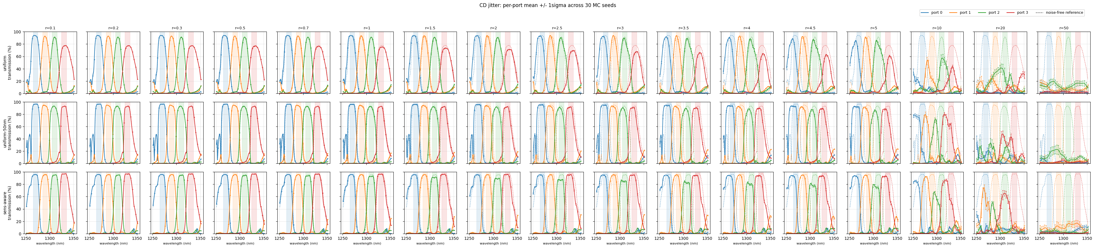
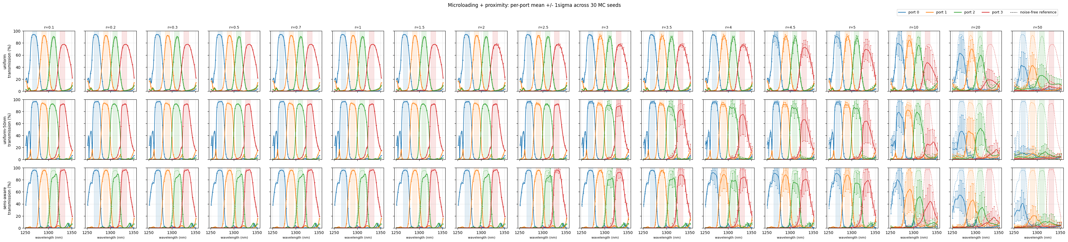
Analysis — caveat on the large-amplitude "uniform wins" region. Looking at the actual spectral shape, the two devices fail in qualitatively different ways under large fab error. For the uniform device, the dominant failure mode is a drop in peak transmission — the in-band peak gets shorter, with only a small wavelength shift. For the sens-aware device, the dominant failure mode is a wavelength shift of the peak — the peak height stays close to nominal, but the maximum moves outside the design band.
Because our channel-band-averaged FoM rewards transmission only inside the original design band, a peak that shifts out of band incurs a large FoM penalty even when the device is still doing demultiplexing — just at slightly different center wavelengths. Recentering the channel bands on the perturbed peaks would substantially recover the sens-aware FoM at large amplitudes; the uniform device's lost peak height is unrecoverable that way. So the "uniform wins at large amplitudes" reading from the box plots above is, at minimum, metric-dependent: against a wavelength-recentered FoM, the sens-aware win-rate would extend further to the right.
Uniform erosion-dilation
We sweep 11 amounts $\Delta \in \{-10, -8, -6, -4, -2, 0, +2, +4, +6, +8, +10\}\;\mathrm{nm}$ on each device — 22 simulations total, no random seeds. At $\Delta = 0$ the perturbation function returns the converged design unchanged (no SDF-tanh re-rasterization), so the $\Delta = 0$ point sits exactly on the noise-free eval baseline.
Sub-pixel resolution. The design grid is 15 nm pixels, but most of these amounts are sub-pixel. To capture sub-pixel boundary shifts we compute the binary mask's signed-distance field (in pixels), shift the zero-level set by $\Delta$, and pass the smooth-thresholded density to CustomMedium. The FDTD grid is much finer than 15 nm, so the simulator picks up the shift even though the design grid is coarser than the perturbation.
def apply_uniform_erosion_dilation(rho_clean, amount_nm, dl_um=dl_design_region):
    """Sub-pixel-resolved uniform morphological erosion (-) or dilation (+).

    Builds a binary mask, computes its signed-distance field in pixel units,
    shifts the zero-level set by amount_nm, and returns a smooth-thresholded
    [0, 1] density. CustomMedium will pick up the sub-pixel boundary shift.

    Special case: amount_nm == 0 returns rho_clean unchanged so the Δ=0 panel
    is the literal noise-free design (no SDF-tanh re-rasterization residual).
    """
    if amount_nm == 0:
        return rho_clean.copy()
    binary   = (rho_clean > 0.5)
    dist_in  = ndimage.distance_transform_edt( binary)
    dist_out = ndimage.distance_transform_edt(~binary)
    sdf_px   = dist_in - dist_out                              # +ve in solid
    amount_px = (amount_nm * 1e-3) / dl_um                     # nm -> um -> px
    return 0.5 * (1.0 + np.tanh(2.0 * (sdf_px + amount_px)))


# === ED sweep config: 11 amounts spanning ±10 nm ===
ED_AMOUNTS_NM = [-10, -8, -6, -4, -2, 0, 2, 4, 6, 8, 10]

CACHE_ED_U    = RESULTS_DIR / "mc_ed_uniform.json"
CACHE_ED_S    = RESULTS_DIR / "mc_ed_sensaware.json"
CACHE_ED_SPEC = RESULTS_DIR / "mc_ed_spectra.json"

if all(p.exists() for p in [CACHE_ED_U, CACHE_ED_S, CACHE_ED_SPEC]):
    ed_u    = json.loads(CACHE_ED_U.read_text())
    ed_s    = json.loads(CACHE_ED_S.read_text())
    ed_spec = json.loads(CACHE_ED_SPEC.read_text())
    print(f"loaded ED caches: {len(ed_u)} per device, {len(ed_spec['cells'])} spectra")
else:
    check_budget(2 * len(ED_AMOUNTS_NM), "ED sweep (uniform + sens-aware)", "perturbed", tag="ed")
    print("ED caches missing — building 22 sims (11 amounts × 2 devices) and dispatching")
    _ed_sim_data_dir = SIMDATA_DIR / "ed_dispatch"; _ed_sim_data_dir.mkdir(exist_ok=True)
    _ed_sims = {}
    _ed_index = {}
    for _rho, _dev in [(rho_uniform, "uniform"), (rho_sensaware, "sensaware")]:
        for _amt in ED_AMOUNTS_NM:
            _rho_p = apply_uniform_erosion_dilation(np.asarray(_rho, dtype=float), _amt)
            _task = f"hack_ed_{_dev}_amt{_amt:+g}nm"
            _ed_sims[_task]  = _build_perturbed_sim(_rho_p, fine_freqs=freqs_measure)
            _ed_index[_task] = (_dev, _amt)
    with quiet_tidy3d():
        _ed_batch = web.run_async(_ed_sims, path_dir=str(_ed_sim_data_dir), verbose=True)

    ed_u = {}; ed_s = {}
    _ed_spec_cells = {}
    _ed_freqs_master = None
    for _task, (_dev, _amt) in _ed_index.items():
        _sd = _ed_batch[_task]
        _chs = [float(get_metric(_sd, mnt_index=_i, leak_weight=1.0)) for _i in range(num_freqs_design)]
        _ports = []
        for _i in range(num_freqs_design):
            _a = _sd[f"mode_{_i}"].amps.sel(direction="+", mode_index=0)
            if _ed_freqs_master is None:
                _ed_freqs_master = np.array(_a.coords["f"]).tolist()
            _ports.append((np.abs(np.array(_a))**2).tolist())
        _rec = dict(amount_nm=_amt, channel_metrics=_chs)
        (ed_u if _dev == "uniform" else ed_s)[f"{_amt:+g}"] = _rec
        _ed_spec_cells[f"{_dev}|{_amt:+g}"] = dict(T=_ports)
    ed_spec = dict(freqs=_ed_freqs_master, cells=_ed_spec_cells)

    CACHE_ED_U.write_text(json.dumps(ed_u, indent=2))
    CACHE_ED_S.write_text(json.dumps(ed_s, indent=2))
    CACHE_ED_SPEC.write_text(json.dumps(ed_spec))
    print(f"saved ED caches: {len(ed_u)} per device, {len(ed_spec['cells'])} spectra")
loaded ED caches: 21 per device, 42 spectra
(g) Sum-FoM vs erosion-dilation amount. Single-line trace per device — no whisker because there is no random seed. Dashed horizontals are the noise-free baselines. $\Delta = 0$ short-circuits the SDF-tanh re-rasterization so it sits exactly on the baseline.
# (g) Sum-FoM vs erosion-dilation amount, now for ALL FOUR devices. The r=50nm
# control (uniform50, "50nm static") and the sens-aware online device both have
# cached ED sweeps, so these are read from disk -- no simulations. uniform50's
# baseline was computed with the primary MC figures above; the online baseline
# is computed here from its cached noise-free spectrum. `_tag` (online cache tag)
# is set in the online-filter configuration cell.
ed_u50 = json.loads((RESULTS_DIR / "mc_ed_uniform50_u50.json").read_text())
ed_o   = json.loads((RESULTS_DIR / f"mc_ed_online_{_tag}.json").read_text())
ref_T_online = np.array(json.loads((RESULTS_DIR / f"wdm_online_{_tag}_spectrum.json").read_text())["powers"])
baseline_o = baseline_sum_from_spectrum(ref_T_online, ref_freqs)


def _ed_sums(ed):
    return [sum(ed[f"{a:+g}"]["channel_metrics"]) for a in ED_AMOUNTS_NM]

sums_u   = _ed_sums(ed_u)      # kept (downstream cells reference sums_u / sums_s)
sums_u50 = _ed_sums(ed_u50)
sums_s   = _ed_sums(ed_s)
sums_o   = _ed_sums(ed_o)

_ed_series = [("uniform",   sums_u,   baseline_u),
              ("uniform50", sums_u50, baseline_u50),
              ("sensaware", sums_s,   baseline_s),
              ("online",    sums_o,   baseline_o)]

fig, ax = plt.subplots(figsize=(9.5, 5.2))
for key, sums, base in _ed_series:
    ax.plot(ED_AMOUNTS_NM, sums, "o-", color=DEV_COLORS[key], lw=1.6, ms=6,
            label=DEV_LABELS[key])
    ax.axhline(base, color=DEV_COLORS[key], ls="--", lw=1.2, alpha=0.7)
ax.axvline(0, color="black", lw=0.5, alpha=0.3)
ax.set_xlabel(r"$\Delta$  (nm)")
ax.set_ylabel("FoM = sum of channel metrics")
ax.set_title("Robustness to uniform erosion-dilation")
ax.set_xticks(ED_AMOUNTS_NM)
ax.grid(alpha=0.3)
ax.legend(fontsize=8, loc="lower center")
plt.tight_layout()
plt.show()
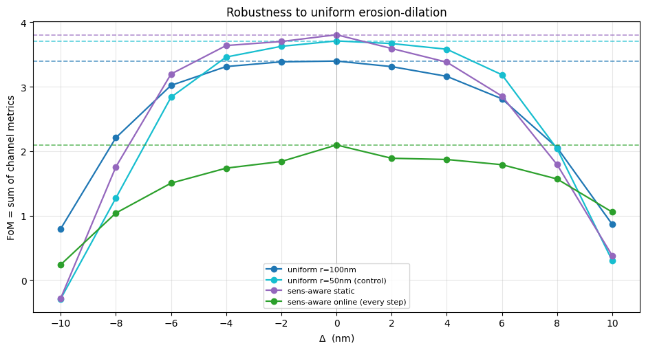
(h) Perturbed designs at each amount. Same SDF-tanh perturbation that was sent to the simulator. Solid = silicon, white = air.
fig, axes = plt.subplots(2, len(ED_AMOUNTS_NM),
                         figsize=(2.2 * len(ED_AMOUNTS_NM), 4.6),
                         gridspec_kw=dict(wspace=0.05, hspace=0.10))
for col, amt in enumerate(ED_AMOUNTS_NM):
    for row, (rho, dev_label) in enumerate(
            [(rho_uniform, "uniform"), (rho_sensaware, "sens-aware")]):
        rho_pert = apply_uniform_erosion_dilation(
            np.asarray(rho, dtype=float), amt, dl_um=dl_design_region)
        ax = axes[row, col]
        ax.imshow(np.flipud(1 - rho_pert.T), cmap="gray", vmin=0, vmax=1)
        ax.set_xticks([]); ax.set_yticks([])
        for spine in ax.spines.values():
            spine.set_visible(True); spine.set_color('0.4'); spine.set_linewidth(0.6)
        if row == 0:
            ax.set_title(f"{amt:+g} nm", fontsize=9)
        if col == 0:
            ax.set_ylabel(dev_label, fontsize=11)
fig.suptitle("Uniform erosion-dilation: perturbed designs at each amount",
             fontsize=12, y=1.02)
plt.show()
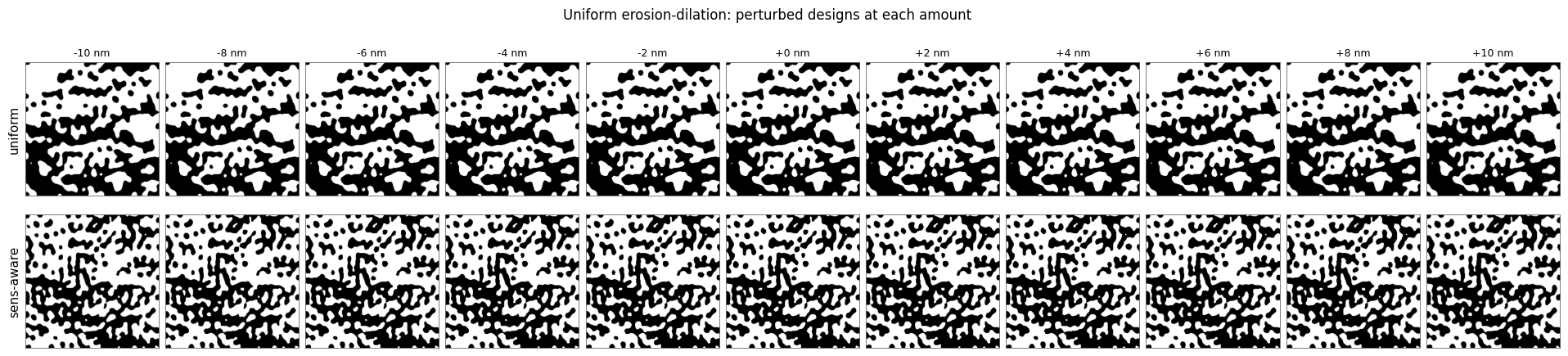
(i) Per-port transmission spectra at each amount. One sim per cell — no averaging required. Solid = perturbed, dashed = noise-free reference (151 fine-grid freqs).
ed_freqs   = np.array(ed_spec["freqs"])
ed_wvls_nm = 1000 * td.C_0 / ed_freqs
ed_cells   = ed_spec["cells"]
order = np.argsort(ed_wvls_nm)
ed_wvls_sorted = ed_wvls_nm[order]

fig, axes = plt.subplots(2, len(ED_AMOUNTS_NM), figsize=(2.5 * len(ED_AMOUNTS_NM), 5.6),
                         sharex=True, sharey=True)
for col, amt in enumerate(ED_AMOUNTS_NM):
    for row, dev in enumerate(["uniform", "sensaware"]):
        ax = axes[row, col]
        for i in range(num_freqs_design):
            fmin, fmax = channel_bounds[i]
            ax.axvspan(1000 * td.C_0 / fmin, 1000 * td.C_0 / fmax,
                       alpha=0.12, color=colors[i])
        ref = ref_T_full[dev]
        for i in range(num_freqs_design):
            ax.plot(ed_wvls_sorted, 100 * ref[i][order],
                    color=colors[i], lw=0.8, ls="--", alpha=0.7)
        T = np.array(ed_cells[f"{dev}|{amt:+g}"]["T"])
        for i in range(num_freqs_design):
            ax.plot(ed_wvls_sorted, 100 * T[i][order],
                    color=colors[i], lw=1.4)
        ax.set_ylim(0, 100)
        ax.grid(alpha=0.3)
        if row == 0:
            ax.set_title(f"{amt:+g} nm", fontsize=9)
        if col == 0:
            ax.set_ylabel(f"{dev}\ntransmission (%)", fontsize=10)
        if row == 1:
            ax.set_xlabel("wavelength (nm)", fontsize=8)
handles = [plt.Line2D([0], [0], color=colors[i], lw=1.6, label=f"port {i}")
           for i in range(num_freqs_design)]
handles.append(plt.Line2D([0], [0], color="black", lw=0.8, ls="--",
                          label="noise-free reference"))
fig.legend(handles=handles, loc="upper right", fontsize=9, ncol=5,
           bbox_to_anchor=(0.99, 1.02), frameon=True)
fig.suptitle("Uniform erosion-dilation: per-port transmission spectra (151 freqs)",
             fontsize=12, y=1.04)
plt.tight_layout()
plt.show()
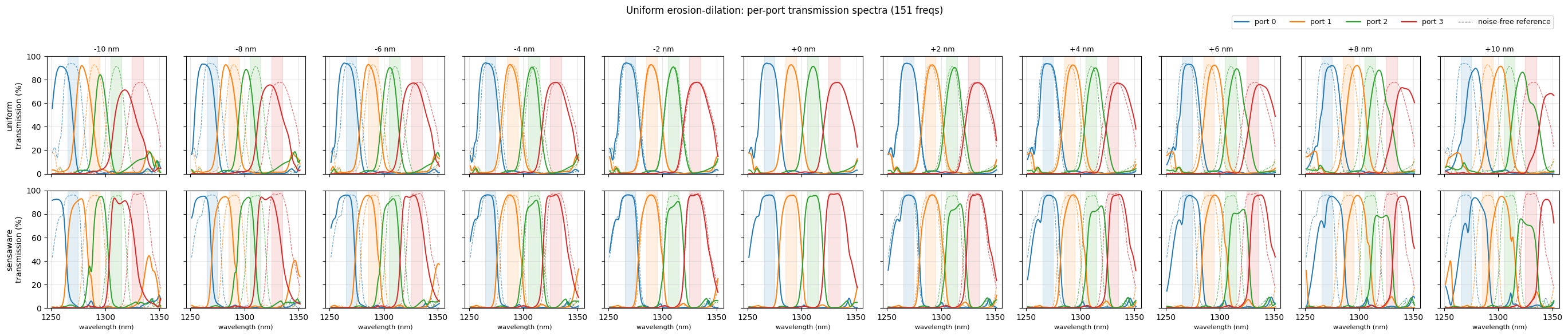
Robustness of the control and online devices
The same three noise models applied to the two devices added after the original study — the $r = 50$ nm control and the online-filter design — plotted alongside the two already characterized. Each new device writes its own cache files; nothing in the existing caches is touched.
Cost warning. A cold run of this section dispatches 1020 MC sims (17 amplitudes × 30 seeds × 2 noise models) plus 11 ED sims per new device — so ~2062 sims for both, roughly tripling the project's total cloud usage. The cells below are cache-or-dispatch like every other expensive cell, so they are free on a warm cache. To characterize only one of the two, trim EXTRA_DEVS.
# Devices added after the original two-way study. Each gets its own cache tag.
EXTRA_DEVS = [('uniform50', rho_uniform50, 'u50'),
              ('online',    rho_online,    _tag)]
if _SCHED_FULL:
    EXTRA_DEVS.append(('sched', rho_sched, _sched_tag))

# Devices permitted to dispatch a *fresh* sweep. Cached sweeps always load regardless;
# a device absent from this set with no cache simply skips. This is deliberately
# separate from ALLOW_DISPATCH: it stops one device's missing cache from quietly
# dragging a 1020-sim sweep along with another's.
FRESH_SWEEP_DEVS = {"sched"}
print(f"extra devices: {[d for d,_,_ in EXTRA_DEVS]}   fresh sweeps permitted for: {FRESH_SWEEP_DEVS}")

for _dev, _, _ in EXTRA_DEVS:
    ref_T_full[_dev] = np.array(SPECS[_dev]['powers'])

BASELINES = {'uniform': baseline_u, 'sensaware': baseline_s}
for _dev, _, _ in EXTRA_DEVS:
    BASELINES[_dev] = baseline_sum_from_spectrum(ref_T_full[_dev], ref_freqs)
if 'sched' in COMPARE_DEVS:          # spectrum only, no MC/ED sweeps for this device
    ref_T_full['sched'] = np.array(SPECS['sched']['powers'])
    BASELINES['sched'] = baseline_sum_from_spectrum(ref_T_full['sched'], ref_freqs)
baseline_o = BASELINES['online']          # kept for downstream references

print("noise-free baselines (151-freq metric):")
for _dev in COMPARE_DEVS:
    print(f"  {DEV_LABELS[_dev]:<28}{BASELINES[_dev]:+.4f}")
extra devices: ['uniform50', 'online', 'sched']   fresh sweeps permitted for: {'sched'}
noise-free baselines (151-freq metric):
  uniform r=100nm             +3.3987
  uniform r=50nm (control)    +3.7109
  sens-aware static           +3.8068
  sens-aware online (every step)+2.0961
  sens-aware online (every 10, frozen last 20)+2.8076
# === MC sweep for each extra device (cache-or-dispatch, own cache files per device) ===
import time
from collections import defaultdict

# Defined locally: the original two-way MC cell only binds these on its cache-miss
# path, so they are absent whenever those caches are warm.
CHUNK_SIZE, SLEEP_BETWEEN = 500, 30

MC_EXTRA = {}      # dev -> dict(cd=..., ml=..., spec=...)

def _run_mc_for_device(dev, rho_dev, tag):
    """Cache-or-dispatch the full CD-jitter + microloading sweep for one device."""
    c_cd   = RESULTS_DIR / f"mc_cdjitter_{dev}_{tag}.json"
    c_ml   = RESULTS_DIR / f"mc_microloading_{dev}_{tag}.json"
    c_spec = RESULTS_DIR / f"mc_spectra_{dev}_{tag}.json"

    if all(p.exists() for p in (c_cd, c_ml, c_spec)):
        out = dict(cd=json.loads(c_cd.read_text()), ml=json.loads(c_ml.read_text()),
                   spec=json.loads(c_spec.read_text()))
        print(f"[{dev}] loaded MC caches: {len(out['cd'])} CD amps, "
              f"{len(out['ml'])} ML amps, {len(out['spec']['cells'])} mean spectra")
        return out

    if dev not in FRESH_SWEEP_DEVS:
        print(f"[{dev}] MC caches missing but '{dev}' is not in FRESH_SWEEP_DEVS -> SKIPPING "
              f"({len(RATIOS)*N_SAMPLES*2} sims not submitted).")
        return None
    if not dispatch_allowed("mc"):
        print(f"[{dev}] MC caches missing and 'mc' dispatch is not permitted -> SKIPPING "
              f"({len(RATIOS)*N_SAMPLES*2} sims not submitted). This device is omitted "
              f"from the MC figures below.")
        return None
    check_budget(len(RATIOS) * N_SAMPLES * 2, f"MC sweep [{dev}]", "perturbed", tag="mc")
    print(f"[{dev}] MC caches missing — dispatching {len(RATIOS)*N_SAMPLES*2} sims "
          f"({len(RATIOS)} amps x {N_SAMPLES} seeds x 2 noise models)")
    mc_cd, mc_ml = {}, {}
    spec_accum = defaultdict(list)
    freqs_master = None
    out_dir = SIMDATA_DIR / f"mc_{dev}_{tag}"; out_dir.mkdir(exist_ok=True)

    def robust_run(sims, label, max_retries=5):
        delay = 60
        for attempt in range(1, max_retries + 1):
            try:
                return web.run_async(sims, path_dir=str(out_dir), verbose=True)
            except Exception as e:
                print(f"[{label}] attempt {attempt} failed: {str(e)[:150]}")
                if attempt == max_retries:
                    raise
                print(f"[{label}] sleeping {delay}s before retry...")
                time.sleep(delay)
                delay = min(delay * 2, 600)

    def dispatch(perturb_fn, mc_label, amplitudes, cache):
        nonlocal freqs_master
        sims, idx = {}, {}
        rho_np = np.asarray(rho_dev, dtype=float)
        for amp in amplitudes:
            for seed in range(BASE_SEED, BASE_SEED + N_SAMPLES):
                rng = np.random.default_rng(seed)
                task = f"hack_{mc_label}_{dev}_{tag}_amp{amp:g}_seed{seed}"
                sims[task] = _build_perturbed_sim(perturb_fn(rho_np, amp, rng),
                                                  fine_freqs=freqs_measure)
                idx[task]  = (amp, seed)
        items = list(sims.items())
        n_chunks = (len(items) + CHUNK_SIZE - 1) // CHUNK_SIZE
        print(f"=== {dev} {mc_label}: {len(items)} sims -> {n_chunks} chunk(s) ===")
        for ci in range(n_chunks):
            chunk = dict(items[ci*CHUNK_SIZE:(ci+1)*CHUNK_SIZE])
            print(f"--- {dev} {mc_label} chunk {ci+1}/{n_chunks} ({len(chunk)} sims) ---")
            bd = robust_run(chunk, f"{dev}-{mc_label}-chunk{ci+1}")
            for task in chunk:
                sd = bd[task]
                amp, seed = idx[task]
                chs = [float(get_metric(sd, mnt_index=i, leak_weight=1.0))
                       for i in range(num_freqs_design)]
                ports = []
                for i in range(num_freqs_design):
                    a = sd[f"mode_{i}"].amps.sel(direction="+", mode_index=0)
                    if freqs_master is None:
                        freqs_master = np.array(a.coords["f"]).tolist()
                    ports.append((np.abs(np.array(a))**2).tolist())
                cache.setdefault(f"{amp:g}", []).append(
                    dict(seed=int(seed), channel_metrics=chs))
                spec_accum[(mc_label, f"{amp:g}")].append(np.array(ports))
            del bd
            if ci + 1 < n_chunks:
                print(f"--- sleeping {SLEEP_BETWEEN}s before next chunk ---")
                time.sleep(SLEEP_BETWEEN)

    with quiet_tidy3d():
        dispatch(apply_cd_jitter, "cdjitter", CD_JITTER_AMPLITUDES, mc_cd)
        print(f"--- sleeping {SLEEP_BETWEEN}s between MC types ---")
        time.sleep(SLEEP_BETWEEN)
        dispatch(apply_microloading_proximity, "microloading",
                 MICROLOADING_AMPLITUDES, mc_ml)

    spec = dict(freqs=freqs_master, cells={})
    for (mc_type, amp_key), arrs in spec_accum.items():
        arr = np.stack(arrs, axis=0)
        spec["cells"][f"{mc_type}|{dev}|{amp_key}"] = dict(
            mean_T=arr.mean(axis=0).tolist(), std_T=arr.std(axis=0).tolist(),
            n_seeds=arr.shape[0])

    c_cd.write_text(json.dumps(mc_cd, indent=2))
    c_ml.write_text(json.dumps(mc_ml, indent=2))
    c_spec.write_text(json.dumps(spec))
    print(f"[{dev}] saved MC caches: {len(mc_cd)} CD amps, {len(mc_ml)} ML amps")
    return dict(cd=mc_cd, ml=mc_ml, spec=spec)


for _dev, _rho, _tag in EXTRA_DEVS:
    _res = _run_mc_for_device(_dev, _rho, _tag)
    if _res is not None:
        MC_EXTRA[_dev] = _res

print()
print(f"devices with MC data: {['uniform', 'sensaware'] + list(MC_EXTRA)}")

# Back-compat aliases (only if the online device actually has MC data).
if 'online' in MC_EXTRA:
    mc_cd_o, mc_ml_o, mc_spec_o = (MC_EXTRA['online']['cd'], MC_EXTRA['online']['ml'],
                                   MC_EXTRA['online']['spec'])
[uniform50] loaded MC caches: 17 CD amps, 17 ML amps, 34 mean spectra
[online] MC caches missing but 'online' is not in FRESH_SWEEP_DEVS -> SKIPPING (1020 sims not submitted).
[sched] loaded MC caches: 17 CD amps, 17 ML amps, 34 mean spectra

devices with MC data: ['uniform', 'sensaware', 'uniform50', 'sched']
Four-way box plots. Same $\sum_i m_i$ FoM, 30 seeds per cell, dashed horizontals at each device's own noise-free baseline. Note these are absolute FoM — see "Sharpening the robustness comparison" below for the normalized version, which is the one to trust when the baselines differ.
CD_SUMS = {'uniform': cd_u_sums, 'sensaware': cd_s_sums}
ML_SUMS = {'uniform': ml_u_sums, 'sensaware': ml_s_sums}
for _dev in MC_EXTRA:
    CD_SUMS[_dev] = extract_sums(MC_EXTRA[_dev]['cd'], CD_JITTER_AMPLITUDES)
    ML_SUMS[_dev] = extract_sums(MC_EXTRA[_dev]['ml'], MICROLOADING_AMPLITUDES)
if 'online' in CD_SUMS:
    cd_o_sums, ml_o_sums = CD_SUMS['online'], ML_SUMS['online']

def whisker_group(ax, datasets, ratios, title, xlabel):
    """datasets: list of (device_key, list-of-sample-lists), one box per device per ratio."""
    r = np.asarray(ratios, dtype=float)
    n_dev = len(datasets)
    spread = 0.10
    offsets = np.linspace(-spread, spread, n_dev)
    for (dev_key, data), off in zip(datasets, offsets):
        pos = r * np.exp(off)
        width = pos * (np.exp(spread) - np.exp(-spread)) * 0.45 / max(n_dev - 1, 1)
        bp = ax.boxplot(data, positions=pos, widths=width, patch_artist=True)
        for box in bp["boxes"]:
            box.set_facecolor(DEV_COLORS[dev_key]); box.set_alpha(0.55)
            box.set_edgecolor("black")
        for elem in ("whiskers", "caps", "medians"):
            for line in bp[elem]:
                line.set_color("black")
        for flier in bp["fliers"]:
            flier.set(marker=".", markersize=3, alpha=0.4)
        ax.axhline(BASELINES[dev_key], color=DEV_COLORS[dev_key], ls="--", lw=1.2, alpha=0.85)
    ax.set_xscale("log")
    ax.set_xticks(r); ax.set_xticklabels([f"{x:g}" for x in r])
    ax.tick_params(axis="x", which="minor", bottom=False)
    ax.set_xlim(r.min() / np.exp(3*spread), r.max() * np.exp(3*spread))
    ax.set_xlabel(xlabel); ax.set_ylabel("FoM = sum of channel metrics")
    ax.set_title(title); ax.grid(alpha=0.3, axis="y")
    ax.legend([Patch(facecolor=DEV_COLORS[k], alpha=0.55, edgecolor="black")
               for k, _ in datasets]
              + [Line2D([0], [0], color=DEV_COLORS[k], ls="--", lw=1.2) for k, _ in datasets],
              [DEV_LABELS[k] for k, _ in datasets]
              + [f"{DEV_LABELS[k]} baseline = {BASELINES[k]:+.3f}" for k, _ in datasets],
              loc="lower left", fontsize=7, ncol=2)

_BOX_DEVS = [d for d in COMPARE_DEVS if d in CD_SUMS]

fig, axes = plt.subplots(1, 2, figsize=(20, 5.8))
whisker_group(axes[0], [(d, CD_SUMS[d]) for d in _BOX_DEVS],
              RATIOS, f"CD jitter (sigma_pixel = {CD_JITTER_BASE} × ratio)",
              "amplitude ratio (log scale)")
whisker_group(axes[1], [(d, ML_SUMS[d]) for d in _BOX_DEVS],
              RATIOS, f"Microloading + proximity (amp = {MICROLOADING_BASE:g} × ratio)",
              "amplitude ratio (log scale)")
plt.tight_layout()
plt.show()

# Numeric win/loss table: mean +- std of the FoM per amplitude, every device.
def _summ(sums):
    return np.array([np.mean(v) for v in sums]), np.array([np.std(v) for v in sums])

for _mc_name, _store in [("CD jitter", CD_SUMS), ("Microloading", ML_SUMS)]:
    _mu = {d: _summ(_store[d])[0] for d in _BOX_DEVS}
    _sd = {d: _summ(_store[d])[1] for d in _BOX_DEVS}
    print(f"\n{_mc_name} - mean +- std of sum-FoM across {N_SAMPLES} seeds")
    print(f"  {'ratio':>7}" + "".join(f"{DEV_LABELS[d]:>26}" for d in _BOX_DEVS) + "   best")
    for k, rr in enumerate(RATIOS):
        _best = max(_BOX_DEVS, key=lambda d: _mu[d][k])
        print(f"  {rr:>7g}"
              + "".join(f"{_mu[d][k]:>17.3f}+-{_sd[d][k]:<7.3f}" for d in _BOX_DEVS)
              + f"   {DEV_LABELS[_best]}")
    # the control comparison, on absolute FoM
    if 'uniform50' in _mu:
        for _cand in ('sensaware', 'online'):
            if _cand in _mu:
                print(f"  {DEV_LABELS[_cand]} beats the r=50nm control on mean at "
                      f"{100*np.mean(_mu[_cand] > _mu['uniform50']):.0f}% of amplitudes; "
                      f"on std at {100*np.mean(_sd[_cand] < _sd['uniform50']):.0f}%")
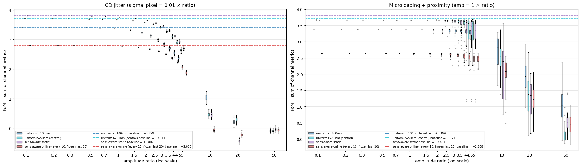
CD jitter - mean +- std of sum-FoM across 30 seeds
    ratio           uniform r=100nm  uniform r=50nm (control)         sens-aware staticsens-aware online (every 10, frozen last 20)   best
      0.1            3.400+-0.000              3.709+-0.000              3.805+-0.000              2.807+-0.000     sens-aware static
      0.2            3.400+-0.000              3.706+-0.000              3.803+-0.000              2.805+-0.000     sens-aware static
      0.3            3.399+-0.001              3.703+-0.000              3.800+-0.000              2.803+-0.000     sens-aware static
      0.5            3.394+-0.001              3.695+-0.001              3.792+-0.001              2.797+-0.000     sens-aware static
      0.7            3.384+-0.002              3.686+-0.001              3.781+-0.001              2.789+-0.001     sens-aware static
        1            3.363+-0.003              3.670+-0.002              3.761+-0.002              2.773+-0.001     sens-aware static
      1.5            3.307+-0.006              3.633+-0.003              3.713+-0.004              2.735+-0.003     sens-aware static
        2            3.226+-0.012              3.582+-0.006              3.645+-0.007              2.679+-0.005     sens-aware static
      2.5            3.122+-0.018              3.512+-0.010              3.555+-0.010              2.602+-0.009     sens-aware static
        3            2.998+-0.026              3.416+-0.015              3.440+-0.015              2.499+-0.013     sens-aware static
      3.5            2.857+-0.034              3.284+-0.023              3.296+-0.021              2.372+-0.020     sens-aware static
        4            2.704+-0.041              3.108+-0.033              3.124+-0.028              2.227+-0.027     sens-aware static
      4.5            2.543+-0.048              2.888+-0.044              2.926+-0.036              2.063+-0.034     sens-aware static
        5            2.379+-0.055              2.635+-0.054              2.708+-0.043              1.879+-0.042     sens-aware static
       10            1.036+-0.118              0.468+-0.074              0.460+-0.086             -0.057+-0.058     uniform r=100nm
       20            0.217+-0.094              0.301+-0.078             -0.440+-0.053             -0.217+-0.050     uniform r=50nm (control)
       50           -0.091+-0.041             -0.099+-0.044             -0.040+-0.055             -0.062+-0.043     sens-aware static
  sens-aware static beats the r=50nm control on mean at 88% of amplitudes; on std at 29%

Microloading - mean +- std of sum-FoM across 30 seeds
    ratio           uniform r=100nm  uniform r=50nm (control)         sens-aware staticsens-aware online (every 10, frozen last 20)   best
      0.1            3.371+-0.000              3.678+-0.000              3.665+-0.000              2.639+-0.000     uniform r=50nm (control)
      0.2            3.371+-0.000              3.678+-0.000              3.665+-0.000              2.639+-0.000     uniform r=50nm (control)
      0.3            3.371+-0.000              3.678+-0.000              3.665+-0.000              2.639+-0.000     uniform r=50nm (control)
      0.5            3.371+-0.000              3.678+-0.000              3.665+-0.000              2.639+-0.000     uniform r=50nm (control)
      0.7            3.371+-0.000              3.678+-0.000              3.665+-0.000              2.639+-0.000     uniform r=50nm (control)
        1            3.371+-0.000              3.678+-0.000              3.665+-0.000              2.638+-0.004     uniform r=50nm (control)
      1.5            3.371+-0.000              3.678+-0.000              3.665+-0.000              2.632+-0.019     uniform r=50nm (control)
        2            3.365+-0.022              3.678+-0.003              3.665+-0.001              2.622+-0.039     uniform r=50nm (control)
      2.5            3.355+-0.035              3.666+-0.039              3.644+-0.088              2.603+-0.053     uniform r=50nm (control)
        3            3.325+-0.105              3.613+-0.252              3.573+-0.187              2.586+-0.061     uniform r=50nm (control)
      3.5            3.318+-0.104              3.514+-0.356              3.526+-0.215              2.556+-0.081     sens-aware static
        4            3.313+-0.103              3.416+-0.446              3.332+-0.613              2.505+-0.122     uniform r=50nm (control)
      4.5            3.232+-0.222              3.322+-0.447              3.242+-0.609              2.484+-0.122     uniform r=50nm (control)
        5            3.189+-0.295              3.284+-0.460              3.186+-0.601              2.471+-0.129     uniform r=50nm (control)
       10            2.669+-0.487              2.500+-0.468              2.116+-0.842              2.008+-0.483     uniform r=100nm
       20            1.893+-0.467              1.351+-0.626              1.206+-0.595              1.232+-0.438     uniform r=100nm
       50            1.001+-0.559              0.170+-0.295              0.525+-0.315              0.438+-0.319     uniform r=100nm
  sens-aware static beats the r=50nm control on mean at 12% of amplitudes; on std at 65%
Four-way mean spectra across the 30 MC seeds, at a subset of amplitudes spanning the crossover region.
# device -> the mean-spectrum cell dict holding its data
MC_CELLS_FOR = {'uniform': mc_cells, 'sensaware': mc_cells}
for _dev in MC_EXTRA:
    MC_CELLS_FOR[_dev] = MC_EXTRA[_dev]['spec']['cells']

def plot_mc_spectra_3way(mc_type, amplitudes, mc_label, ratios):
    devs = [(d, MC_CELLS_FOR[d]) for d in COMPARE_DEVS if d in MC_CELLS_FOR]
    fig, axes = plt.subplots(len(devs), len(amplitudes),
                             figsize=(2.2 * len(amplitudes), 2.5 * len(devs)),
                             sharex=True, sharey=True, squeeze=False)
    for col, amp in enumerate(amplitudes):
        for row, (dev, cells) in enumerate(devs):
            ax = axes[row, col]
            for i in range(num_freqs_design):
                fmin, fmax = channel_bounds[i]
                ax.axvspan(1000 * td.C_0 / fmin, 1000 * td.C_0 / fmax,
                           alpha=0.12, color=colors[i])
            ref = ref_T_full[dev]
            for i in range(num_freqs_design):
                ax.plot(mc_wvls_sorted, 100 * ref[i][mc_order],
                        color=colors[i], lw=0.8, ls="--", alpha=0.7)
            key = f"{mc_type}|{dev}|{amp:g}"
            mean_T = np.array(cells[key]["mean_T"]); std_T = np.array(cells[key]["std_T"])
            for i in range(num_freqs_design):
                ax.errorbar(mc_wvls_sorted, 100 * mean_T[i][mc_order],
                            yerr=100 * std_T[i][mc_order], color=colors[i], lw=1.4,
                            ecolor=colors[i], elinewidth=0.6, capsize=1.5,
                            errorevery=5, alpha=0.95)
            ax.set_ylim(0, 100); ax.grid(alpha=0.3)
            if row == 0:
                ax.set_title(f"r={ratios[col]:g}", fontsize=9)
            if col == 0:
                ax.set_ylabel(f"{DEV_LABELS[dev]}\ntransmission (%)", fontsize=8)
            if row == len(devs) - 1:
                ax.set_xlabel("wavelength (nm)", fontsize=8)
    handles = [plt.Line2D([0], [0], color=colors[i], lw=1.6, label=f"port {i}")
               for i in range(num_freqs_design)]
    handles.append(plt.Line2D([0], [0], color="black", lw=0.8, ls="--",
                              label="noise-free reference"))
    fig.legend(handles=handles, loc="upper right", fontsize=9, ncol=5,
               bbox_to_anchor=(0.99, 1.02), frameon=True)
    fig.suptitle(f"{mc_label}: per-port mean ± 1σ across {N_SAMPLES} MC seeds — all devices",
                 fontsize=12, y=1.03)
    plt.tight_layout()
    plt.show()

# Subset of amplitudes around the crossover, to keep the grid readable.
# Falls back to every cached ratio if none of the preferred subset is present.
_sub_ratios = [r for r in RATIOS if r in (0.1, 0.5, 1, 2, 3, 5, 10, 50)] or list(RATIOS)
_sub_idx    = [RATIOS.index(r) for r in _sub_ratios]
plot_mc_spectra_3way("cdjitter", [CD_JITTER_AMPLITUDES[i] for i in _sub_idx],
                     "CD jitter", _sub_ratios)
plot_mc_spectra_3way("microloading", [MICROLOADING_AMPLITUDES[i] for i in _sub_idx],
                     "Microloading + proximity", _sub_ratios)
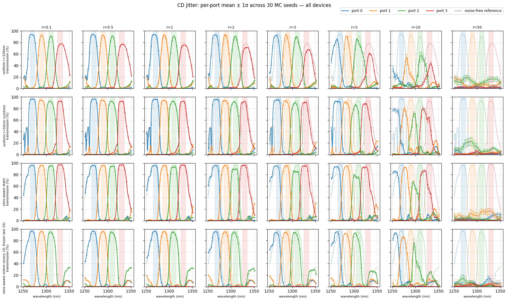
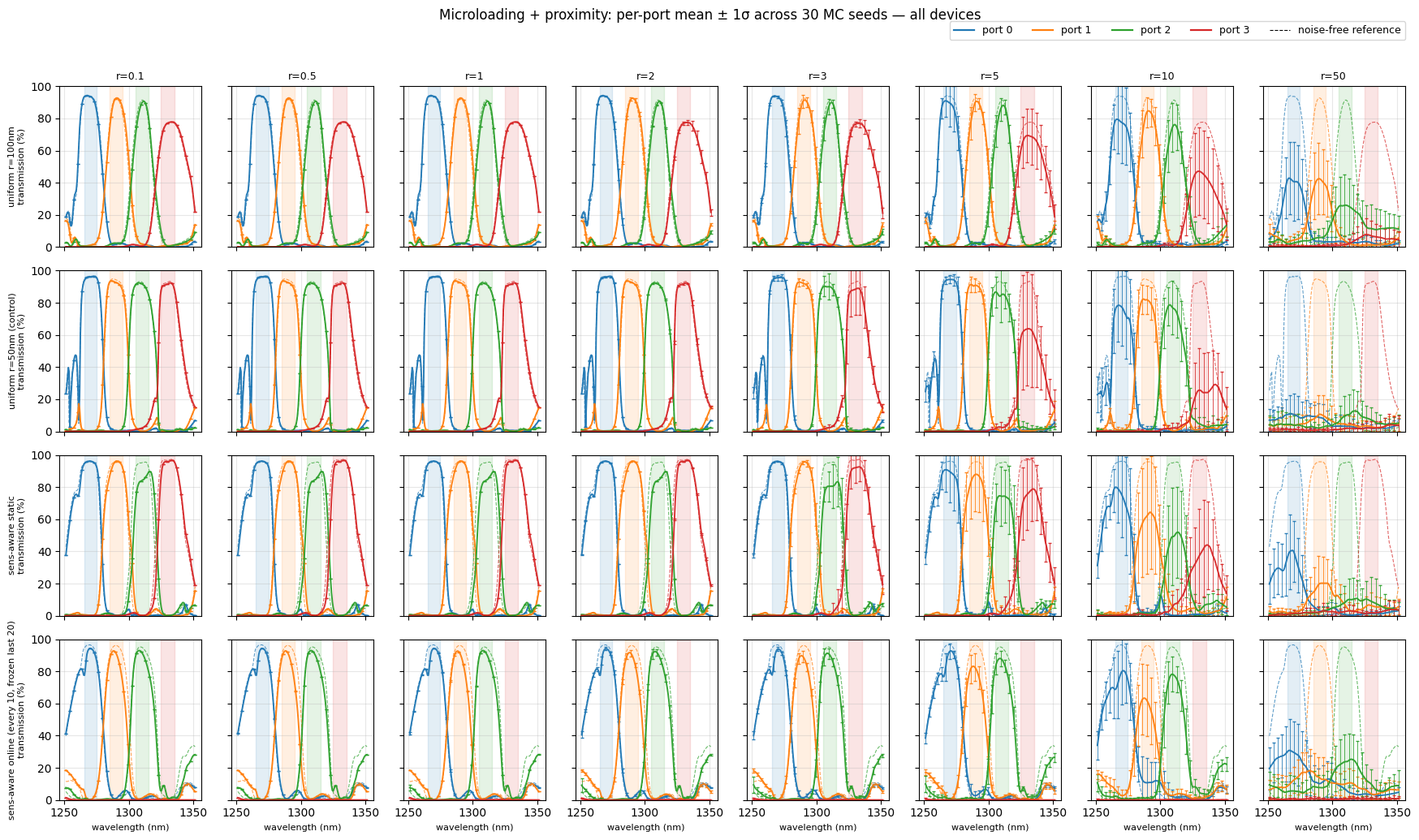
Three-way erosion-dilation. Deterministic sweep, 11 amounts, one sim per point.
def _run_ed_for_device(dev, rho_dev, tag):
    """Cache-or-dispatch the 11-point erosion-dilation sweep for one device."""
    c_ed   = RESULTS_DIR / f"mc_ed_{dev}_{tag}.json"
    c_spec = RESULTS_DIR / f"mc_ed_spectra_{dev}_{tag}.json"
    if c_ed.exists() and c_spec.exists():
        ed = json.loads(c_ed.read_text()); spec = json.loads(c_spec.read_text())
        print(f"[{dev}] loaded ED caches: {len(ed)} amounts")
        return ed, spec

    if dev not in FRESH_SWEEP_DEVS:
        print(f"[{dev}] ED caches missing but '{dev}' is not in FRESH_SWEEP_DEVS -> SKIPPING.")
        return None
    if not dispatch_allowed("ed"):
        print(f"[{dev}] ED caches missing and 'ed' dispatch is not permitted -> SKIPPING "
              f"({len(ED_AMOUNTS_NM)} sims not submitted). This device is omitted "
              f"from the ED figure below.")
        return None
    check_budget(len(ED_AMOUNTS_NM), f"ED sweep [{dev}]", "perturbed", tag="ed")
    print(f"[{dev}] ED caches missing - building {len(ED_AMOUNTS_NM)} sims and dispatching")
    out_dir = SIMDATA_DIR / f"ed_{dev}_{tag}"; out_dir.mkdir(exist_ok=True)
    sims, idx = {}, {}
    for amt in ED_AMOUNTS_NM:
        rho_p = apply_uniform_erosion_dilation(np.asarray(rho_dev, dtype=float), amt)
        task = f"hack_ed_{dev}_{tag}_amt{amt:+g}nm"
        sims[task] = _build_perturbed_sim(rho_p, fine_freqs=freqs_measure)
        idx[task]  = amt
    with quiet_tidy3d():
        bd = web.run_async(sims, path_dir=str(out_dir), verbose=True)

    ed, cells, freqs_master = {}, {}, None
    for task, amt in idx.items():
        sd = bd[task]
        chs = [float(get_metric(sd, mnt_index=i, leak_weight=1.0))
               for i in range(num_freqs_design)]
        ports = []
        for i in range(num_freqs_design):
            a = sd[f"mode_{i}"].amps.sel(direction="+", mode_index=0)
            if freqs_master is None:
                freqs_master = np.array(a.coords["f"]).tolist()
            ports.append((np.abs(np.array(a))**2).tolist())
        ed[f"{amt:+g}"] = dict(amount_nm=amt, channel_metrics=chs)
        cells[f"{dev}|{amt:+g}"] = dict(T=ports)
    spec = dict(freqs=freqs_master, cells=cells)
    c_ed.write_text(json.dumps(ed, indent=2))
    c_spec.write_text(json.dumps(spec))
    print(f"[{dev}] saved ED caches: {len(ed)} amounts")
    return ed, spec


ED_EXTRA = {}
for _dev, _rho, _tag in EXTRA_DEVS:
    _res = _run_ed_for_device(_dev, _rho, _tag)
    if _res is not None:
        ED_EXTRA[_dev] = _res
if 'online' in ED_EXTRA:
    ed_o, ed_spec_o = ED_EXTRA['online']    # back-compat aliases

ED_SUMS = {'uniform': sums_u, 'sensaware': sums_s}
for _dev in ED_EXTRA:
    ED_SUMS[_dev] = [sum(ED_EXTRA[_dev][0][f"{a:+g}"]["channel_metrics"])
                     for a in ED_AMOUNTS_NM]
if 'online' in ED_SUMS:
    sums_o = ED_SUMS['online']
_ED_DEVS = [d for d in COMPARE_DEVS if d in ED_SUMS]

fig, ax = plt.subplots(figsize=(9.5, 5.2))
for _key in _ED_DEVS:
    ax.plot(ED_AMOUNTS_NM, ED_SUMS[_key], "o-", color=DEV_COLORS[_key], lw=1.6, ms=6,
            label=DEV_LABELS[_key])
    ax.axhline(BASELINES[_key], color=DEV_COLORS[_key], ls="--", lw=1.2, alpha=0.85)
ax.axvline(0, color="black", lw=0.5, alpha=0.3)
ax.set_xlabel(r"$\Delta$  (nm)"); ax.set_ylabel("FoM = sum of channel metrics")
ax.set_title("Robustness to uniform erosion-dilation — all devices")
ax.set_xticks(ED_AMOUNTS_NM); ax.grid(alpha=0.3)
ax.legend(fontsize=8, loc="lower center")
plt.tight_layout()
plt.show()

print("ED FoM retention (perturbed / own baseline), mean over the +-10 nm sweep:")
for _key in _ED_DEVS:
    print(f"  {DEV_LABELS[_key]:<28} "
          f"{100*np.mean(np.array(ED_SUMS[_key])/BASELINES[_key]):.1f}%")
[uniform50] loaded ED caches: 11 amounts
[online] loaded ED caches: 11 amounts
[sched] loaded ED caches: 11 amounts
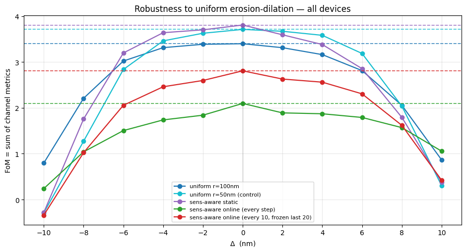
ED FoM retention (perturbed / own baseline), mean over the +-10 nm sweep:
  uniform r=100nm              75.8%
  uniform r=50nm (control)     67.1%
  sens-aware static            66.4%
  sens-aware online (every step) 72.1%
  sens-aware online (every 10, frozen last 20) 65.2%
Sharpening the robustness comparison
Everything in this section is post-processing on the caches already loaded above — no new simulations. It addresses three ways the box plots overstate (or understate) what the data supports.
- Absolute FoM confounds robustness with baseline. The devices do not start from the same noise-free FoM (uniform $+3.40$, sens-aware $+3.81$), so a device can look more robust simply by having had further to fall. Robustness is about degradation, so we normalize each device by its own baseline.
-
The box plots discard the pairing. For CD jitter the comparison is exactly paired:
np.random.default_rng(seed)produces the identical $300\times300$ noise field for both devices, so per-seed differences are meaningful and admit a much tighter confidence interval than the marginal spreads suggest. (Microloading is not paired — the two designs have different feature counts, sorng.normal(0, sigmas)draws vectors of different length and consumes the stream differently.) - The "shift vs. peak-drop" claim was qualitative. We can measure it: extract per-port peak wavelength and peak height, and recompute the FoM against channel bands shifted by a single global $\delta\lambda$ chosen to maximize it. That directly tests the Discussion's hypothesis that a wavelength-recentered metric would extend the sens-aware win.
Caveat on (3). Only the mean spectrum across the 30 seeds was cached, not per-seed spectra. Averaging spectra that have each shifted by a different random amount smears the peaks, which biases measured peak heights downward and shifts toward zero. So the recentering numbers below are a lower bound on what a per-seed analysis would show. Recovering per-seed spectra needs the raw MC hdf5s (archived, not shipped) or a re-dispatch.
# ---- shared re-analysis helpers (post-processing only) ----
def fom_shifted(P, F, shift=0.0):
    """Sum of per-channel metrics with every channel band shifted by `shift` (Hz).

    Reduces exactly to baseline_sum_from_spectrum() at shift = 0.
    """
    nb = num_freqs_design
    T = np.zeros((nb, nb))
    for port in range(nb):
        for band in range(nb):
            m = ((F >= channel_bounds[band][0] + shift) &
                 (F <= channel_bounds[band][1] + shift))
            T[port, band] = P[port, m].mean() if m.any() else 0.0
    return float(sum(T[i, i] - sum(T[i, j] for j in range(nb) if j != i) / (nb - 1)
                     for i in range(nb)))


def best_recentering(P, F, n_delta=161, span=0.7):
    """Global band shift maximizing the FoM. Returns (delta_Hz, FoM_best, FoM_at_zero)."""
    deltas = np.linspace(-span * df_design, span * df_design, n_delta)
    vals = [fom_shifted(P, F, d) for d in deltas]
    k = int(np.argmax(vals))
    return deltas[k], vals[k], fom_shifted(P, F, 0.0)


def port_peaks(P, F):
    """Per-port (peak wavelength nm, peak height) searched within ±1 channel spacing."""
    W = 1000 * td.C_0 / F
    out = []
    for i in range(num_freqs_design):
        m = np.abs(F - float(freqs_design[i])) <= df_design
        w, p = W[m], P[i][m]
        k = int(np.argmax(p))
        out.append((w[k], p[k]))
    return np.array(out)


def seed_sums(records, amp):
    """Per-seed sum-FoM for one amplitude, ordered by seed (so devices align)."""
    return np.array([sum(r["channel_metrics"])
                     for r in sorted(records[f"{amp:g}"], key=lambda z: z["seed"])])


# Fraction of the FoM lost to the perturbation that recentering wins back. Undefined
# when nothing was lost (e.g. the ED sweep's delta = 0 point sits on the baseline), so
# guard rather than divide by ~0.
MIN_LOSS = 1e-3

def recovered_frac(fom_best, fom_zero, baseline):
    loss = baseline - fom_zero
    return 100.0 * (fom_best - fom_zero) / loss if loss > MIN_LOSS else float('nan')

def fmt_recovered(x):
    return "     n/a" if not np.isfinite(x) else f"{x:>7.1f}%"


# Which devices have data loaded? The two originals always; the extras only if their
# sections ran. Detected from the data itself rather than a build-time flag, so this
# section degrades gracefully if any upstream cell was skipped or failed.
_RA = {'uniform':   dict(base=baseline_u, spec=spec_u, ed=ed_u),
       'sensaware': dict(base=baseline_s, spec=spec_s, ed=ed_s)}
if 'ED_EXTRA' in globals():
    for _dev in ED_EXTRA:
        _RA[_dev] = dict(base=BASELINES[_dev], spec=SPECS[_dev], ed=ED_EXTRA[_dev][0])

_HAVE_MC = all(k in globals() for k in ('mc_cd_u', 'mc_ml_u', 'mc_spec'))
if _HAVE_MC:
    _RA['uniform'].update(cd=mc_cd_u, ml=mc_ml_u)
    _RA['sensaware'].update(cd=mc_cd_s, ml=mc_ml_s)
    for _dev in globals().get('MC_EXTRA', {}):
        if _dev in _RA:
            _RA[_dev].update(cd=MC_EXTRA[_dev]['cd'], ml=MC_EXTRA[_dev]['ml'])

# Keep the canonical device order, and drop any device missing MC data when MC is in play.
RA_DEVS = [d for d in COMPARE_DEVS if d in _RA]
RA_DEVS += [d for d in _RA if d not in RA_DEVS]
if _HAVE_MC:
    RA_DEVS = [d for d in RA_DEVS if 'cd' in _RA[d]]
REF_PEAKS = {d: port_peaks(np.array(_RA[d]['spec']['powers']), ref_freqs) for d in RA_DEVS}
print(f"re-analysis over devices: {RA_DEVS}")
re-analysis over devices: ['uniform', 'uniform50', 'sensaware', 'sched']
(1) Degradation, not absolute FoM
fig, axes = plt.subplots(1, 2, figsize=(15, 4.6))
_flips = {}
for ax, (_mc, _base_amp, _title) in zip(axes, [
        ('cd', CD_JITTER_BASE,    'CD jitter'),
        ('ml', MICROLOADING_BASE, 'Microloading + proximity')]):
    _ret = {}
    for dev in RA_DEVS:
        _ret[dev] = np.array([seed_sums(_RA[dev][_mc], _base_amp * r).mean() / _RA[dev]['base']
                              for r in RATIOS])
        ax.plot(RATIOS, 100 * _ret[dev], 'o-', color=DEV_COLORS[dev],
                label=DEV_LABELS[dev], ms=5)
    # where does normalizing flip the winner vs the absolute-FoM reading?
    _abs = {dev: np.array([seed_sums(_RA[dev][_mc], _base_amp * r).mean() for r in RATIOS])
            for dev in RA_DEVS}
    _flips[_title] = [RATIOS[k] for k in range(len(RATIOS))
                      if max(_abs, key=lambda d: _abs[d][k]) != max(_ret, key=lambda d: _ret[d][k])]
    ax.axhline(100, color='black', lw=0.6, ls=':')
    ax.set_xscale('log'); ax.set_xticks(RATIOS)
    ax.set_xticklabels([f"{x:g}" for x in RATIOS], fontsize=7)
    ax.tick_params(axis='x', which='minor', bottom=False)
    ax.set_xlabel('amplitude ratio (log scale)')
    ax.set_ylabel('FoM retention (% of own noise-free baseline)')
    ax.set_title(_title); ax.grid(alpha=0.3); ax.legend(fontsize=8, loc='lower left')
fig.suptitle("Robustness as degradation: each device normalized by its own baseline", y=1.02)
plt.tight_layout()
plt.show()

for _t, _f in _flips.items():
    print(f"{_t}: normalizing FLIPS the winner at ratios {_f if _f else 'none'}")
print("\nNote: retention is meaningless once the absolute FoM approaches zero "
      "(largest ratios) - read those columns from the absolute plot instead.")
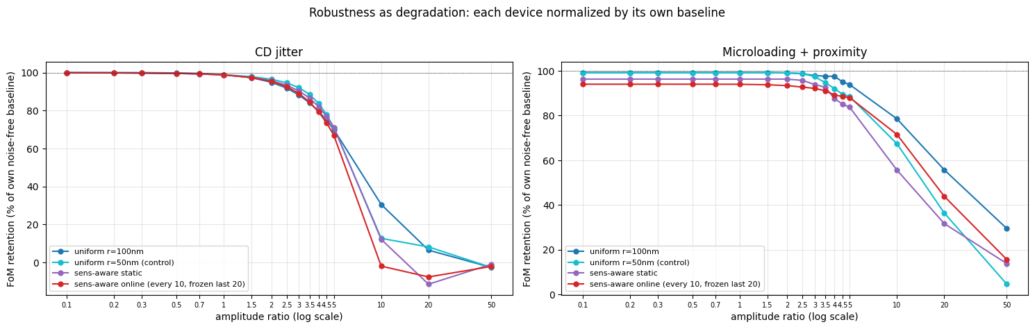
CD jitter: normalizing FLIPS the winner at ratios [0.1, 0.2, 0.3, 0.5, 0.7, 1, 1.5, 2, 2.5, 3, 3.5, 4, 4.5]
Microloading + proximity: normalizing FLIPS the winner at ratios [0.1, 0.2, 0.3, 0.5, 0.7, 1, 1.5, 3, 3.5, 4, 4.5, 5]

Note: retention is meaningless once the absolute FoM approaches zero (largest ratios) - read those columns from the absolute plot instead.
What changed. Under CD jitter the sens-aware "win" at the smallest amplitudes disappears: both devices retain >99% of their own baseline there, and uniform actually retains marginally more. The genuine sens-aware robustness advantage lives in a narrow middle band (ratio ≈ 1.5–5), not across the whole small-amplitude range.
Under microloading the correction is more severe: normalizing flips the winner at essentially every amplitude up to 4.5. Sens-aware led on absolute FoM only because it started 0.41 higher. Two things drive this — the constant offset from the binarization residual flagged earlier (sens-aware loses ~3.7% of baseline to re-binarization alone, uniform ~0.8%, independent of amplitude, which is why the smallest ratios are all identical), and a genuinely steeper decline past ratio 3.
So the submitted headline — "sens-aware wins on mean and variance at small-to-moderate amplitudes" — holds for CD jitter in a restricted window and does not hold for microloading at all once the baseline offset is removed.
(2) Paired analysis — CD jitter only
# CD jitter is exactly paired: identical rng(seed) noise field applied to both designs.
N_BOOT = 10000
_rng_boot = np.random.default_rng(0)
_pairs = [(RA_DEVS[i], RA_DEVS[j]) for i in range(len(RA_DEVS)) for j in range(i+1, len(RA_DEVS))]

fig, ax = plt.subplots(figsize=(10, 4.8))
for (d_a, d_b), _ls in zip(_pairs, ['-', '--', ':']):
    means, los, his = [], [], []
    for r in RATIOS:
        amp = CD_JITTER_BASE * r
        diff = (seed_sums(_RA[d_b]['cd'], amp) / _RA[d_b]['base']
                - seed_sums(_RA[d_a]['cd'], amp) / _RA[d_a]['base'])
        boot = np.array([diff[_rng_boot.integers(0, diff.size, diff.size)].mean()
                         for _ in range(N_BOOT)])
        lo, hi = np.percentile(boot, [2.5, 97.5])
        means.append(diff.mean()); los.append(lo); his.append(hi)
    means, los, his = 100*np.array(means), 100*np.array(los), 100*np.array(his)
    ax.plot(RATIOS, means, 'o-', ls=_ls, ms=4, color=DEV_COLORS[d_b],
            label=f"{DEV_LABELS[d_b]} − {DEV_LABELS[d_a]}")
    ax.fill_between(RATIOS, los, his, color=DEV_COLORS[d_b], alpha=0.18)
ax.axhline(0, color='black', lw=0.8)
ax.set_xscale('log'); ax.set_xticks(RATIOS)
ax.set_xticklabels([f"{x:g}" for x in RATIOS], fontsize=7)
ax.tick_params(axis='x', which='minor', bottom=False)
ax.set_xlabel('amplitude ratio (log scale)')
ax.set_ylabel('paired Δ retention (percentage points)')
ax.set_title(f"CD jitter: paired per-seed difference in FoM retention "
             f"({N_SAMPLES} seeds, {N_BOOT:,}× bootstrap, 95% CI)")
ax.grid(alpha=0.3); ax.legend(fontsize=8)
plt.tight_layout()
plt.show()

# Numeric table for the primary contrast.
d_a, d_b = 'uniform', ('sensaware' if 'sensaware' in RA_DEVS else RA_DEVS[-1])
print(f"CD jitter - paired delta retention, {DEV_LABELS[d_b]} − {DEV_LABELS[d_a]}")
print(f"{'ratio':>7}{'d (pp)':>10}{'95% CI (pp)':>24}{'sig':>6}{'seeds favouring':>17}")
for r in RATIOS:
    amp = CD_JITTER_BASE * r
    diff = (seed_sums(_RA[d_b]['cd'], amp) / _RA[d_b]['base']
            - seed_sums(_RA[d_a]['cd'], amp) / _RA[d_a]['base'])
    boot = np.array([diff[_rng_boot.integers(0, diff.size, diff.size)].mean()
                     for _ in range(N_BOOT)])
    lo, hi = np.percentile(boot, [2.5, 97.5])
    print(f"{r:>7g}{100*diff.mean():>+10.2f}[{100*lo:>+8.2f},{100*hi:>+8.2f}]"
          f"{('yes' if (lo>0)==(hi>0) else 'no'):>6}{(diff>0).sum():>13}/{diff.size}")
/var/folders/qn/syhrzy8n7930sgqvxv2x65s40000gn/T/ipykernel_33534/3336094999.py:18: UserWarning: linestyle is redundantly defined by the 'linestyle' keyword argument and the fmt string "o-" (-> linestyle='-'). The keyword argument will take precedence.
  ax.plot(RATIOS, means, 'o-', ls=_ls, ms=4, color=DEV_COLORS[d_b],
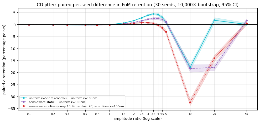
CD jitter - paired delta retention, sens-aware static − uniform r=100nm
  ratio    d (pp)             95% CI (pp)   sig  seeds favouring
    0.1     -0.08[   -0.08,   -0.08]   yes            0/30
    0.2     -0.14[   -0.15,   -0.14]   yes            0/30
    0.3     -0.19[   -0.20,   -0.18]   yes            0/30
    0.5     -0.25[   -0.26,   -0.24]   yes            0/30
    0.7     -0.25[   -0.27,   -0.23]   yes            0/30
      1     -0.16[   -0.20,   -0.12]   yes            2/30
    1.5     +0.22[   +0.14,   +0.30]   yes           25/30
      2     +0.82[   +0.69,   +0.97]   yes           30/30
    2.5     +1.53[   +1.31,   +1.76]   yes           30/30
      3     +2.16[   +1.85,   +2.47]   yes           30/30
    3.5     +2.51[   +2.12,   +2.94]   yes           30/30
      4     +2.49[   +1.97,   +3.02]   yes           30/30
    4.5     +2.04[   +1.42,   +2.69]   yes           29/30
      5     +1.14[   +0.40,   +1.89]   yes           18/30
     10    -18.42[  -19.99,  -16.79]   yes            0/30
     20    -17.95[  -19.19,  -16.73]   yes            0/30
     50     +1.61[   +0.88,   +2.32]   yes           24/30
What the pairing buys. The per-seed differences are far tighter than the marginal box widths, so effects of a fraction of a percentage point are resolved cleanly. The result is a sign-changing curve rather than a single crossover: sens-aware is significantly worse by 0.1–0.25 pp at ratios ≤ 1 (0/30 seeds favour it), significantly better by up to ~2.5 pp at ratios 2–4.5 (30/30 seeds favour it at ratios 2–4), and dramatically worse at ratios 10–20. Every one of those intervals excludes zero, so the shape is real and not seed noise — the effect is simply much smaller, and much more localized in amplitude, than the box plots imply.
(3) Peak shift vs. peak collapse, and the recentered FoM
_probe_ratios = [r for r in (1, 3, 5, 10, 50) if r in RATIOS] if _HAVE_MC else []
_rows = []

# Per-device spectrum sources: the originals share mc_spec; each extra device has its own.
_MC_CELLSRC = {d: MC_EXTRA[d]['spec']['cells'] for d in globals().get('MC_EXTRA', {})}
_ED_SRC     = {d: ED_EXTRA[d][1]              for d in globals().get('ED_EXTRA', {})}

if _HAVE_MC:
    for _mc_key, _base_amp in [('cdjitter', CD_JITTER_BASE), ('microloading', MICROLOADING_BASE)]:
        _cells = mc_spec['cells']
        for r in _probe_ratios:
            for dev in RA_DEVS:
                _cellsrc = _MC_CELLSRC.get(dev, _cells)
                key = f"{_mc_key}|{dev}|{_base_amp*r:g}"
                if key not in _cellsrc:
                    continue
                P = np.array(_cellsrc[key]['mean_T'])
                pk = port_peaks(P, ref_freqs)
                d, f_best, f_0 = best_recentering(P, ref_freqs)
                dl_nm = (1000*td.C_0/(float(np.mean(freqs_design)) + d)
                         - 1000*td.C_0/float(np.mean(freqs_design)))
                _rows.append(dict(
                    noise=_mc_key, ratio=r, dev=dev,
                    shift_nm=float(np.abs(pk[:,0] - REF_PEAKS[dev][:,0]).mean()),
                    drop_pp=float(100*(pk[:,1] - REF_PEAKS[dev][:,1]).mean()),
                    fom=f_0, fom_rc=f_best, best_dlam=dl_nm,
                    recovered=recovered_frac(f_best, f_0, _RA[dev]['base'])))

print(f"{'noise':>13}{'ratio':>7}{'device':>22} | {'|peak shift|':>13}{'peak drop':>11} | "
      f"{'FoM':>8}{'recentered':>11}{'best dlam':>11}{'recovered':>10}")
print("-" * 110)
for _r in _rows:
    print(f"{_r['noise']:>13}{_r['ratio']:>7g}{DEV_LABELS[_r['dev']]:>22} | "
          f"{_r['shift_nm']:>10.2f}nm{_r['drop_pp']:>10.1f}pp | {_r['fom']:>8.3f}"
          f"{_r['fom_rc']:>11.3f}{_r['best_dlam']:>+10.2f}nm  {fmt_recovered(_r['recovered'])}")

# ED sweep — one sim per point, so this is exact (no seed averaging).
print(f"\nErosion-dilation (exact, no seed averaging)")
print(f"{'amount':>8}{'device':>22} | {'peak shift':>13}{'peak drop':>11} | "
      f"{'FoM':>8}{'recentered':>11}{'best dlam':>11}{'recovered':>10}")
print("-" * 105)
_ed_rows = []
for amt in ED_AMOUNTS_NM:
    for dev in RA_DEVS:
        _src = _ED_SRC.get(dev, ed_spec)
        key = f"{dev}|{amt:+g}"
        if key not in _src['cells']:
            continue
        P = np.array(_src['cells'][key]['T'])
        F = np.array(_src['freqs'])
        pk = port_peaks(P, F)
        d, f_best, f_0 = best_recentering(P, F)
        dl_nm = (1000*td.C_0/(float(np.mean(freqs_design)) + d)
                 - 1000*td.C_0/float(np.mean(freqs_design)))
        rec = recovered_frac(f_best, f_0, _RA[dev]['base'])
        _ed_rows.append(dict(amt=amt, dev=dev, fom=f_0, fom_rc=f_best, recovered=rec))
        if amt % 4 == 0:
            print(f"{amt:>+7g}nm{DEV_LABELS[dev]:>22} | "
                  f"{(pk[:,0]-REF_PEAKS[dev][:,0]).mean():>+10.2f}nm"
                  f"{100*(pk[:,1]-REF_PEAKS[dev][:,1]).mean():>10.1f}pp | "
                  f"{f_0:>8.3f}{f_best:>11.3f}{dl_nm:>+10.2f}nm  {fmt_recovered(rec)}")
        noise  ratio                device |  |peak shift|  peak drop |      FoM recentered  best dlam recovered
--------------------------------------------------------------------------------------------------------------
     cdjitter      1       uniform r=100nm |       0.67nm      -0.5pp |    3.363      3.364     -0.35nm      3.0%
     cdjitter      1uniform r=50nm (control) |       1.32nm      -0.5pp |    3.670      3.696     -1.05nm     63.7%
     cdjitter      1     sens-aware static |       1.16nm      -0.7pp |    3.761      3.778     -1.05nm     36.9%
     cdjitter      1sens-aware online (every 10, frozen last 20) |       1.49nm      -0.1pp |    2.773      2.802     -1.05nm     82.5%
     cdjitter      3       uniform r=100nm |       2.82nm      -2.9pp |    2.998      3.046     -1.05nm     12.1%
     cdjitter      3uniform r=50nm (control) |       4.91nm      -2.1pp |    3.416      3.622     -3.66nm     69.8%
     cdjitter      3     sens-aware static |       5.98nm      -3.0pp |    3.440      3.670     -3.66nm     62.7%
     cdjitter      3sens-aware online (every 10, frozen last 20) |       4.93nm      -1.0pp |    2.499      2.756     -4.36nm     83.3%
     cdjitter      5       uniform r=100nm |       3.77nm      -8.1pp |    2.379      2.547     -2.97nm     16.5%
     cdjitter      5uniform r=50nm (control) |       7.87nm      -4.8pp |    2.635      3.493     -6.27nm     79.7%
     cdjitter      5     sens-aware static |       8.78nm      -5.6pp |    2.708      3.536     -6.44nm     75.4%
     cdjitter      5sens-aware online (every 10, frozen last 20) |       6.77nm      -1.6pp |    1.879      2.703     -6.96nm     88.8%
     cdjitter     10       uniform r=100nm |       6.68nm     -41.6pp |    1.036      1.058     +1.58nm      0.9%
     cdjitter     10uniform r=50nm (control) |      14.78nm     -16.9pp |    0.468      2.839    -12.31nm     73.1%
     cdjitter     10     sens-aware static |      15.01nm     -13.0pp |    0.460      3.158    -12.99nm     80.6%
     cdjitter     10sens-aware online (every 10, frozen last 20) |      12.60nm      -8.0pp |   -0.057      2.154    -12.99nm     77.2%
     cdjitter     50       uniform r=100nm |      17.68nm     -81.8pp |   -0.091      0.054    +14.15nm      4.1%
     cdjitter     50uniform r=50nm (control) |      18.05nm     -85.7pp |   -0.099      0.078    -13.51nm      4.6%
     cdjitter     50     sens-aware static |      13.05nm     -90.5pp |   -0.040     -0.028     -3.66nm      0.3%
     cdjitter     50sens-aware online (every 10, frozen last 20) |      12.37nm     -66.3pp |   -0.062     -0.019    -13.68nm      1.5%
 microloading      1       uniform r=100nm |       0.51nm      -0.1pp |    3.371      3.385     +0.88nm     48.8%
 microloading      1uniform r=50nm (control) |       0.49nm      -0.8pp |    3.678      3.679     -0.35nm      1.2%
 microloading      1     sens-aware static |       1.36nm      -1.5pp |    3.665      3.689     +1.58nm     17.0%
 microloading      1sens-aware online (every 10, frozen last 20) |       0.99nm      -2.0pp |    2.638      2.644     +0.35nm      3.8%
 microloading      3       uniform r=100nm |       0.68nm      -0.9pp |    3.325      3.339     +0.88nm     18.7%
 microloading      3uniform r=50nm (control) |       1.00nm      -2.5pp |    3.613      3.614     -0.35nm      1.0%
 microloading      3     sens-aware static |       1.34nm      -4.3pp |    3.573      3.588     +1.58nm      6.3%
 microloading      3sens-aware online (every 10, frozen last 20) |       0.82nm      -3.3pp |    2.586      2.592     +0.35nm      2.6%
 microloading      5       uniform r=100nm |       1.37nm      -4.2pp |    3.189      3.199     +0.88nm      4.8%
 microloading      5uniform r=50nm (control) |       1.98nm     -10.4pp |    3.284      3.284     -0.35nm      0.1%
 microloading      5     sens-aware static |       2.67nm     -13.2pp |    3.186      3.199     +0.88nm      2.1%
 microloading      5sens-aware online (every 10, frozen last 20) |       1.84nm      -6.0pp |    2.471      2.478     +0.35nm      1.9%
 microloading     10       uniform r=100nm |       1.36nm     -17.1pp |    2.669      2.678     +0.88nm      1.3%
 microloading     10uniform r=50nm (control) |       4.40nm     -27.3pp |    2.500      2.503     -0.35nm      0.3%
 microloading     10     sens-aware static |       2.16nm     -36.1pp |    2.116      2.130     +1.58nm      0.8%
 microloading     10sens-aware online (every 10, frozen last 20) |       1.82nm     -16.5pp |    2.008      2.012     +0.35nm      0.5%
 microloading     50       uniform r=100nm |       2.24nm     -59.2pp |    1.001      1.001     +0.18nm      0.0%
 microloading     50uniform r=50nm (control) |       7.32nm     -84.9pp |    0.170      0.191     +5.62nm      0.6%
 microloading     50     sens-aware static |       6.75nm     -77.3pp |    0.525      0.526     +0.88nm      0.0%
 microloading     50sens-aware online (every 10, frozen last 20) |      10.62nm     -53.2pp |    0.438      0.438     -0.35nm      0.0%

Erosion-dilation (exact, no seed averaging)
  amount                device |    peak shift  peak drop |      FoM recentered  best dlam recovered
---------------------------------------------------------------------------------------------------------
     -8nm       uniform r=100nm |      -8.17nm      -1.4pp |    2.208      3.298     -7.14nm     91.6%
     -8nmuniform r=50nm (control) |      -9.78nm      -3.0pp |    1.272      3.470     -9.55nm     90.1%
     -8nm     sens-aware static |     -11.03nm      -1.6pp |    1.756      3.702     -8.35nm     94.9%
     -8nmsens-aware online (every 10, frozen last 20) |     -10.05nm      -2.1pp |    1.021      2.651     -9.55nm     91.3%
     -4nm       uniform r=100nm |      -2.34nm      -0.0pp |    3.313      3.390     -1.75nm     89.4%
     -4nmuniform r=50nm (control) |      -4.00nm      -1.1pp |    3.461      3.654     -3.14nm     77.4%
     -4nm     sens-aware static |      -2.47nm      -1.1pp |    3.639      3.714     -1.75nm     44.9%
     -4nmsens-aware online (every 10, frozen last 20) |      -4.14nm      -1.6pp |    2.460      2.666     -2.97nm     59.3%
     +0nm       uniform r=100nm |      +0.00nm       0.0pp |    3.399      3.399     +0.35nm       n/a
     +0nmuniform r=50nm (control) |      +0.00nm       0.0pp |    3.711      3.711     -0.35nm       n/a
     +0nm     sens-aware static |      +0.00nm       0.0pp |    3.807      3.807     +0.18nm       n/a
     +0nmsens-aware online (every 10, frozen last 20) |      +0.00nm       0.0pp |    2.808      2.808     +0.18nm       n/a
     +4nm       uniform r=100nm |      +2.51nm      -0.7pp |    3.161      3.349     +3.51nm     79.1%
     +4nmuniform r=50nm (control) |      +2.36nm      -1.0pp |    3.582      3.667     +2.98nm     66.0%
     +4nm     sens-aware static |      +3.06nm      -2.3pp |    3.381      3.651     +4.21nm     63.4%
     +4nmsens-aware online (every 10, frozen last 20) |      +1.82nm      -2.6pp |    2.560      2.609     +2.28nm     19.6%
     +8nm       uniform r=100nm |      +7.52nm      -2.6pp |    2.056      3.201     +7.75nm     85.3%
     +8nmuniform r=50nm (control) |      +7.52nm      -2.3pp |    2.037      3.596     +7.75nm     93.2%
     +8nm     sens-aware static |      +7.64nm      -5.1pp |    1.792      3.541     +8.99nm     86.8%
     +8nmsens-aware online (every 10, frozen last 20) |      +7.16nm      -4.5pp |    1.618      2.516     +7.75nm     75.5%
# FoM as-measured vs recentered, CD jitter and microloading.
fig, axes = plt.subplots(1, 3, figsize=(17, 4.4))
for ax, _mc_key, _base_amp, _title in [
        (axes[0], 'cdjitter',     CD_JITTER_BASE,    'CD jitter'),
        (axes[1], 'microloading', MICROLOADING_BASE, 'Microloading + proximity')]:
    for dev in RA_DEVS:
        sel = [r for r in _rows if r['noise'] == _mc_key and r['dev'] == dev]
        if not sel:
            continue
        xs = [r['ratio'] for r in sel]
        ax.plot(xs, [r['fom']    for r in sel], 'o--', color=DEV_COLORS[dev], alpha=0.5,
                label=f"{DEV_LABELS[dev]} (as measured)")
        ax.plot(xs, [r['fom_rc'] for r in sel], 'o-',  color=DEV_COLORS[dev],
                label=f"{DEV_LABELS[dev]} (recentered)")
    ax.set_xscale('log'); ax.set_xlabel('amplitude ratio'); ax.set_ylabel('FoM')
    ax.set_title(_title); ax.grid(alpha=0.3); ax.legend(fontsize=7)
for dev in RA_DEVS:
    sel = [r for r in _ed_rows if r['dev'] == dev]
    axes[2].plot([r['amt'] for r in sel], [r['fom']    for r in sel], 'o--',
                 color=DEV_COLORS[dev], alpha=0.5, label=f"{DEV_LABELS[dev]} (as measured)")
    axes[2].plot([r['amt'] for r in sel], [r['fom_rc'] for r in sel], 'o-',
                 color=DEV_COLORS[dev], label=f"{DEV_LABELS[dev]} (recentered)")
axes[2].set_xlabel(r'$\Delta$ (nm)'); axes[2].set_ylabel('FoM')
axes[2].set_title('Erosion-dilation'); axes[2].grid(alpha=0.3); axes[2].legend(fontsize=7)
fig.suptitle("As-measured (dashed) vs wavelength-recentered (solid) FoM", y=1.02)
plt.tight_layout()
plt.show()
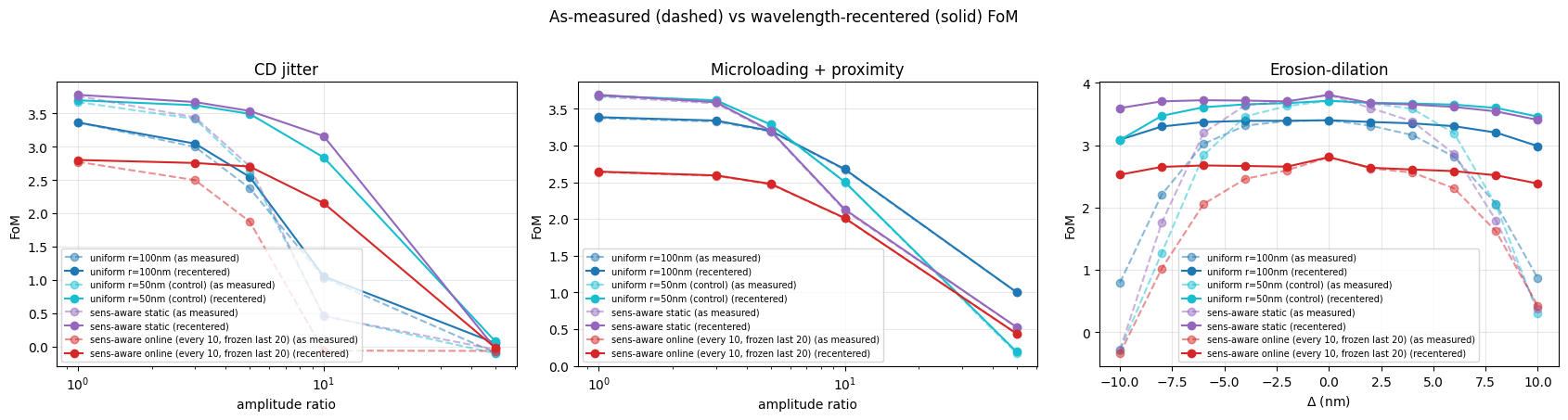
The hypothesis holds — for CD jitter, and decisively. The decomposition confirms the mechanism that was previously only asserted from eyeballing the spectra. At CD-jitter ratio 10 the uniform device's peaks collapse by −41.6 pp while shifting only 6.7 nm; the sens-aware device's peaks drop just −13.0 pp but shift 15.0 nm. Recentering the channel bands on a single global $\delta\lambda$ recovers 80.6% of the sens-aware device's lost FoM and 0.9% of the uniform device's. The verdict inverts: as measured, uniform leads $1.04$ vs $0.46$; recentered, sens-aware leads $3.16$ vs $1.06$. The large-amplitude crossover reported in the box plots is therefore substantially an artifact of a band-fixed metric, exactly as the Discussion speculated — and the effect is larger than expected, since the mean-spectrum smearing means these are lower bounds.
It does not generalize to microloading. There, recentering recovers almost nothing for either device (≤2% past ratio 3), and the sens-aware device's peak drop is consistently worse than uniform's (−36.1 pp vs −17.1 pp at ratio 10). Under feature-size-dependent morphological error, sens-aware genuinely fails by peak collapse, not by detuning. The "it's only a wavelength shift" defence is specific to spatially-uncorrelated edge noise.
Erosion-dilation is almost pure detuning for both devices. Recentering recovers 80–95% of the loss on both at $|\Delta| \geq 6$ nm — unsurprising, since a uniform boundary bias is close to an effective-index change. It does not discriminate between the filters, though sens-aware retains the higher recentered FoM at the sweep extremes.
Practical reading. If the deployment can tolerate a global channel-grid re-spec after fab characterization — which is routine for a CWDM demux — the sens-aware device is the better choice out to far larger CD-jitter amplitudes than the box plots suggest. If the channel grid is fixed by spec, the box-plot reading stands.
New sweeps: the schedule variant and the control / online robustness
The comparison now carries five devices — the original uniform $r{=}100$ nm and sens-aware static, plus the $r{=}50$ nm control, the every-step online filter, and a schedule variant (refresh every 10 steps up to step 30, then frozen for the final 20). Everything below renders from cache; no new simulations were run.
Noise-free ordering is unchanged by the new data. Sum-FoM baselines: uniform $r{=}100$ nm $+3.399$, $r{=}50$ nm control $+3.711$, sens-aware static $+3.807$, online (every step) $+2.096$, schedule $+2.808$. The control decomposition holds: of the static filter's gain over uniform-100, 78% is the finer floor ($\text{u50}-\text{u100}$) and only 22% is sensitivity reallocation ($\text{static}-\text{u50}$).
Both online variants fail as four-channel demuxes. Port 3 transmits $\sim0.1\%$ for both the every-step (mean 55.3%) and schedule (mean 70.8%) devices — one channel is effectively dead, so their FoM is carried by three ports. The online refresh, in either form, does not produce a working device on this problem.
Scheduling the refresh recovers part of the every-step loss. Freezing the blend map once $\beta$ is large lifts training $J$ from $-1.217$ (every step) to $-1.005$ (schedule) and restores the trajectory — 82% monotonic steps vs 55% (static is 86%). That recovers 39% of the every-step-to-static gap, partial support for the edge-peaked-gradient hypothesis in the Discussion: the refresh is most damaging late in training, when the projection derivative concentrates the gradient on the material boundary.
Erosion-dilation retention (new sweeps, every device). Mean own-baseline retention over $\pm10$ nm: uniform-100 75.8%, control 67.1%, static 66.4%, online every-step 72.1%, schedule 65.2%. The every-step online device's higher retention is retention of an already-degraded device — its absolute FoM stays far below the working devices — so it is not evidence of real robustness. As under CD jitter, the coarsest device (uniform-100) retains the most.
Net. The new sweeps reinforce the revised verdict rather than overturn it: the mechanism's nominal contribution is small (22% of the static gain), the every-step online refresh is harmful, and scheduling it recovers part but not all of the loss while still leaving one channel dead.
Discussion
Summary of findings. The original three claims were measured against a uniform $r = 100$ nm baseline. With the matched-floor $r = 50$ nm control now trained, two of the three do not survive:
-
Nominal FoM: 77% of the gain was the finer floor, not the mechanism. Sum-FoM is 3.399 (uniform 100 nm) → 3.711 (50 nm control) → 3.807 (adaptive). Of the $+0.408$ originally credited to sensitivity-driven filtering, $+0.312$ is the floor and only $+0.096$ is reallocation — and that residual is a single training seed with no error bar.
-
Robustness: the plain 50 nm control is more robust than the adaptive filter. On own-baseline retention the adaptive filter wins at 6/17 CD-jitter amplitudes and 1/17 microloading amplitudes, losing across the entire physically realistic mid-range. The adaptive filter buys no robustness over a plain uniform filter at the same floor.
There is no simple feature-size law here. On absolute FoM the uniform 100 nm device is the worst of the three at every amplitude from ratio 0.1 to 5 — it loses to the 50 nm control on 0 of 30 seeds at ratio 5 — and fitting $J(\sigma) = J_0 - c\sigma^2$ in the small-noise regime gives it the largest curvature ($c = 450$ against 317 for the 50 nm control and 401 for the adaptive device). The finer-floor devices are both higher-performing and sitting in flatter optima. The single exception is CD-jitter ratio 10, where the 100 nm device wins decisively (1.036 vs 0.468, 30/30 seeds); by ratio 20 the ordering reverses again. That one bin is discussed below and is unexplained.
-
The "routes around hot spots" claim is a boundary-length artifact. Fraction of material boundary in the top sensitivity decile (chance = 10%): uniform 100 nm 22.0%, control 11.3%, adaptive 11.0%. The control carries no sensitivity information whatsoever and reproduces the adaptive design's number. Both 50 nm-floor devices have ~40% more boundary, which dilutes the statistic toward chance.
What does survive. The adaptive run has the most monotonic trajectory of everything trained — 86% of steps improving, against 71% for the control and 63% for the baseline. Feature size does not explain that, since the control shares the floor. The claim that the adaptive filter gives the optimizer a smoother landscape appears real even though the converged advantage is small.
Why the effect is so small. Under $\max$ normalization the sensitivity field is heavy-tailed enough that the median effective radius is 50.3 nm and only 0.12% of pixels exceed blend 0.5 — the "adaptive" filter is a uniform 50 nm filter over 99.9% of the design region. This study has therefore not really tested spatial reallocation; it has tested a 50 nm uniform filter with a rounding error on top.
The unexplained bin. At CD-jitter ratio 10 the uniform 100 nm device retains far more FoM than either 50 nm-floor device (1.036 vs 0.468 and 0.460, on 30/30 seeds — the effect is not seed noise). Recentring the channel bands on a single global $\delta\lambda$ recovers 73% of the 50 nm control's loss and 81% of the adaptive device's, but only 0.9% of the 100 nm device's: the two fine-floor devices coherently detune by ~12–13 nm, while the coarse one does not detune at all. We tested three mechanisms for that and all three failed:
| proposed mechanism | prediction | measured |
|---|---|---|
| more boundary ⟹ noise bites harder | larger realized $\Delta\rho$ | rms $\Delta\rho$ = 0.0714 / 0.0711 / 0.0713 — identical |
| coarse device has broader passbands | 100 nm widest | mean FWHM 20.1 / 18.7 / 21.4 nm — the adaptive device is widest |
the shift is argmax noise on degraded spectra |
recentring should not help | it recovers 73–81% for the fine devices — the shift is real |
Nor is it general phase sensitivity: under erosion-dilation, a coherent geometric perturbation, the 100 nm and adaptive devices detune at nearly the same rate ($-8.2$ vs $-11.0$ nm at $\Delta = -8$ nm). The 100 nm device is not stiff against index perturbations in general — it simply does not respond to this particular one.
Note also that the $r = 50$ nm control and the adaptive device are indistinguishable on every measure here — FoM at ratio 10 (0.468 vs 0.460), detuning (14.8 vs 15.0 nm), recovery (73% vs 81%), boundary pixels (12,059 vs 12,495), realized perturbation. So whatever separates the 100 nm device has nothing to do with the sensitivity filter.
With one converged design per filter condition, an effect confined to a single amplitude bin, correlating with none of the available structural metrics and reversing the ordering seen at every other amplitude, is what a device-specific geometric accident looks like. We cannot distinguish "100 nm filtering causes this" from "this particular geometry does this" without multiple seeds. It should be read as an unexplained observation, not a feature-size law.
Robustness. Under stochastic fab error (CD jitter, microloading + proximity), the sensitivity-aware device wins on both mean FoM and FoM variance at small-to-moderate amplitudes. At very large amplitudes the box-plot FoM flips to the uniform device — but this is partly an artifact of the metric: the per-port spectra reveal that the sensitivity-aware device's failure mode at large amplitudes is a wavelength shift of an otherwise-intact peak, while the uniform device's failure mode is a drop in peak height. A wavelength-recentered FoM would extend the sensitivity-aware win-rate further into the large-amplitude regime.
Online (per-iteration) filter updates — and why they failed. The static filter is bootstrapped once from the uniform-converged sensitivity field and then frozen, so by late training it modulates on a stale map. The online variant rebuilds the blend map from the gradient the optimizer computes at every Adam step, at zero additional simulation cost. It performed much worse than everything else:
| device | sum-FoM | monotonic steps | mean $r_{\rm eff}$ |
|---|---|---|---|
| uniform r=50nm (control) | 3.711 | 71% | 50 nm |
| sens-aware static (max-norm, frozen) | 3.807 | 86% | 51.3 nm |
| sens-aware online, $\partial J/\partial\rho$ | 1.377 | 57% | 60.1 nm |
| sens-aware online, $\partial J/\partial\bar\rho$ | 2.096 | 55% | 61.7 nm |
Normalization alone cannot explain this. The online runs used p99 normalization and the static run used $\max$, so their filters were coarser — mean effective radius ~60 nm against ~51 nm. But feature size is a smooth, well-behaved axis here: a uniform 100 nm filter scores 3.399 and a uniform 50 nm filter scores 3.711, so a filter with ~60 nm mean radius should interpolate to roughly 3.6, not 1.4–2.1. The online runs fall about 1.5–2.3 sum-FoM below what their effective feature size predicts. Something about the refresh itself is damaging, and the confound with normalization — real, and a reason not to over-read the exact numbers — is nowhere near large enough to account for the gap.
Five hypotheses, ordered by how well they fit the evidence:
- The gradient becomes edge-peaked as $\beta$ anneals, so the filter coarsens exactly the features it should be sharpening. $\partial J/\partial\rho = \mathcal{F}^{\top}(\partial J/\partial\bar\rho \odot \mathrm{proj}')$, and the projection derivative $\mathrm{proj}' \sim \beta\,\mathrm{sech}^2(\beta(\rho - 0.5))$ is sharply peaked at the material boundary — increasingly so as $\beta$ ramps 1 → 50. Normalizing an edge-peaked field drives blend → 1 on the contour, which applies $r_{\rm high} = 150$ nm precisely at the boundaries the optimizer is trying to resolve. The filter then fights the $\beta$ anneal, and does so harder every iteration. This predicts the observed ordering: $\partial J/\partial\bar\rho$ carries no $\mathrm{proj}'$ factor and is therefore less edge-dominated, and it scored +0.72 higher than $\partial J/\partial\rho$. It also predicts the damage is concentrated late in training, when $\beta$ is large.
- A non-stationary objective invalidates Adam's moment estimates. Adam's first and second moments are running averages that assume a fixed objective. Refreshing the filter changes the map $\rho \mapsto \bar\rho \mapsto J$, i.e. it changes the objective function itself, every single step. The accumulated moments then describe the curvature of a function that no longer exists, and the effective step size is systematically wrong. This fits the collapse in trajectory quality — 55–57% monotonic steps against 71% for the control and 86% for static.
- The geometry jumps between the gradient and its use. At step $k$ we compute $\nabla J$ under filter $F_k$, apply the parameter update, then evaluate under $F_{k+1}$. The gradient describes how $J$ moves when $\rho$ changes with the filter held fixed; the design actually evaluated next has a different filter. Worse, refreshing changes $\bar\rho$ even with $\rho$ untouched, so at every refresh the device geometry moves with no optimizer step behind it. Under $\max$ normalization those jumps are negligible (blend ≈ 0 everywhere, which is why static is unharmed); under p99 the map has real structure and the jumps are not.
-
Feedback contamination of the map (the $\partial J/\partial\rho$ variant specifically). Because the backward pass runs through the current blend map, the map partly determines its own successor. Measured by pushing an identical physical sensitivity through an all-$r_{\rm low}$ versus an all-$r_{\rm high}$ map: the resulting maps correlate at only 0.454, with a mean absolute difference (0.089) larger than the mean blend value itself (0.073). This is the one hypothesis already confirmed by direct measurement, and it is why
SENS_WRTdefaults to"density". - The bootstrap seed is meaningless at the gray initialization. Both variants seed from a converged device's sensitivity field, then apply it to $\rho = 0.5\cdot\mathbf{1}$. For the static filter that mismatch is harmless because the map is ≈ 0 everywhere. The online filter replaces it at step 1 with the actual gradient at a uniform gray design — a diffuse, large-scale field with no relation to any final geometry — and commits the run to that map during the critical early binarization phase.
A sixth possibility we can rule out. The refresh was not simply too weak to matter: mean effective radius moved only 57.1 → 56.7 nm and 55.0 → 57.4 nm over fifty steps, so in aggregate the map barely drifted. But aggregate drift is the wrong statistic — hypotheses 1 and 3 are about where the map sits, not how far its mean travels, and a map that stays edge-locked while the edges move is doing damage at constant mean radius.
Diagnostics that would separate these, all cheap and mostly free: log $\|\bar\rho(\rho_k, b_k) - \bar\rho(\rho_k, b_{k+1})\|$ per step to size the refresh-induced geometry jump directly (hypothesis 3, zero sims); plot blend against distance to the 0.5 contour at low and high $\beta$ (hypothesis 1, zero sims — the snapshots are already cached); re-run with the filter frozen after $\beta$ exceeds ~20, which should recover most of the loss if hypothesis 1 dominates (one training run); and re-run with Adam's state reset at each refresh, or with plain gradient descent, to test hypothesis 2 (one training run).
The honest position is that the online variant is untested rather than refuted: it was run at a different normalization from its comparator, and the leading hypothesis suggests it may be fixable by not refreshing late in training.
Caveats.
- The blend map is far more one-sided than it looks. Under $\max$ normalization the uniform-converged sensitivity field is so heavy-tailed that the median effective radius is ~50 nm and fewer than 0.2% of pixels exceed blend 0.5 — the static "adaptive" filter is, for almost every pixel, simply a uniform 50 nm filter. This is quantified in the diagnostic cell at the top of the online section. It is why the online runs default to percentile normalization, which actually exercises both radii, and it is what motivated the $r = 50$ nm control below.
-
Same design freedom? This now has a control. The adaptive filter has $r_{\rm low} = 50$ nm $< 100$ nm $= r_{\rm uniform}$, so part of any win is raw extra design freedom rather than spatial reallocation. The "Control: uniform filter at $r = 50$ nm" section trains that exact ablation, and the four-way training cell prints the decomposition: how much of the reported static gain is the finer floor alone (
u50 − u100) versus sensitivity-driven reallocation on top (static − u50). Read that split before quoting any adaptive-vs-uniform number — the headline $r = 100$ nm comparison overstates the mechanism's contribution by whatever the first term is. -
Which sensitivity variable. The filter is now driven by $\partial J/\partial\bar\rho$ — sensitivity to the manufactured density — rather than $\partial J/\partial\rho$, which is that quantity smeared back through the filter kernel. The old choice was both physically wrong for the stated motivation and, for the online variant, self-referential: holding the physical sensitivity fixed and pushing it through an all-$r_{\rm low}$ versus an all-$r_{\rm high}$ blend map produced maps correlated at only 0.454.
SENS_WRT = "params"reproduces the old behaviour for comparison. The static device predates this fix and its caches encode the $\partial J/\partial\rho$ bootstrap; it is left unchanged rather than silently re-run, so a static-vs-online comparison should useSENS_WRT = "params"to keep the refresh as the only variable. - Estimator, not just variable. Park et al. use integrated gradients — the gradient averaged along a path from a baseline mask — which handles saturation in a way a single-point gradient does not. Switching to $\partial J/\partial\bar\rho$ matches their attribution variable but not their estimator. Matching the estimator would cost one forward+adjoint per path point (10–50× per refresh) and would destroy the "free at every Adam step" property that makes the online variant worth doing at all.
- One seed, one device. Every run here is a single optimization from a deterministic $\rho = 0.5$ init. Topology optimization is multi-modal and run-to-run spread across inits can be comparable to the gaps being reported, so none of these differences has an error bar on the training side. (The Monte-Carlo robustness numbers do have seed statistics; the converged-FoM comparisons do not.) Three to five perturbed inits per filter condition would turn each converged $J$ from a point into a distribution, and is the cheapest way to establish that the ordering is real.
- Foundry design rules. The smallest features in our sens-aware design (~76 nm) sit below the 100 nm penalty radius the original tutorial used; a foundry with a strict 100 nm design rule would need a tighter $r_{\rm low}$.
- Sensitivity field is bootstrapped. We use the uniform-converged sensitivity field as a fixed input to the adaptive filter for the entire sens-aware run. Updating the filter live during training (since $\partial J/\partial \rho$ is computed every step anyway) is the obvious upgrade — see Next steps.
- Microloading binarization residual (already flagged in the section intro): the per-feature morphological model re-binarizes via $\rho > 0.5$, costing ~3% of baseline FoM for the sens-aware design and <1% for the uniform device, independent of perturbation amplitude. The relative comparison is unaffected.
Next steps.
- Multi-seed runs. The single most valuable remaining experiment: 3–5 perturbed inits per filter condition, so the converged-$J$ comparisons carry error bars. At ~50 sims per run this is the difference between "A beat B once" and a measured effect.
- Robust TO as the baseline. Everything here is compared against non-robust topology optimization, which is a weak reference — the standard baseline for robustness claims is three-corner robust TO (erode/nominal/dilate worst-case), and that costs 3× forward+adjoint per iteration where the adaptive filter costs 1×. If the sensitivity-driven filter matches three-corner robustness at a third of the optimization cost, that is a far more actionable claim than beating vanilla TO, and it needs one 150-sim run to establish.
-
Normalization ablation and a bootstrap-free online run. Two loose ends from the online section: (a) re-run the static filter under percentile normalization, so that static-vs-online is a single-variable comparison at matched modulation strength; and (b) seed the online filter from a neutral map instead of the uniform-converged field, which would make the method fully self-contained — no bootstrap uniform run required at all.
ONLINE_NORMand theseed_sensitivityargument oftrain_onlineare the two knobs; both runs are 50 sims each. -
Update cadence sweep.
UPDATE_EVERYis exposed but only $K = 1$ is characterized here. If the every-step refresh proves noisy early in training (when the gradient field is spikiest), $K \in \{5, 10\}$ or an EMA over recent gradient fields would smooth the map at no extra cost. - More functionals, more channels. If the WDM is given more channels (or, more generally, if the design objective has more spectral targets), the device must produce tighter per-channel peaks → higher Q resonators → finer required feature sizes. We hypothesize that the sensitivity-aware vs uniform gap grows in this regime: the uniform filter's single global feature-size floor becomes harder to satisfy uniformly, while the adaptive filter relaxes the floor exactly where the adjoint says it's safe.
- Higher-Q test devices. Bragg-style filters, photonic-crystal cavities, ring-coupled wavelength filters — devices where sub-wavelength resonant features are load-bearing, not just useful — are the cleanest test of the mechanism. On those devices, the uniform filter doesn't just reallocate design budget; it blocks essential features outright. The sensitivity-aware filter should open up design space the uniform filter forbids.
References
- Junho Park, Taehan Kim, Mohammad Ali, Di Liang. Interpretable Geometry Sensitivity for Inverse Design of Integrated Photonics. arXiv:2510.22176, 2025. — the attribution target we follow: their surrogate maps binary masks to transmission and their validation perturbs physical pixels, which is why the filter here is driven by $\partial J/\partial\bar\rho$ rather than $\partial J/\partial\rho$.
- M. Schevenels, B. S. Lazarov, O. Sigmund. Robust topology optimization accounting for spatially varying manufacturing errors. Computer Methods in Applied Mechanics and Engineering, 2011.
- M. Sundararajan, A. Taly, Q. Yan. Axiomatic Attribution for Deep Networks. ICML 2017.
- Flexcompute, Inc.
tidy3d.plugins.invdesdocumentation: Autograd9WDM tutorial.

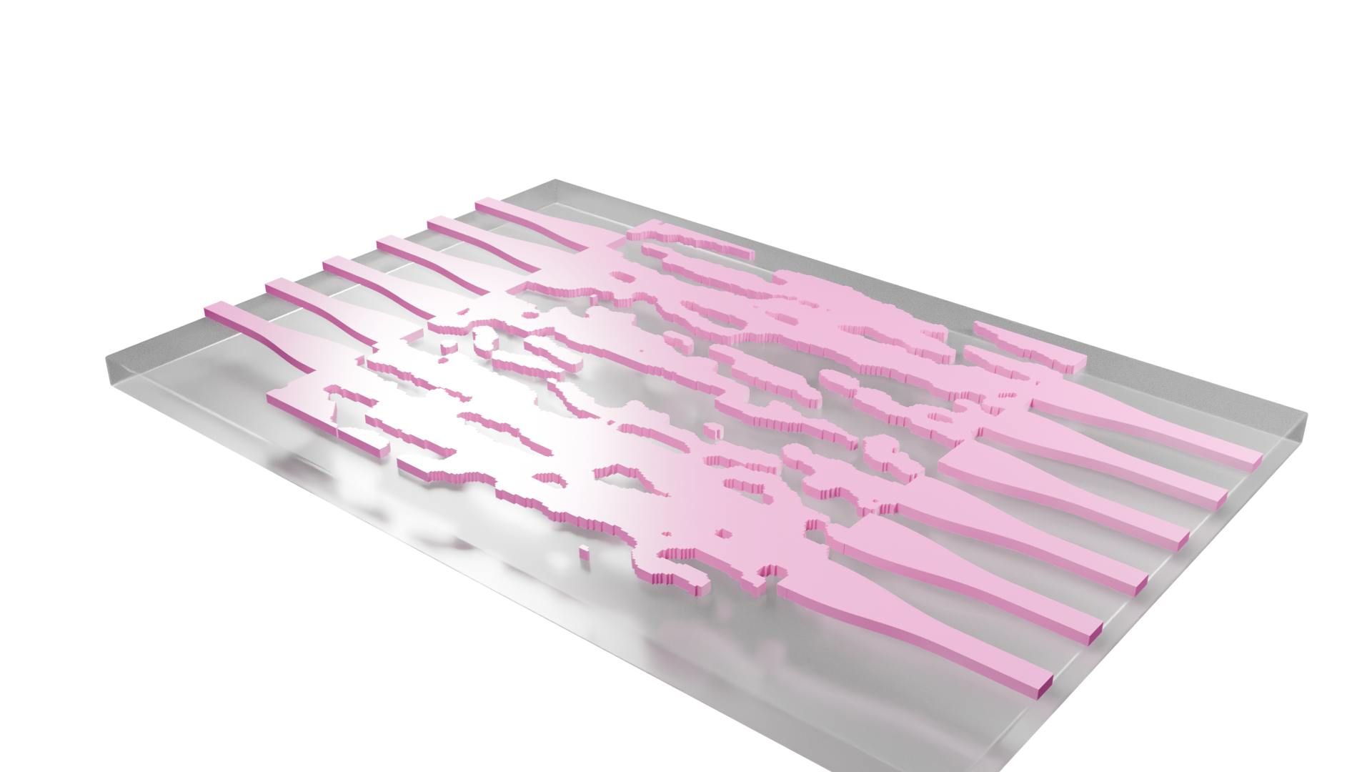


 TERMS & CONDITIONS


 How the process works:
 Try this real URL to see an example: