Author: Sumaia Jahan Mishu, The University of Oklahoma

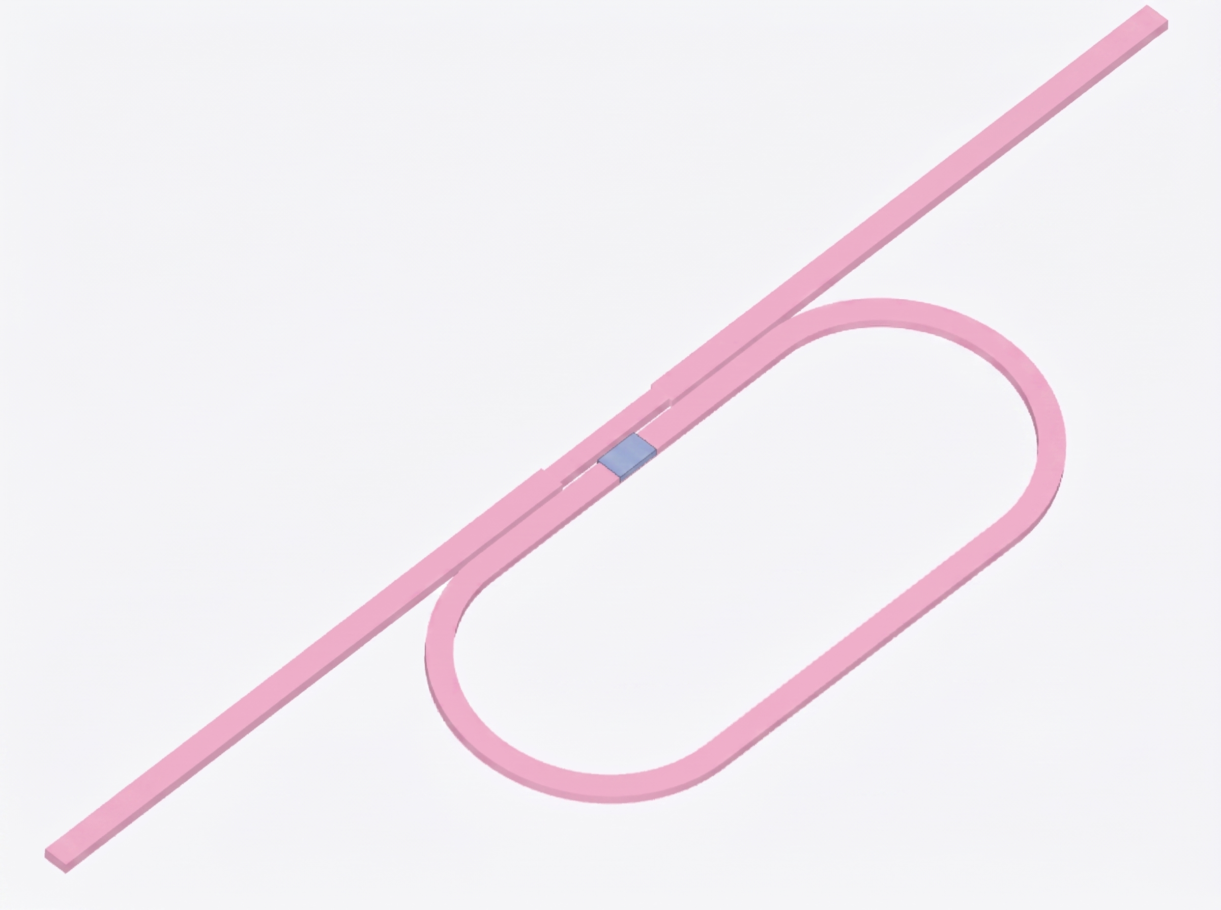
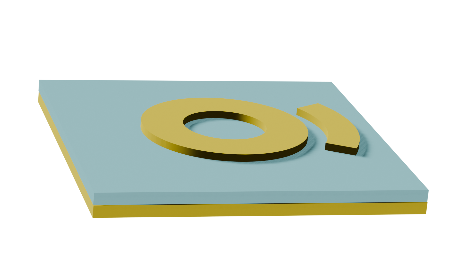
This Community Library notebook develops a silicon bus-coupled racetrack resonator with a nanoscale GST phase-change patch into a calibrated programmable optical-weight element using Tidy3D.

The workflow covers:

3D FDTD modeling of the racetrack coupler.
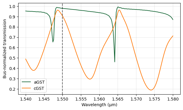
Optimized aGST/cGST transmission contrast near 1.55 µm.
Fixed-state optical linearity.
Bruggeman effective-medium modeling of intermediate GST states.
Dense (T(\lambda,x)) calibration and inverse weight mapping.
Scalar optical multiplication.
ITO-heater optical-penalty analysis.
Literature-parameterized electrothermal + JMAK write-path modeling.
Four-level write-verify.
Robust multilevel separation and effective bit depth.

Related Tidy3D examples:

If you are new to FDTD, see FDTD 101. If a simulation diverges, follow the troubleshooting guide.

Claim boundary: Optical FDTD results are simulation based. The heater electrothermal and GST-kinetics sections are design-exploration models, not fabrication recipes or measured device data.

FlexCredit note: Cloud execution is disabled by default. Set RUN_CLOUD=True only after inspecting the simulation and checking cost.

No description has been provided for this image

1. Imports¶

[1]:

from pathlib import Path
import numpy as np
import pandas as pd
import matplotlib.pyplot as plt

import tidy3d as td
from tidy3d import web

td.config.logging.level = "ERROR"

DATA_DIR = Path("data_gst_racetrack")
DATA_DIR.mkdir(exist_ok=True)

RUN_CLOUD = True
RUN_DENSE_GST_SWEEP = True

print("Tidy3D version:", td.__version__)

Tidy3D version: 2.12.0

2. Global parameters¶

The optimized project geometry is

$ g=0.14~\mu\mathrm m,\qquad L_{\mathrm{GST}}=0.30~\mu\mathrm m,\qquad L_{\mathrm{cpl}}/2=1.50~\mu\mathrm m. $

The broadband optical calculation spans 1.54–1.58 µm with an operating point at 1.55 µm.

[2]:

lambda0 = 1.55
lambda_min = 1.54
lambda_max = 1.58
num_freqs = 201

freq0 = td.C_0 / lambda0
freqs = td.C_0 / np.linspace(lambda_max, lambda_min, num_freqs)
fwidth = 0.15 * freq0

R = 3.0
straight_length = 8.0
wg_width = 0.52
wg_thickness = 0.22

gap = 0.14
coupler_width = 0.40
Lcpl_half = 1.50

gst_length = 0.30
gst_thickness = 0.05

sim_size = (34.0, 19.0, 8.0)
run_time = 3.0e-11

spacer_thickness = 0.05
ito_thickness = 0.05
heater_length = gst_length
heater_width = wg_width

bus_y = R + wg_width / 2 + gap + coupler_width / 2

print(f"Operating wavelength = {lambda0:.3f} µm")
print(f"Bus center y = {bus_y:.3f} µm")

Operating wavelength = 1.550 µm
Bus center y = 3.600 µm

3. Materials¶

Silicon and silica use the Tidy3D material library. GST endpoint optical constants at 1.55 µm are

$ \tilde n_{\rm aGST}=4.0+0.05i,\qquad \tilde n_{\rm cGST}=7.14+0i. $

For the heater optical-penalty demonstration, the project used an effective ITO value (n=1.70,\ k=0.08) at 1.55 µm. Replace it with a validated dispersive ITO model for the actual deposited film before treating the heater result as fabrication-specific.

[3]:

Si = td.material_library["cSi"]["Li1993_293K"]
SiO2 = td.material_library["SiO2"]["Palik_NoLoss"]

N_A, K_A = 4.0, 0.05
N_C, K_C = 7.14, 0.0

aGST = td.Medium.from_nk(n=N_A, k=K_A, freq=freq0, name="aGST")
cGST = td.Medium.from_nk(n=N_C, k=K_C, freq=freq0, name="cGST")
ITO = td.Medium.from_nk(n=1.70, k=0.08, freq=freq0, name="ITO_effective_1550nm")

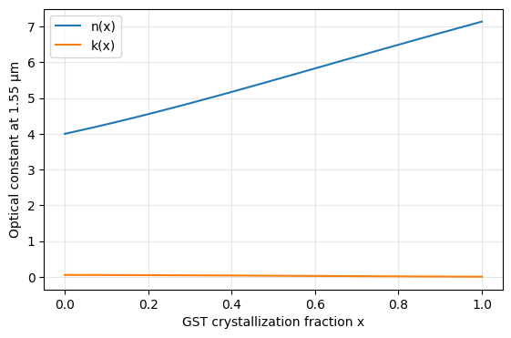
4. Bruggeman effective-medium model¶

Intermediate crystallization states use a symmetric Bruggeman mixture,

$ (1-x)\frac{\varepsilon_a-\varepsilon_{\rm eff}} {\varepsilon_a+2\varepsilon_{\rm eff}} + x\frac{\varepsilon_c-\varepsilon_{\rm eff}} {\varepsilon_c+2\varepsilon_{\rm eff}}=0, $

where (x=0) is amorphous and (x=1) is crystalline.

[4]:

def bruggeman_eps(x, eps_a, eps_c):
    x = np.asarray(x, dtype=float)
    B = 2 * eps_a - eps_c + 3 * x * (eps_c - eps_a)
    return (B + np.sqrt(B**2 + 8 * eps_a * eps_c)) / 4

def nk_from_eps(eps):
    n_complex = np.sqrt(eps)
    n_complex = np.where(np.real(n_complex) < 0, -n_complex, n_complex)
    return np.real(n_complex), np.abs(np.imag(n_complex))

eps_a = (N_A + 1j * K_A) ** 2
eps_c = (N_C + 1j * K_C) ** 2

x_dense = np.linspace(0, 1, 101)
eps_dense = bruggeman_eps(x_dense, eps_a, eps_c)
n_dense, k_dense = nk_from_eps(eps_dense)

plt.figure(figsize=(6.5, 4))
plt.plot(x_dense, n_dense, label="n(x)")
plt.plot(x_dense, k_dense, label="k(x)")
plt.xlabel("GST crystallization fraction x")
plt.ylabel("Optical constant at 1.55 µm")
plt.grid(alpha=0.3)
plt.legend()
plt.show()

def gst_medium_from_x(x):
    eps_eff = bruggeman_eps(float(x), eps_a, eps_c)
    n_eff, k_eff = nk_from_eps(np.array([eps_eff]))
    return td.Medium.from_nk(
        n=float(n_eff[0]), k=float(k_eff[0]), freq=freq0,
        name=f"GST_x_{x:.3f}"
    )

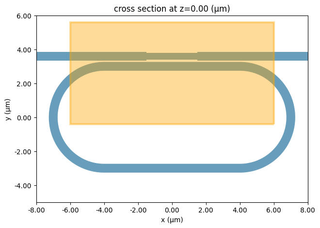
5. Racetrack and bus geometry¶

[5]:

def stadium_geometry(radius, straight, z0, height):
    rect = td.Box(center=(0, 0, z0), size=(straight, 2 * radius, height))
    left = td.Cylinder(
        center=(-straight / 2, 0, z0), axis=2,
        radius=radius, length=height
    )
    right = td.Cylinder(
        center=(straight / 2, 0, z0), axis=2,
        radius=radius, length=height
    )
    return (rect + left) + right

def racetrack_geometry(radius=R, width=wg_width,
                       straight=straight_length, z0=0.0,
                       height=wg_thickness):
    outer = stadium_geometry(radius + width / 2, straight, z0, height)
    inner = stadium_geometry(radius - width / 2, straight, z0, 1.5 * height)
    return outer - inner

def bus_geometry():
    total_length = 30.0
    center_length = 2 * Lcpl_half
    side_length = (total_length - center_length) / 2

    left = td.Box(
        center=(-(center_length + side_length) / 2, bus_y, 0),
        size=(side_length, wg_width, wg_thickness)
    )
    center = td.Box(
        center=(0, bus_y, 0),
        size=(center_length, coupler_width, wg_thickness)
    )
    right = td.Box(
        center=((center_length + side_length) / 2, bus_y, 0),
        size=(side_length, wg_width, wg_thickness)
    )
    return (left + center) + right

def gst_geometry():
    return td.Box(
        center=(0, R, wg_thickness / 2 + gst_thickness / 2),
        size=(gst_length, wg_width, gst_thickness)
    )

def spacer_geometry():
    z = wg_thickness / 2 + gst_thickness + spacer_thickness / 2
    return td.Box(
        center=(0, R, z),
        size=(heater_length, heater_width, spacer_thickness)
    )

def heater_geometry():
    z = wg_thickness / 2 + gst_thickness + spacer_thickness + ito_thickness / 2
    return td.Box(
        center=(0, R, z),
        size=(heater_length, heater_width, ito_thickness)
    )

6. Reusable 3D FDTD model¶

A fundamental bus-waveguide mode is launched from the left. Flux monitors measure input and through power, and an optional field monitor records the coupling region at 1.55 µm.

[6]:

def build_simulation(
    x_gst=0.0,
    include_gst=True,
    include_heater=False,
    include_racetrack=True,
    field_monitor=True,
):
    structures = [
        td.Structure(geometry=bus_geometry(), medium=Si, name="bus")
    ]

    if include_racetrack:
        structures.append(
            td.Structure(
                geometry=racetrack_geometry(),
                medium=Si,
                name="racetrack"
            )
        )

    if include_gst:
        structures.append(
            td.Structure(
                geometry=gst_geometry(),
                medium=gst_medium_from_x(x_gst),
                name="GST"
            )
        )

    if include_heater:
        structures += [
            td.Structure(
                geometry=spacer_geometry(),
                medium=SiO2,
                name="heater_spacer"
            ),
            td.Structure(
                geometry=heater_geometry(),
                medium=ITO,
                name="ITO_heater"
            ),
        ]

    source = td.ModeSource(
        center=(-13.0, bus_y, 0),
        size=(0, 2.5, 2.0),
        source_time=td.GaussianPulse(freq0=freq0, fwidth=fwidth),
        direction="+",
        mode_spec=td.ModeSpec(num_modes=1),
        mode_index=0,
        name="mode_source",
    )

    monitors = [
        td.FluxMonitor(
            center=(-10.5, bus_y, 0),
            size=(0, 2.5, 2.0),
            freqs=freqs,
            name="flux_in",
        ),
        td.FluxMonitor(
            center=(10.5, bus_y, 0),
            size=(0, 2.5, 2.0),
            freqs=freqs,
            name="flux_out",
        ),
    ]

    if field_monitor:
        monitors.append(
            td.FieldMonitor(
                center=(0, bus_y - 1.0, 0),
                size=(12.0, 6.0, 0),
                freqs=[freq0],
                fields=["Ex", "Ey", "Ez"],
                name="field_coupling",
            )
        )

    return td.Simulation(
        center=(0, 0.5, 0),
        size=sim_size,
        medium=SiO2,
        grid_spec=td.GridSpec.auto(
            wavelength=lambda0,
            min_steps_per_wvl=15
        ),
        structures=structures,
        sources=[source],
        monitors=monitors,
        run_time=run_time,
        boundary_spec=td.BoundarySpec.all_sides(
            boundary=td.PML()
        ),
        shutoff=1e-7,
    )

sim_preview = build_simulation(
    x_gst=0.0,
    include_heater=True
)

fig, ax = plt.subplots(figsize=(9, 5))
sim_preview.plot(z=0, ax=ax)
ax.set_xlim(-8, 8)
ax.set_ylim(-5, 6)
plt.show()

Mesh inspection¶

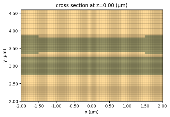
Because the GST, spacer, and heater are thin layers, inspect the local grid before launching publication-quality runs. If necessary, add a local mesh override or layer refinement.

[7]:

fig, ax = plt.subplots(figsize=(9, 4))
sim_preview.plot(z=0, ax=ax)
sim_preview.plot_grid(z=0, ax=ax)
ax.set_xlim(-2, 2)
ax.set_ylim(R - 1.0, bus_y + 1.0)
plt.show()

7. Optional endpoint cloud simulations¶

[8]:

def run_named(sim, task_name):
    path = DATA_DIR / f"{task_name}.hdf5"
    return web.run(
        sim,
        task_name=task_name,
        path=str(path),
        verbose=True
    )

endpoint_data = {}

if RUN_CLOUD:
    sims = {
        "aGST": build_simulation(
            x_gst=0.0,
            include_heater=False
        ),
        "cGST": build_simulation(
            x_gst=1.0,
            include_heater=False
        ),
        "bus_only": build_simulation(
            include_gst=False,
            include_heater=False,
            include_racetrack=False,
            field_monitor=False
        ),
    }

    for name, sim in sims.items():
        endpoint_data[name] = run_named(
            sim,
            f"gst_racetrack_{name}"
        )
else:
    print("RUN_CLOUD=False: no FlexCredits consumed.")

02:23:24 EDT Created task 'gst_racetrack_aGST' with resource_id                 
             'fdve-b3ea0fa5-2369-4d89-84c0-b397548d86ee' and task_type 'FDTD'.

             View task using web UI at                                          
             'https://tidy3d.simulation.cloud/workbench?taskId=fdve-b3ea0fa5-236
             9-4d89-84c0-b397548d86ee'.

             Task folder: 'default'.

Output()

02:23:26 EDT Estimated FlexCredit cost: 23.640. This assumes the FDTD solver    
             runs for the full simulation time; if early shutoff is reached, the
             billed cost can be lower. Use 'web.real_cost(task_id)' to get the  
             billed FlexCredit cost after a simulation run.

             status = success

Output()

02:23:28 EDT Loading results from data_gst_racetrack/gst_racetrack_aGST.hdf5

             Created task 'gst_racetrack_cGST' with resource_id                 
             'fdve-65db52bd-4d04-4fac-b319-213d23d7e51e' and task_type 'FDTD'.

             View task using web UI at                                          
             'https://tidy3d.simulation.cloud/workbench?taskId=fdve-65db52bd-4d0
             4-4fac-b319-213d23d7e51e'.

             Task folder: 'default'.

Output()

02:23:29 EDT Estimated FlexCredit cost: 37.804. This assumes the FDTD solver    
             runs for the full simulation time; if early shutoff is reached, the
             billed cost can be lower. Use 'web.real_cost(task_id)' to get the  
             billed FlexCredit cost after a simulation run.

02:23:30 EDT status = success

Output()

02:23:32 EDT Loading results from data_gst_racetrack/gst_racetrack_cGST.hdf5

             Created task 'gst_racetrack_bus_only' with resource_id             
             'fdve-5771a46e-73e5-4f2d-9c32-f6133461ceea' and task_type 'FDTD'.

             View task using web UI at                                          
             'https://tidy3d.simulation.cloud/workbench?taskId=fdve-5771a46e-73e
             5-4f2d-9c32-f6133461ceea'.

             Task folder: 'default'.

Output()

02:23:33 EDT Estimated FlexCredit cost: 15.797. This assumes the FDTD solver    
             runs for the full simulation time; if early shutoff is reached, the
             billed cost can be lower. Use 'web.real_cost(task_id)' to get the  
             billed FlexCredit cost after a simulation run.

02:23:34 EDT status = success

Output()

02:23:35 EDT Loading results from data_gst_racetrack/gst_racetrack_bus_only.hdf5

[9]:

def transmission_from_data(sim_data):
    pin = np.abs(
        np.asarray(
            sim_data["flux_in"].flux.values,
            dtype=float
        )
    )
    pout = np.abs(
        np.asarray(
            sim_data["flux_out"].flux.values,
            dtype=float
        )
    )
    return pout / pin

if endpoint_data:
    wl = td.C_0 / freqs
    order = np.argsort(wl)

    T_bus = transmission_from_data(
        endpoint_data["bus_only"]
    )
    T_a = transmission_from_data(
        endpoint_data["aGST"]
    ) / T_bus
    T_c = transmission_from_data(
        endpoint_data["cGST"]
    ) / T_bus

    plt.figure(figsize=(7, 4))
    plt.plot(wl[order], T_a[order], label="aGST")
    plt.plot(wl[order], T_c[order], label="cGST")
    plt.axvline(lambda0, ls="--", c="k", alpha=0.6)
    plt.xlabel("Wavelength (µm)")
    plt.ylabel("Bus-normalized transmission")
    plt.grid(alpha=0.3)
    plt.legend()
    plt.show()

8. Completed geometry-optimization result¶

The staged project search over gap, GST length, and coupling half-length produced:

$g=0.14~\mu\mathrm m$
$L_{\rm GST}=0.30~\mu\mathrm m$
$L_{\rm cpl}/2=1.50~\mu\mathrm m$
$T_{\rm aGST}=0.8866$
$T_{\rm cGST}=0.0707$
contrast $=0.8158$
extinction ratio $=10.98$ dB

The result is shown directly rather than automatically rerunning the expensive 3D geometry scan.

[10]:

optimization_summary = pd.DataFrame({
    "parameter": [
        "gap (µm)",
        "GST length (µm)",
        "Lcpl/2 (µm)",
        "T(aGST)",
        "T(cGST)",
        "contrast",
        "ER (dB)",
    ],
    "value": [
        0.14, 0.30, 1.50,
        0.8866, 0.0707,
        0.8158, 10.98
    ],
})
optimization_summary

[10]:

	parameter	value
0	gap (µm)	0.1400
1	GST length (µm)	0.3000
2	Lcpl/2 (µm)	1.5000
3	T(aGST)	0.8866
4	T(cGST)	0.0707
5	contrast	0.8158
6	ER (dB)	10.9800

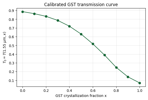
9. Dense GST calibration¶

Eleven crystallization states were simulated in the completed study. The values below reproduce the calibrated operating-point curve $T_0(x)=T(1.55~\mu\mathrm m,x)$ without consuming FlexCredits.

[11]:

x_report = np.linspace(0, 1, 11)
T0_report = np.array([
    0.8866,
    0.8635,
    0.8329,
    0.7866,
    0.7200,
    0.6301,
    0.5177,
    0.3899,
    0.2484,
    0.1399,
    0.0707,
])

eps_report = bruggeman_eps(
    x_report,
    eps_a,
    eps_c
)
n_report, k_report = nk_from_eps(eps_report)

calibration = pd.DataFrame({
    "x": x_report,
    "n_EMT": n_report,
    "k_EMT": k_report,
    "T0_1p55um": T0_report,
})
calibration

[11]:

	x	n_EMT	k_EMT	T0_1p55um
0	0.0	4.000000	5.000000e-02	0.8866
1	0.1	4.264388	4.728651e-02	0.8635
2	0.2	4.550143	4.349734e-02	0.8329
3	0.3	4.854019	3.876070e-02	0.7866
4	0.4	5.171728	3.332488e-02	0.7200
5	0.5	5.498585	2.749264e-02	0.6301
6	0.6	5.830135	2.154926e-02	0.5177
7	0.7	6.162591	1.571604e-02	0.3899
8	0.8	6.493013	1.013708e-02	0.2484
9	0.9	6.819287	4.889113e-03	0.1399
10	1.0	7.140000	9.718339e-19	0.0707

[12]:

plt.figure(figsize=(6.5, 4))
plt.plot(x_report, T0_report, "o-")
plt.xlabel("GST crystallization fraction x")
plt.ylabel(r"$T_0=T(1.55~\mu m,x)$")
plt.title("Calibrated GST transmission curve")
plt.grid(alpha=0.3)
plt.show()

Optional reproduction of the 11-state cloud sweep¶

[14]:

dense_data = {}

if RUN_DENSE_GST_SWEEP:
    for x_state in x_report:
        sim = build_simulation(
            x_gst=float(x_state),
            include_heater=False,
            field_monitor=False
        )
        task_name = (
            f"gst_x_{x_state:.2f}"
            .replace(".", "p")
        )
        dense_data[float(x_state)] = run_named(
            sim,
            task_name
        )
else:
    print("Dense GST sweep skipped.")

14:48:45 EDT Created task 'gst_x_0p00' with resource_id                         
             'fdve-2f34881a-6c23-4f5d-97c8-50b9133e6d53' and task_type 'FDTD'.

             View task using web UI at                                          
             'https://tidy3d.simulation.cloud/workbench?taskId=fdve-2f34881a-6c2
             3-4f5d-97c8-50b9133e6d53'.

             Task folder: 'default'.

Output()

14:48:47 EDT Estimated FlexCredit cost: 23.639. This assumes the FDTD solver    
             runs for the full simulation time; if early shutoff is reached, the
             billed cost can be lower. Use 'web.real_cost(task_id)' to get the  
             billed FlexCredit cost after a simulation run.

14:48:48 EDT status = success

Output()

14:48:49 EDT Loading results from data_gst_racetrack/gst_x_0p00.hdf5

             Created task 'gst_x_0p10' with resource_id                         
             'fdve-e0495baf-dd3a-43f9-9fe9-3fa352bffa64' and task_type 'FDTD'.

             View task using web UI at                                          
             'https://tidy3d.simulation.cloud/workbench?taskId=fdve-e0495baf-dd3
             a-43f9-9fe9-3fa352bffa64'.

             Task folder: 'default'.

Output()

14:48:51 EDT Estimated FlexCredit cost: 28.604. This assumes the FDTD solver    
             runs for the full simulation time; if early shutoff is reached, the
             billed cost can be lower. Use 'web.real_cost(task_id)' to get the  
             billed FlexCredit cost after a simulation run.

14:48:52 EDT status = success

Output()

14:48:53 EDT Loading results from data_gst_racetrack/gst_x_0p10.hdf5

             Created task 'gst_x_0p20' with resource_id                         
             'fdve-b53d4544-3dc3-4c7f-92ea-db9fbae3a8a9' and task_type 'FDTD'.

             View task using web UI at                                          
             'https://tidy3d.simulation.cloud/workbench?taskId=fdve-b53d4544-3dc
             3-4c7f-92ea-db9fbae3a8a9'.

             Task folder: 'default'.

Output()

14:48:55 EDT Estimated FlexCredit cost: 29.172. This assumes the FDTD solver    
             runs for the full simulation time; if early shutoff is reached, the
             billed cost can be lower. Use 'web.real_cost(task_id)' to get the  
             billed FlexCredit cost after a simulation run.

14:48:56 EDT status = success

Output()

             Loading results from data_gst_racetrack/gst_x_0p20.hdf5

14:48:57 EDT Created task 'gst_x_0p30' with resource_id                         
             'fdve-a779daa5-041f-4a6f-8201-3b62be3a1aed' and task_type 'FDTD'.

             View task using web UI at                                          
             'https://tidy3d.simulation.cloud/workbench?taskId=fdve-a779daa5-041
             f-4a6f-8201-3b62be3a1aed'.

             Task folder: 'default'.

Output()

14:48:58 EDT Estimated FlexCredit cost: 29.188. This assumes the FDTD solver    
             runs for the full simulation time; if early shutoff is reached, the
             billed cost can be lower. Use 'web.real_cost(task_id)' to get the  
             billed FlexCredit cost after a simulation run.

14:48:59 EDT status = success

Output()

14:49:00 EDT Loading results from data_gst_racetrack/gst_x_0p30.hdf5

14:49:01 EDT Created task 'gst_x_0p40' with resource_id                         
             'fdve-19ea40db-285b-44f9-9b42-04786a607436' and task_type 'FDTD'.

             View task using web UI at                                          
             'https://tidy3d.simulation.cloud/workbench?taskId=fdve-19ea40db-285
             b-44f9-9b42-04786a607436'.

             Task folder: 'default'.

Output()

14:49:02 EDT Estimated FlexCredit cost: 30.821. This assumes the FDTD solver    
             runs for the full simulation time; if early shutoff is reached, the
             billed cost can be lower. Use 'web.real_cost(task_id)' to get the  
             billed FlexCredit cost after a simulation run.

14:49:03 EDT status = success

Output()

14:49:04 EDT Loading results from data_gst_racetrack/gst_x_0p40.hdf5

             Created task 'gst_x_0p50' with resource_id                         
             'fdve-7cd1d6c0-3876-4480-ac14-518c9085b07b' and task_type 'FDTD'.

             View task using web UI at                                          
             'https://tidy3d.simulation.cloud/workbench?taskId=fdve-7cd1d6c0-387
             6-4480-ac14-518c9085b07b'.

             Task folder: 'default'.

Output()

14:49:06 EDT Estimated FlexCredit cost: 30.866. This assumes the FDTD solver    
             runs for the full simulation time; if early shutoff is reached, the
             billed cost can be lower. Use 'web.real_cost(task_id)' to get the  
             billed FlexCredit cost after a simulation run.

14:49:07 EDT status = success

Output()

14:49:08 EDT Loading results from data_gst_racetrack/gst_x_0p50.hdf5

             Created task 'gst_x_0p60' with resource_id                         
             'fdve-77bdfc6b-cea9-44d0-b1c3-14aa791b3e20' and task_type 'FDTD'.

             View task using web UI at                                          
             'https://tidy3d.simulation.cloud/workbench?taskId=fdve-77bdfc6b-cea
             9-44d0-b1c3-14aa791b3e20'.

             Task folder: 'default'.

Output()

14:49:10 EDT Estimated FlexCredit cost: 31.337. This assumes the FDTD solver    
             runs for the full simulation time; if early shutoff is reached, the
             billed cost can be lower. Use 'web.real_cost(task_id)' to get the  
             billed FlexCredit cost after a simulation run.

14:49:11 EDT status = success

Output()

14:49:12 EDT Loading results from data_gst_racetrack/gst_x_0p60.hdf5

             Created task 'gst_x_0p70' with resource_id                         
             'fdve-f991a99b-d95a-4d34-bfa6-bde20f185551' and task_type 'FDTD'.

             View task using web UI at                                          
             'https://tidy3d.simulation.cloud/workbench?taskId=fdve-f991a99b-d95
             a-4d34-bfa6-bde20f185551'.

             Task folder: 'default'.

Output()

14:49:14 EDT Estimated FlexCredit cost: 32.724. This assumes the FDTD solver    
             runs for the full simulation time; if early shutoff is reached, the
             billed cost can be lower. Use 'web.real_cost(task_id)' to get the  
             billed FlexCredit cost after a simulation run.

14:49:15 EDT status = queued

             To cancel the simulation, use 'web.abort(task_id)' or              
             'web.delete(task_id)' or abort/delete the task in the web UI.      
             Terminating the Python script will not stop the job running on the 
             cloud.

Output()

14:49:30 EDT starting up solver

             running solver

Output()

14:52:51 EDT early shutoff detected at 0%, exiting.

14:52:52 EDT status = queued

Output()

14:53:02 EDT status = preprocess

14:53:04 EDT status = running

15:38:48 EDT status = success

15:38:50 EDT View simulation result at                                          
             'https://tidy3d.simulation.cloud/workbench?taskId=fdve-f991a99b-d95
             a-4d34-bfa6-bde20f185551'.

Output()

15:38:51 EDT Loading results from data_gst_racetrack/gst_x_0p70.hdf5

             Created task 'gst_x_0p80' with resource_id                         
             'fdve-a0be140e-ee05-4831-ab58-64c0700cc346' and task_type 'FDTD'.

             View task using web UI at                                          
             'https://tidy3d.simulation.cloud/workbench?taskId=fdve-a0be140e-ee0
             5-4831-ab58-64c0700cc346'.

             Task folder: 'default'.

Output()

15:38:53 EDT Estimated FlexCredit cost: 35.448. This assumes the FDTD solver    
             runs for the full simulation time; if early shutoff is reached, the
             billed cost can be lower. Use 'web.real_cost(task_id)' to get the  
             billed FlexCredit cost after a simulation run.

15:38:54 EDT status = queued

             To cancel the simulation, use 'web.abort(task_id)' or              
             'web.delete(task_id)' or abort/delete the task in the web UI.      
             Terminating the Python script will not stop the job running on the 
             cloud.

Output()

15:39:09 EDT starting up solver

             running solver

Output()

15:49:57 EDT early shutoff detected at 1%, exiting.

             status = queued

Output()

15:50:48 EDT status = running

18:18:35 EDT status = queued

18:18:47 EDT status = preprocess

18:18:49 EDT status = running

20:02:48 EDT status = success

20:02:50 EDT View simulation result at                                          
             'https://tidy3d.simulation.cloud/workbench?taskId=fdve-a0be140e-ee0
             5-4831-ab58-64c0700cc346'.

Output()

20:02:51 EDT Loading results from data_gst_racetrack/gst_x_0p80.hdf5

             Created task 'gst_x_0p90' with resource_id                         
             'fdve-2b625d69-e4c2-47fe-ad25-5712f059735f' and task_type 'FDTD'.

             View task using web UI at                                          
             'https://tidy3d.simulation.cloud/workbench?taskId=fdve-2b625d69-e4c
             2-47fe-ad25-5712f059735f'.

             Task folder: 'default'.

Output()

20:02:53 EDT Estimated FlexCredit cost: 37.410. This assumes the FDTD solver    
             runs for the full simulation time; if early shutoff is reached, the
             billed cost can be lower. Use 'web.real_cost(task_id)' to get the  
             billed FlexCredit cost after a simulation run.

20:02:54 EDT status = queued

             To cancel the simulation, use 'web.abort(task_id)' or              
             'web.delete(task_id)' or abort/delete the task in the web UI.      
             Terminating the Python script will not stop the job running on the 
             cloud.

Output()

20:03:08 EDT starting up solver

20:03:09 EDT running solver

Output()

20:14:08 EDT early shutoff detected at 1%, exiting.

             status = queued

Output()

20:14:58 EDT status = preprocess

20:15:01 EDT status = running

22:07:46 EDT status = postprocess

22:07:49 EDT status = success

22:07:51 EDT View simulation result at                                          
             'https://tidy3d.simulation.cloud/workbench?taskId=fdve-2b625d69-e4c
             2-47fe-ad25-5712f059735f'.

Output()

22:07:52 EDT Loading results from data_gst_racetrack/gst_x_0p90.hdf5

             Created task 'gst_x_1p00' with resource_id                         
             'fdve-200bea1e-d00f-4ab5-818c-8bb1bc5dab1a' and task_type 'FDTD'.

             View task using web UI at                                          
             'https://tidy3d.simulation.cloud/workbench?taskId=fdve-200bea1e-d00
             f-4ab5-818c-8bb1bc5dab1a'.

             Task folder: 'default'.

Output()

22:07:54 EDT Estimated FlexCredit cost: 37.803. This assumes the FDTD solver    
             runs for the full simulation time; if early shutoff is reached, the
             billed cost can be lower. Use 'web.real_cost(task_id)' to get the  
             billed FlexCredit cost after a simulation run.

22:07:55 EDT status = queued

             To cancel the simulation, use 'web.abort(task_id)' or              
             'web.delete(task_id)' or abort/delete the task in the web UI.      
             Terminating the Python script will not stop the job running on the 
             cloud.

Output()

22:08:05 EDT status = preprocess

22:08:09 EDT starting up solver

22:08:10 EDT running solver

Output()

22:08:30 EDT early shutoff detected at 0%, exiting.

             status = queued

Output()

22:08:52 EDT status = preprocess

22:08:54 EDT status = running

22:10:15 EDT status = queued

22:10:38 EDT status = preprocess

22:10:41 EDT status = running

23:03:24 EDT status = postprocess

23:03:26 EDT status = success

23:03:28 EDT View simulation result at                                          
             'https://tidy3d.simulation.cloud/workbench?taskId=fdve-200bea1e-d00
             f-4ab5-818c-8bb1bc5dab1a'.

Output()

23:03:29 EDT Loading results from data_gst_racetrack/gst_x_1p00.hdf5

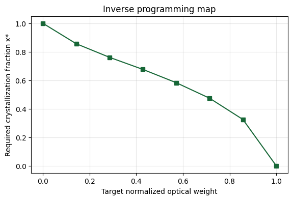
10. Inverse programming map¶

Define

$ W_{\rm opt}= \frac{T_0-T_{\min}} {T_{\max}-T_{\min}}. $

For target $W^*$,

$ T^*= T_{\min}+W^*(T_{\max}-T_{\min}), $

and the monotonic calibration curve is inverted to obtain the required crystallization state $x^*$.

[15]:

Tmin = float(T0_report.min())
Tmax = float(T0_report.max())

def x_from_target_T(T_target):
    return float(
        np.interp(
            T_target,
            T0_report[::-1],
            x_report[::-1]
        )
    )

W8 = np.linspace(0, 1, 8)
T8_target = Tmin + W8 * (Tmax - Tmin)
x8 = np.array([
    x_from_target_T(T)
    for T in T8_target
])

inverse_map = pd.DataFrame({
    "level": np.arange(8),
    "W_target": W8,
    "T_target": T8_target,
    "x_required": x8,
})
inverse_map

[15]:

	level	W_target	T_target	x_required
0	0	0.000000	0.070700	1.000000
1	1	0.142857	0.187257	0.856353
2	2	0.285714	0.303814	0.760838
3	3	0.428571	0.420371	0.676157
4	4	0.571429	0.536929	0.582893
5	5	0.714286	0.653486	0.473987
6	6	0.857143	0.770043	0.324861
7	7	1.000000	0.886600	0.000000

[16]:

plt.figure(figsize=(6.5, 4))
plt.plot(W8, x8, "s-")
plt.xlabel("Target normalized optical weight")
plt.ylabel("Required crystallization fraction x*")
plt.title("Inverse programming map")
plt.grid(alpha=0.3)
plt.show()

11. Optical multiplication¶

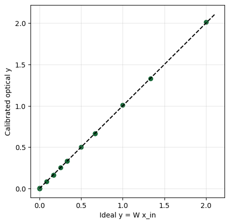
For each fixed GST state,

$ P_{\rm out}=T\,P_{\rm in}. $

After affine calibration, the normalized transmission represents a scalar optical weight. The completed project reported $R^2=0.99998$ for the scalar multiplication study.

[17]:

W4 = np.array([0.0, 1/3, 2/3, 1.0])

T4_achieved = np.array([
    0.0725,
    0.3425,
    0.6145,
    0.8927
])

W4_achieved = (
    (T4_achieved - Tmin)
    / (Tmax - Tmin)
)

x_inputs = np.array([
    0.25, 0.50, 1.0, 2.0
])

y_ideal = np.outer(
    x_inputs,
    W4
).ravel()

y_model = np.outer(
    x_inputs,
    W4_achieved
).ravel()

mae = np.mean(
    np.abs(y_model - y_ideal)
)
rmse = np.sqrt(
    np.mean((y_model - y_ideal) ** 2)
)
r2 = 1 - (
    np.sum((y_model - y_ideal) ** 2)
    / np.sum((y_ideal - y_ideal.mean()) ** 2)
)

print(f"MAE  = {mae:.4e}")
print(f"RMSE = {rmse:.4e}")
print(f"R^2  = {r2:.8f}")

plt.figure(figsize=(5, 5))
plt.scatter(y_ideal, y_model)
lim = max(y_ideal.max(), y_model.max()) * 1.05
plt.plot([0, lim], [0, lim], "k--")
plt.xlabel("Ideal y = W x_in")
plt.ylabel("Calibrated optical y")
plt.grid(alpha=0.3)
plt.show()

MAE  = 2.3555e-03
RMSE = 4.4942e-03
R^2  = 0.99993194

Extended write path¶

The remaining simulation chain is

$ W^* \rightarrow V(t) \rightarrow T_{\rm GST}(t) \rightarrow x \rightarrow n(x),k(x) \rightarrow T_{\rm optical}. $

The following thermal/kinetic cells are explicitly labeled as surrogate design exploration.

12. ITO-heater optical penalty¶

An ITO heater is placed above the GST with a 50-nm silica spacer. The completed optical study found:

contrast without heater: 0.8158
contrast with heater: 0.8202
reported aGST $\Delta IL$: $-0.03$ dB

The small negative sign should not be interpreted as optical gain; in a resonant structure the added layer can shift the operating point slightly. The useful conclusion is that the modeled heater caused a small optical perturbation.

[18]:

heater_optical_summary = pd.DataFrame({
    "metric": [
        "contrast without heater",
        "contrast with heater",
        "reported ΔIL(aGST) [dB]",
    ],
    "value": [
        0.8158,
        0.8202,
        -0.0300
    ],
})
heater_optical_summary

[18]:

	metric	value
0	contrast without heater	0.8158
1	contrast with heater	0.8202
2	reported ΔIL(aGST) [dB]	-0.0300

13. Lumped electrothermal model¶

The exploratory thermal model is

$$ C_{\rm th}\frac{dT}{dt} = \frac{V^2}{R_{\rm heater}} - \frac{T-T_{\rm amb}}{R_{\rm th}}. $$

The project used $R_{\rm th}=8\times10^4$ K/W and $C_{\rm th}=2\times10^{-12}$ J/K. The effective heater resistance below is calibrated from the reported SET candidate so that no hidden resistance value is invented.

[19]:

R_th = 8.0e4
C_th = 2.0e-12
T_amb_C = 25.0

V_set_ref = 0.420
tau_set_ref = 2.60e-6
T_set_ref_C = 366.0

tau_th = R_th * C_th
frac = 1 - np.exp(
    -tau_set_ref / tau_th
)

R_heater = (
    V_set_ref**2
    * R_th
    * frac
    / (T_set_ref_C - T_amb_C)
)

print(
    f"Thermal time constant = "
    f"{tau_th*1e6:.3f} µs"
)
print(
    f"Calibrated effective "
    f"R_heater ≈ {R_heater:.2f} Ω"
)

def thermal_trace(
    V,
    pulse_width,
    t_end=None,
    dt=None
):
    if t_end is None:
        t_end = (
            pulse_width
            + max(
                10 * tau_th,
                0.5 * pulse_width
            )
        )

    if dt is None:
        dt = min(
            max(
                pulse_width / 500,
                1e-10
            ),
            tau_th / 50
        )

    t = np.arange(
        0,
        t_end + dt,
        dt
    )

    delta_ss = (
        V**2 / R_heater
    ) * R_th

    T_end = (
        T_amb_C
        + delta_ss
        * (
            1
            - np.exp(
                -pulse_width
                / tau_th
            )
        )
    )

    T = np.empty_like(t)
    on = t <= pulse_width

    T[on] = (
        T_amb_C
        + delta_ss
        * (
            1
            - np.exp(
                -t[on] / tau_th
            )
        )
    )

    off_t = (
        t[~on]
        - pulse_width
    )

    T[~on] = (
        T_amb_C
        + (T_end - T_amb_C)
        * np.exp(
            -off_t / tau_th
        )
    )

    return t, T

t_set, T_set = thermal_trace(
    0.420,
    2.60e-6
)

t_reset, T_reset = thermal_trace(
    1.200,
    50e-9,
    t_end=2.0e-6
)

plt.figure(figsize=(7, 4))
plt.plot(
    t_set * 1e6,
    T_set,
    label="SET-like candidate"
)
plt.plot(
    t_reset * 1e6,
    T_reset,
    label="RESET-like candidate"
)
plt.xlabel("Time (µs)")
plt.ylabel("Lumped temperature (°C)")
plt.grid(alpha=0.3)
plt.legend()
plt.show()

print(
    f"SET-like Tmax = "
    f"{T_set.max():.1f} °C"
)
print(
    f"RESET-like Tmax = "
    f"{T_reset.max():.1f} °C"
)

Thermal time constant = 0.160 µs
Calibrated effective R_heater ≈ 41.38 Ω

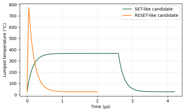
SET-like Tmax = 366.0 °C
RESET-like Tmax = 772.1 °C

14. GST crystallization kinetics¶

A JMAK-like reduced-time model converts thermal history to crystallization fraction:

$ K(T)=K_0\exp\left( -\frac{E_a}{k_B T} \right), \qquad x=1-\exp[-\Theta^m], \qquad \Theta=\int K(T)\,dt. $

The project surrogate used approximately $E_a=2.0$ eV and $K_0=5\times10^{21}\ {\rm s}^{-1}$. Replace these values with stack-specific measurements or a cited validated model before publication.

[20]:

kB_eV = 8.617333262e-5
Ea_eV = 2.0
K0 = 5.0e21
avrami_m = 2.0

T_cryst_C = 160.0
T_melt_C = 630.0

def jmak_from_temperature(
    t,
    T_C,
    x0=0.0
):
    T_K = T_C + 273.15
    dt = np.diff(
        t,
        prepend=t[0]
    )

    K = (
        K0
        * np.exp(
            -Ea_eV
            / (kB_eV * T_K)
        )
    )

    K = np.where(
        T_C >= T_cryst_C,
        K,
        0.0
    )

    theta = np.cumsum(
        K * dt
    )

    transformed = (
        1
        - np.exp(
            -(theta ** avrami_m)
        )
    )

    x = (
        x0
        + (1 - x0)
        * transformed
    )

    if np.max(T_C) >= T_melt_C:
        x[:] = 0.0

    return np.clip(
        x,
        0,
        1
    )

x_set_trace = jmak_from_temperature(
    t_set,
    T_set,
    x0=0.0
)

x_reset_trace = jmak_from_temperature(
    t_reset,
    T_reset,
    x0=1.0
)

plt.figure(figsize=(7, 4))
plt.plot(
    t_set * 1e6,
    x_set_trace,
    label="SET-like x(t)"
)
plt.plot(
    t_reset * 1e6,
    x_reset_trace,
    label="RESET-like x(t)"
)
plt.xlabel("Time (µs)")
plt.ylabel("Crystallization fraction x")
plt.ylim(-0.05, 1.05)
plt.grid(alpha=0.3)
plt.legend()
plt.show()

print(
    "SET-like final x =",
    x_set_trace[-1]
)
print(
    "RESET-like final x =",
    x_reset_trace[-1]
)

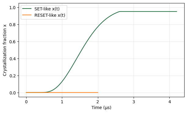
SET-like final x = 0.9496729146027164
RESET-like final x = 0.0

15. Dense surrogate pulse library¶

[21]:

voltages = np.linspace(
    0.34,
    0.42,
    13
)

durations_us = np.geomspace(
    1.0,
    500.0,
    14
)

pulse_rows = []

for V in voltages:
    for tau_us in durations_us:
        t, T = thermal_trace(
            V,
            tau_us * 1e-6
        )
        x_tr = jmak_from_temperature(
            t,
            T,
            x0=0.0
        )
        pulse_rows.append({
            "V": V,
            "tau_us": tau_us,
            "Tmax_C": float(T.max()),
            "x_final": float(
                x_tr[-1]
            ),
        })

pulse_library = pd.DataFrame(
    pulse_rows
)

plt.figure(figsize=(7, 5))
sc = plt.scatter(
    pulse_library["V"],
    pulse_library["tau_us"],
    c=pulse_library["x_final"],
    s=45
)
plt.yscale("log")
plt.xlabel("Pulse voltage (V)")
plt.ylabel("Pulse width (µs)")
plt.title(
    "Surrogate SET programming library"
)
plt.colorbar(
    sc,
    label="Final crystallization fraction x"
)
plt.show()

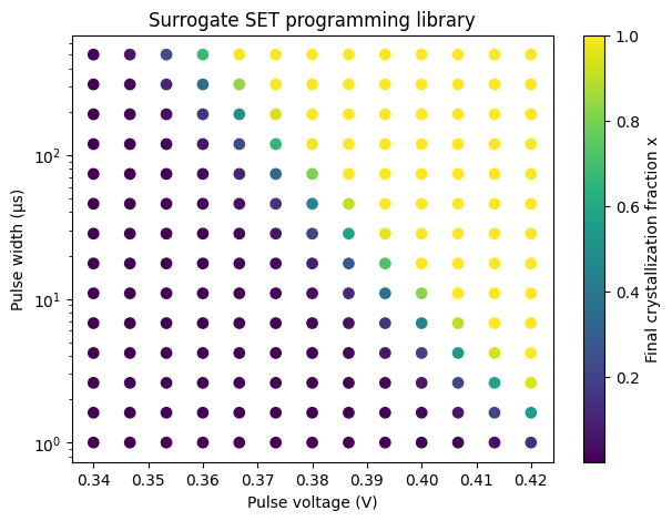
16. Four target optical levels¶

The robustness study intentionally reduced the nominal 8-level ladder to four states before making a multilevel claim:

$ W=\{0,\;1/3,\;2/3,\;1\}. $

[22]:

W4_target = np.array([
    0.0,
    1/3,
    2/3,
    1.0
])

T4_target = (
    Tmin
    + W4_target
    * (Tmax - Tmin)
)

x4_target = np.array([
    x_from_target_T(T)
    for T in T4_target
])

four_level_targets = pd.DataFrame({
    "level": np.arange(4),
    "W_target": W4_target,
    "T_target": T4_target,
    "x_target": x4_target,
})
four_level_targets

[22]:

	level	W_target	T_target	x_target
0	0	0.000000	0.070700	1.00000
1	1	0.333333	0.342667	0.73338
2	2	0.666667	0.614633	0.51376
3	3	1.000000	0.886600	0.00000

17. Simulated write-verify¶

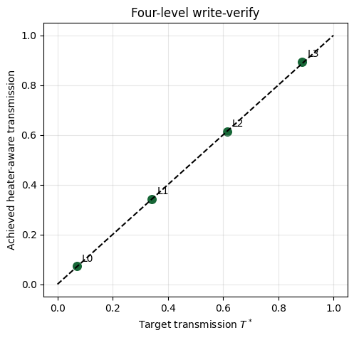
The completed heater-aware write-verify simulation converged all four target states within $\epsilon_T=0.02$:

$0.0707\rightarrow0.0725$
$0.3427\rightarrow0.3425$
$0.6146\rightarrow0.6145$
$0.8866\rightarrow0.8927$

The pulse values are literature-parameterized surrogates only.

[23]:

T4_completed = np.array([
    0.0725,
    0.3425,
    0.6145,
    0.8927
])

plt.figure(figsize=(5.5, 5.0))
plt.scatter(
    T4_target,
    T4_completed,
    s=70
)
plt.plot(
    [0, 1],
    [0, 1],
    "k--"
)

for i, (
    xt,
    ya
) in enumerate(
    zip(
        T4_target,
        T4_completed
    )
):
    plt.annotate(
        f"L{i}",
        (xt, ya),
        xytext=(5, 5),
        textcoords="offset points"
    )

plt.xlabel(
    "Target transmission $T^*$"
)
plt.ylabel(
    "Achieved heater-aware transmission"
)
plt.title(
    "Four-level write-verify"
)
plt.grid(alpha=0.3)
plt.show()

write_verify_table = pd.DataFrame({
    "level": np.arange(4),
    "T_target": T4_target,
    "T_achieved": T4_completed,
    "abs_error": np.abs(
        T4_completed
        - T4_target
    ),
})

write_verify_table

[23]:

	level	T_target	T_achieved	abs_error
0	0	0.070700	0.0725	0.001800
1	1	0.342667	0.3425	0.000167
2	2	0.614633	0.6145	0.000133
3	3	0.886600	0.8927	0.006100

18. Robust multilevel separation¶

The completed heater-aware uncertainty study found the best tested gap at $g=0.14~\mu\mathrm m$, with

$ M_{\rm worst}=0.1586>0. $

Thus the supported modeled robust level count is

$ N_{\rm robust}=4, \qquad b_{\rm eff}=\log_2(4)=2~\text{bits}. $

This should be reported separately from the nominal 8-level optical calibration.

[24]:

M_worst = 0.1586
N_robust = 4
b_eff = np.log2(
    N_robust
)

robust_summary = pd.DataFrame({
    "metric": [
        "best gap (µm)",
        "M_worst",
        "robust level count",
        "effective bit depth",
    ],
    "value": [
        0.14,
        M_worst,
        N_robust,
        b_eff,
    ],
})

robust_summary

[24]:

	metric	value
0	best gap (µm)	0.1400
1	M_worst	0.1586
2	robust level count	4.0000
3	effective bit depth	2.0000

19. Conclusions¶

This notebook demonstrates a Tidy3D-centered simulation workflow for a GST-programmable silicon racetrack:

optimized aGST/cGST contrast near 1.55 µm;
linear fixed-state optical readout;
Bruggeman intermediate-state calibration;
inverse mapping from target optical weight to GST state;
scalar optical multiplication;
heater-aware optical modeling;
a literature-parameterized pulse-to-crystallization surrogate;
four-level write-verify;
robustness-aware ~2-bit modeled operation.

All results shown here are simulation / literature-parameterized models suitable for community learning and design exploration within Tidy3D.

References and Tidy3D resources¶

Tidy3D documentation

Suggested scientific background

M. Wuttig, H. Bhaskaran, and T. Taubner, "Phase-change materials for non-volatile photonic applications," Nature Photonics 11, 465-476 (2017).
C. Rios et al., "Integrated all-photonic non-volatile multi-level memory," Nature Photonics 9, 725-732 (2015).
J. Feldmann et al., "Parallel convolutional processing using an integrated photonic tensor core," Nature 589, 52-58 (2021).
D. A. G. Bruggeman, "Berechnung verschiedener physikalischer Konstanten von heterogenen Substanzen," Ann. Phys. 416, 636-664 (1935).

[ ]:

TIDY3D
LEARNING CENTER

Programmable Multilevel Photonic Transmission Using a GST-Loaded Silicon Racetrack Resonator¶

1. Imports¶

2. Global parameters¶

3. Materials¶

4. Bruggeman effective-medium model¶

5. Racetrack and bus geometry¶

6. Reusable 3D FDTD model¶

Mesh inspection¶

7. Optional endpoint cloud simulations¶

8. Completed geometry-optimization result¶

9. Dense GST calibration¶

Optional reproduction of the 11-state cloud sweep¶

10. Inverse programming map¶

11. Optical multiplication¶

Extended write path¶

12. ITO-heater optical penalty¶

13. Lumped electrothermal model¶

14. GST crystallization kinetics¶

15. Dense surrogate pulse library¶

16. Four target optical levels¶

17. Simulated write-verify¶

18. Robust multilevel separation¶

19. Conclusions¶

References and Tidy3D resources¶

More Notebooks

TIDY3D LEARNING CENTER

Programmable Multilevel Photonic Transmission Using a GST-Loaded Silicon Racetrack Resonator¶

1. Imports¶

2. Global parameters¶

3. Materials¶

4. Bruggeman effective-medium model¶

5. Racetrack and bus geometry¶

6. Reusable 3D FDTD model¶

Mesh inspection¶

7. Optional endpoint cloud simulations¶

8. Completed geometry-optimization result¶

9. Dense GST calibration¶

Optional reproduction of the 11-state cloud sweep¶

10. Inverse programming map¶

11. Optical multiplication¶

Extended write path¶

12. ITO-heater optical penalty¶

13. Lumped electrothermal model¶

14. GST crystallization kinetics¶

15. Dense surrogate pulse library¶

16. Four target optical levels¶

17. Simulated write-verify¶

18. Robust multilevel separation¶

19. Conclusions¶

References and Tidy3D resources¶

More Notebooks

Cookie preferences

Privacy choices

TIDY3D
LEARNING CENTER