The Challenge: Differentiating Complex Simulations

Optimizing photonic devices often involves finding the best set of design parameters (e.g., taper shape) that maximize or minimize a specific outcome (e.g., coupling efficiency). Gradient-based optimization methods are highly effective for this, but they require knowing how sensitive the outcome is to small changes in each parameter.

Calculating this gradient for a complex FDTD simulation is challenging. A naive approach (like finite differences) would require running many simulations – one for each parameter – which quickly becomes computationally infeasible for designs with many variables.

Our Solution: Combining autograd and the Adjoint Method

Tidy3D leverages the autograd library for automatic differentiation. When you write a Python function that defines your simulation setup, runs tidy3d.web.run, and calculates a final figure of merit, autograd can automatically track all the mathematical operations outside the simulation.

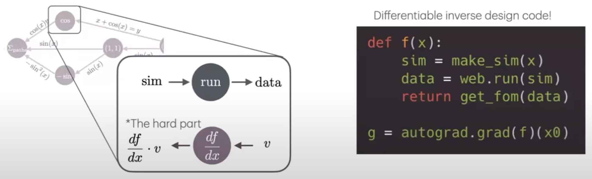
However, autograd doesn’t inherently know how to differentiate through the FDTD simulation node. This is where Tidy3D’s custom integration comes in, using the adjoint method.

We’ve essentially “taught” autograd the derivative rule for the tidy3d.web.run operation. This rule is implemented using the adjoint method, a powerful technique derived from electromagnetic theory.

Key Benefit of the Adjoint Method: It allows us to compute the gradient of the figure of merit with respect to all design parameters using just one additional simulation (the adjoint simulation), regardless of how many parameters there are (hundreds, thousands, or even millions).

The Differentiation Pipeline: Forward and Backward Passes

When you ask autograd to compute the gradient (e.g., using autograd.grad(objective_function)), here’s a simplified view of what happens under the hood:

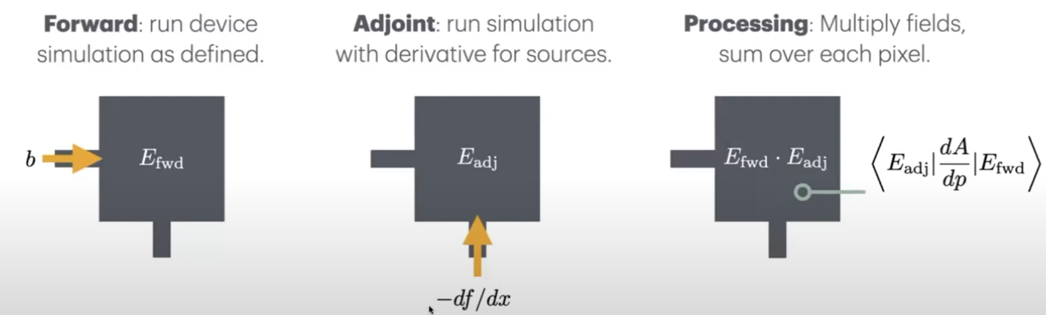
1. Forward Pass:
   • Your Python function executes normally.
   • Tidy3D components (td.Structure, td.Box, td.Medium, etc.) are created, potentially using autograd tracked numbers (from autograd.numpy).
   • tidy3d.web.run(simulation) is called. The standard forward FDTD simulation runs.
   • Crucially, during this forward run, Tidy3D automatically stores necessary field information in the regions relevant to the differentiable parameters (e.g., near the boundaries of a shape-optimized geometry).
   • The simulation results (SimulationData) are returned.
   • Your function calculates the final scalar objective value using autograd.numpy operations. autograd builds the computational graph along the way.
2. Backward Pass (Vector-Jacobian Product - VJP):
   • autograd starts propagating gradient information backward through the computational graph using the chain rule.
   • When it reaches the td.web.run node, Tidy3D’s custom VJP function takes over.
   • This function uses the gradient information flowing into it (representing the sensitivity of the final objective to the simulation’s outputs, like monitor data) to set up adjoint sources.
   • An adjoint FDTD simulation is automatically configured and run.
   • Tidy3D combines the stored fields from the forward simulation with the results of the adjoint simulation.
   • Using custom gradient rules, it efficiently calculates the partial derivative of the objective function with respect to every single tracked design parameter.
   • These parameter gradients are packaged and returned to autograd.
   • autograd continues the backward pass until it reaches the original input parameters, yielding the final overall gradient.

How Tidy3D Components Compute Gradients

Different types of parameters require different specific calculations within the adjoint method framework. Tidy3D handles this internally:

• Shape Optimization: For parameters defining geometry (e.g., Box.center, Box.size, PolySlab.vertices), gradients are typically computed using surface integrals involving the forward and adjoint fields on the boundaries of the shape. Moving a boundary slightly changes the permittivity locally, and the adjoint method quantifies the impact of this change on the objective.
• Material Optimization (Topology Optimization): For parameters defining material properties (e.g., the permittivity in each voxel of a CustomMedium), gradients are computed using the forward and adjoint fields within that material region.

You don’t need to worry about these formulas – Tidy3D components like td.Box, td.Cylinder, td.Medium, td.CustomMedium, etc., have their differentiation logic built-in.

The User Experience: Seamless Integration

The beauty of this approach is its simplicity from the user’s perspective:

1. Define your objective function in Python using standard Tidy3D components and autograd.numpy for numerical operations.
2. Call td.web.run() within your function as usual.
3. Use autograd.grad() (or related functions like value_and_grad) to get the gradient.

Tidy3D and autograd handle the complex forward simulation, field storage, adjoint simulation setup, adjoint run, and final gradient calculation automatically behind the scenes. You get the efficiency of the adjoint method without needing to implement it yourself.

Conclusion

Tidy3D’s integration with autograd via the adjoint method provides a powerful, flexible, and efficient platform for inverse design and sensitivity analysis. By defining a custom derivative rule for FDTD simulations, we unlock the ability to use gradient-based optimization on complex photonic design problems, requiring only one forward and one adjoint simulation per optimization step, regardless of the number of design parameters. This dramatically accelerates the design cycle for cutting-edge photonic devices.

Next Steps / Further Reading:

1. Topology optimization of a mode converter
2. Shape optimization of a waveguide bend
3. Level set optimization of a y-branch
4. Fabrication-aware inverse design