





from typing import List

import autograd.numpy as anp
import matplotlib.pylab as plt
import numpy as np

# import regular tidy3d
import tidy3d as td
import tidy3d.web as web
from autograd import value_and_grad
from tidy3d.plugins.mode import ModeSolver

# set random seed to get same results
np.random.seed(2)
TIDY3D
LEARNING CENTER
Example Library

Inverse design optimization of a mode converter
In this notebook, we will use inverse design and Tidy3D to create an integrated photonics component to convert a fundamental waveguide mode to a higher order mode.
Setup
We wish to recreate a device like the diagram below:
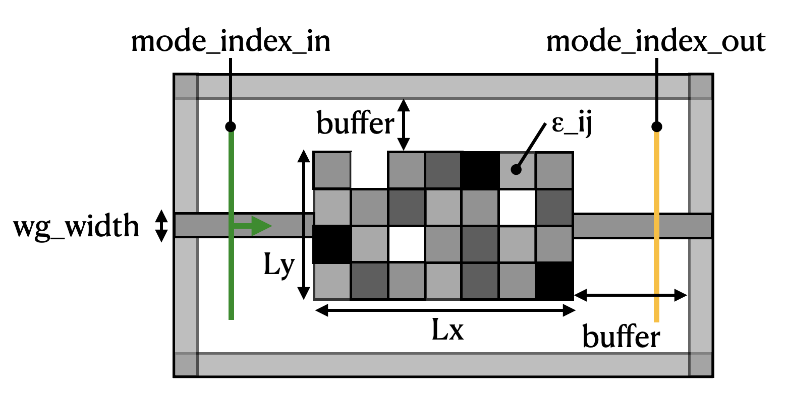
A mode source is injected into a waveguide on the left-hand side. The light propagates through a rectangular region with pixelated permittivity with the value of each pixel independently tunable between 1 (vacuum) and some maximum permittivity. Finally, we measure the transmission of the light into a waveguide on the right-hand side.
The goal of the inverse design exercise is to find the best distribution of permittivities (\(\epsilon_{ij}\)) in the coupling region to maximize the power conversion between the input mode and the output mode.
We also apply our built-in smoothening and binarization filters to ensure that the final device has smooth features, and permittivity values that are all either 1, or the maximum permittivity of the waveguide material.
Parameters
First we will define some parameters.
# wavelength and frequency
wavelength = 1.0
freq0 = td.C_0 / wavelength
k0 = 2 * np.pi * freq0 / td.C_0

# resolution control
min_steps_per_wvl = 16
# in the design region, we set uniform grid resolution,
# and define the design parameters on the same grid
dl_design_region = 0.01

# space between boxes and PML
buffer = 1.0 * wavelength

# optimize region size
lz = td.inf
lx = 5.0
ly = 3.0

# position of source and monitor (constant for all)
source_x = -lx / 2 - buffer * 0.8
meas_x = lx / 2 + buffer * 0.8

# total size
Lx = lx + 2 * buffer
Ly = ly + 2 * buffer
Lz = 0.0

# permittivity and width of the input/output waveguide
eps_wg = 2.75
wg_width = 0.7

# random starting parameters between 0 and 1
nx = int(lx / dl_design_region)
ny = int(ly / dl_design_region)
params0 = np.random.random((nx, ny))

# frequency width and run time
freqw = freq0 / 10
run_time = 50 / freqw
Static Components
Next, we will set up the static parts of the geometry, the input source, and the output monitor using these parameters.
waveguide = td.Structure(
    geometry=td.Box(size=(2 * Lx, wg_width, lz)), medium=td.Medium(permittivity=eps_wg)
)

mode_size = (0, wg_width * 3, lz)

source_plane = td.Box(
    center=[source_x, 0, 0],
    size=mode_size,
)

measure_plane = td.Box(
    center=[meas_x, 0, 0],
    size=mode_size,
)
Input Structures
Next, we write a function to return the pixelated array given our flattened tuple of permittivity values \(\epsilon_{ij}\) using the tidy3d.plugins.autograd plugin.
We start with an array of parameters between 0 and 1, apply a conic filter and tanh projection to compute smooth, well-binarized features.
from tidy3d.plugins.autograd import make_filter_and_project, rescale

# radius of the circular filter (um) and the threshold strength
radius = 0.120
beta = 50

filter_project = make_filter_and_project(radius, lx / nx)


def get_eps(params, beta):
    """Get the permittivity values (1, eps_wg) array as a function of the parameters (0, 1)"""
    processed_params = filter_project(params, beta)
    eps = rescale(processed_params, 1, eps_wg)
    return eps


def make_input_structures(params, beta) -> List[td.Structure]:
    box = td.Box(center=(0, 0, 0), size=(lx, ly, lz))
    eps_data = get_eps(params, beta=beta).reshape((nx, ny, 1))
    custom_structure = td.Structure.from_permittivity_array(geometry=box, eps_data=eps_data)

    return [custom_structure]
Making the Simulation
Next, we write a function to return a basic td.Simulation as a function of our parameter values.
We make sure to add the pixelated td.Structure list to input_structures but leave out the sources and monitors for now as we’ll want to add those after the mode solver is run so we can inspect them.
def make_sim_base(params: np.ndarray, beta: float) -> td.Simulation:
    """Create the simulation given the parameters and some beta value."""

    structures = make_input_structures(params, beta=beta)
    design_region_mesh = td.MeshOverrideStructure(
        geometry=td.Box(size=(lx, ly, lz)),
        dl=[dl_design_region] * 3,
        enforce=True,
    )
    grid_spec = td.GridSpec.auto(
        wavelength=wavelength,
        min_steps_per_wvl=16,
        override_structures=[design_region_mesh],
    )

    return td.Simulation(
        size=[Lx, Ly, Lz],
        grid_spec=grid_spec,
        structures=[waveguide] + structures,
        sources=[],
        monitors=[],
        run_time=run_time,
        boundary_spec=td.BoundarySpec.pml(x=True, y=True, z=False),
    )
Visualize
Let’s visualize the simulation to see how it looks
sim_start = make_sim_base(params0, beta=1.0)

ax = sim_start.plot_eps(z=0, freq=freq0)

plt.show()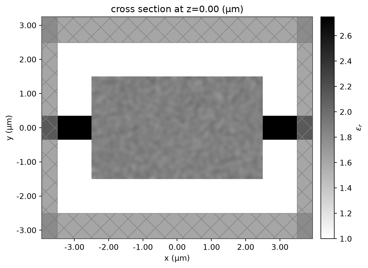
Select Input and Output Modes
Next, let’s visualize the first 4 mode profiles so we can select which mode indices we want to inject and transmit.
from tidy3d.plugins.mode.web import run as run_mode_solver

num_modes = 4
mode_spec = td.ModeSpec(num_modes=num_modes)

mode_solver = ModeSolver(
    simulation=sim_start,
    plane=source_plane,
    mode_spec=td.ModeSpec(num_modes=num_modes),
    freqs=[freq0],
)
modes = run_mode_solver(mode_solver, reduce_simulation=True)
02:24:48 UTC Mode solver created with task_id='fdve-5bd80912-3dbd-491e-9870-8af29f02a42c', solver_id='mo-bca9295e-30a3-4465-a505-b4114fc25a37'.
02:24:53 UTC Mode solver status: success
Let’s visualize the modes next.
fig, axs = plt.subplots(num_modes, 3, figsize=(12, 12), tight_layout=True)
for mode_index in range(num_modes):
    vmax = 1.1 * max(
        abs(modes.field_components[n].sel(mode_index=mode_index)).max() for n in ("Ex", "Ey", "Ez")
    )
    for field_name, ax in zip(("Ex", "Ey", "Ez"), axs[mode_index]):
        field = modes.field_components[field_name].sel(mode_index=mode_index)
        field.real.plot(label="Real", ax=ax)
        field.imag.plot(ls="--", label="Imag", ax=ax)
        ax.set_title(f"index={mode_index}, {field_name}")
        ax.set_ylim(-vmax, vmax)

axs[0, 0].legend()

print("Effective index of computed modes: ", np.array(modes.n_eff))
Effective index of computed modes: [[1.57207961 1.53546344 1.30320219 1.18494033]]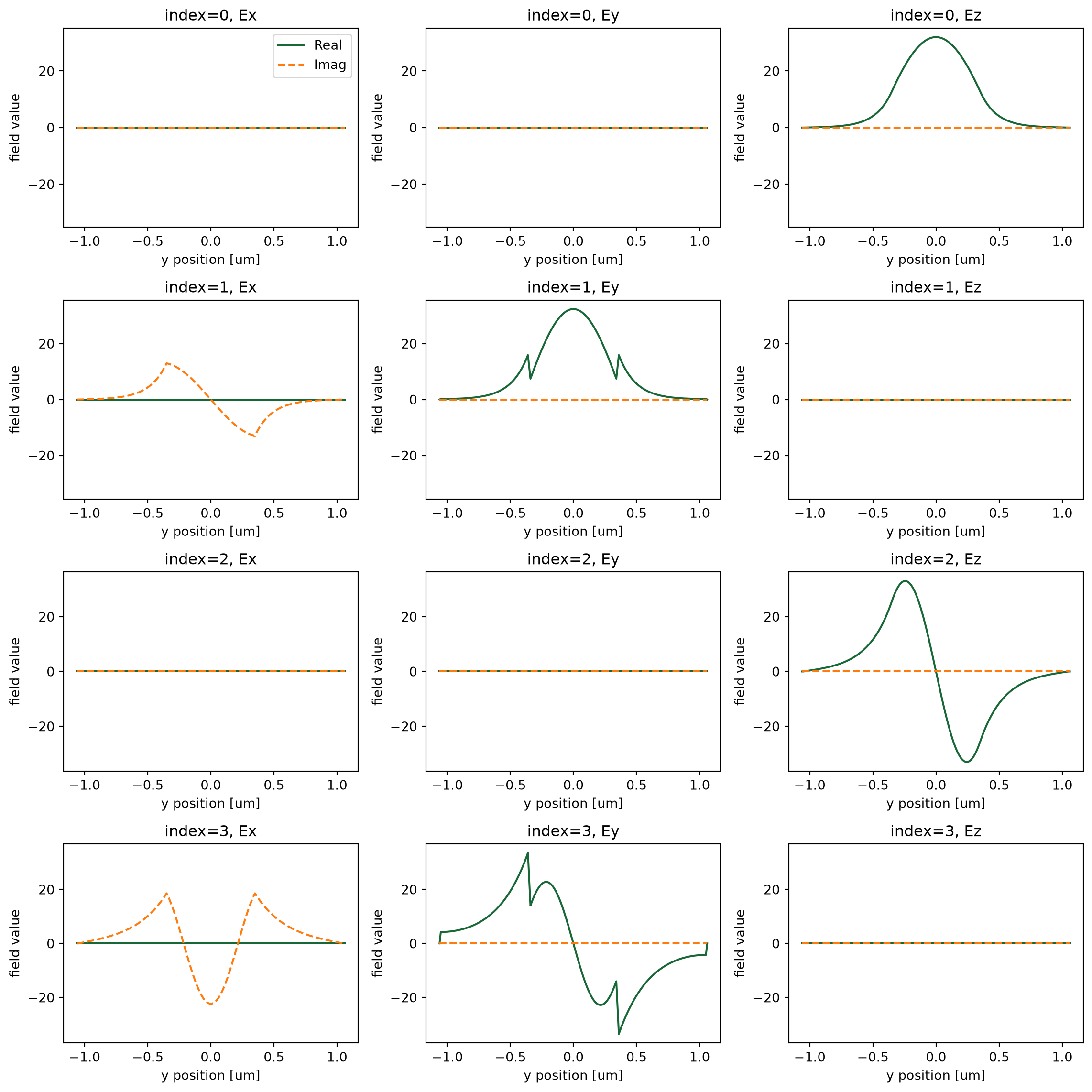
We want to inject the fundamental, Ez-polarized input into the 1st order Ez-polarized input.
From the plots, we see that these modes correspond to the first and third rows, or mode_index=0 and mode_index=2, respectively.
So we make sure that the mode_index_in and mode_index_out variables are set appropriately and we set a ModeSpec with 3 modes to be able to capture the mode_index_out in our output data.
mode_index_in = 0
mode_index_out = 2

num_modes = max(mode_index_in, mode_index_out) + 1

mode_spec = td.ModeSpec(num_modes=num_modes)
Then it is straightforward to generate our source and monitor.
# source seeding the simulation
forward_source = td.ModeSource(
    source_time=td.GaussianPulse(freq0=freq0, fwidth=freqw),
    center=[source_x, 0, 0],
    size=mode_size,
    mode_index=mode_index_in,
    mode_spec=mode_spec,
    direction="+",
)

# we'll refer to the measurement monitor by this name often
measurement_monitor_name = "measurement"

# monitor where we compute the objective function from
measurement_monitor = td.ModeMonitor(
    center=[meas_x, 0, 0],
    size=mode_size,
    freqs=[freq0],
    mode_spec=mode_spec,
    name=measurement_monitor_name,
)
Finally, we create a new function that calls our make_sim_base() function and adds the source and monitor to the result. This is the function we will use in our objective function to generate our td.Simulation given the input parameters.
def make_sim(params, beta):
    sim = make_sim_base(params, beta=beta)
    return sim.updated_copy(sources=[forward_source], monitors=[measurement_monitor])
sim_start = make_sim_base(params0, beta=1.0)
ax = sim_start.plot_eps(z=0, freq=freq0)
plt.show()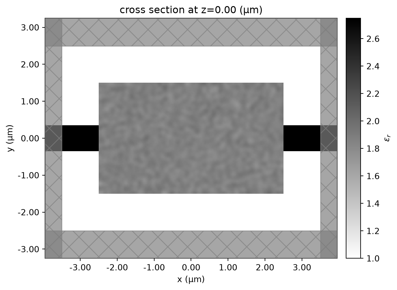
Post Processing
Next, we will define a function to tell us how we want to postprocess the output td.SimulationData object to give the conversion power that we are interested in maximizing.
def measure_power(sim_data: td.SimulationData) -> float:
    """Return the power in the output_data amplitude at the mode index of interest."""
    output_amps = sim_data["measurement"].amps
    amp = output_amps.sel(direction="+", f=freq0, mode_index=mode_index_out).values
    return anp.sum(anp.abs(amp) ** 2)
Then, we add a penalty to produce structures that are invariant under erosion and dilation, which is a useful approach to implementing minimum length scale features.
from tidy3d.plugins.autograd import make_erosion_dilation_penalty

penalty = make_erosion_dilation_penalty(radius, lx / nx)
Define Objective Function
Finally, we need to define the objective function that we want to maximize as a function of our input parameters (permittivity of each pixel) that returns the conversion power. This is the function we will differentiate later.
def J(params: np.ndarray, beta: float, step_num: int = None, verbose: bool = False) -> float:
    sim = make_sim(params, beta=beta)
    task_name = "inv_des"
    if step_num:
        task_name += f"_step_{step_num}"
    sim_data = web.run(sim, task_name=task_name, verbose=verbose)
    penalty_weight = np.minimum(1, beta / 25)
    density = filter_project(params, beta)
    return measure_power(sim_data) - penalty_weight * penalty(density)
Inverse Design
Now we are ready to perform the optimization.
We use the autograd.value_and_grad function to get the gradient of J with respect to the permittivity of each Box, while also returning the converted power associated with the current iteration, so we can record this value for later.
Let’s try running this function once to make sure it works.
dJ_fn = value_and_grad(J)val, grad = dJ_fn(params0, beta=1, verbose=True)
print(grad.shape)02:24:56 UTC Created task 'inv_des' with resource_id 'fdve-a9bb133b-c5a2-4013-8f33-c137c817e3f9' and task_type 'FDTD'.
             View task using web UI at
             'https://tidy3d.simulation.cloud/workbench?taskId=fdve-a9bb133b-c5a
             2-4013-8f33-c137c817e3f9'.
Task folder: 'default'.
02:25:00 UTC status = success
02:25:01 UTC Loading results from simulation_data.hdf5
02:25:02 UTC Started working on Batch containing 1 tasks.
02:25:06 UTC Maximum FlexCredit cost: 0.025 for the whole batch.
             Use 'Batch.real_cost()' to get the billed FlexCredit cost after
             completion.
02:25:07 UTC Batch complete.
(500, 300)print(grad)[[ 1.30448261e-08 2.56903664e-08 2.49141140e-08 ... -5.51629851e-09
-5.60823861e-09 -2.82917994e-09]
[ 2.62371350e-08 5.17052012e-08 5.01801370e-08 ... -1.10785725e-08
-1.12887450e-08 -5.69075189e-09]
[ 2.68753026e-08 5.30190434e-08 5.13777893e-08 ... -1.13478585e-08
-1.16443314e-08 -5.88133180e-09]
...
[ 3.53361651e-07 7.07449686e-07 7.15411750e-07 ... -6.03453366e-07
-5.92602692e-07 -2.94517981e-07]
[ 3.51756452e-07 7.04237935e-07 7.12308030e-07 ... -5.96807541e-07
-5.85891073e-07 -2.91144280e-07]
[ 1.75669459e-07 3.51709179e-07 3.55678365e-07 ... -2.97327931e-07
-2.91850742e-07 -1.45027304e-07]]Optimization
We will use “Adam” optimization strategy to perform sequential updates of each of the permittivity values in the td.CustomMedium.
For more information on what we use to implement this method, see this article.
We will run 10 steps and measure both the permittivities and powers at each iteration.
We run this process explicitly below with Tidy3D’s built-in Adam optimizer.
from tidy3d.plugins.autograd import adam, apply_updates

# hyperparameters
num_steps = 20
learning_rate = 1.0

# initialize adam optimizer with starting parameters
params = np.array(params0)
optimizer = adam(learning_rate=learning_rate)
opt_state = optimizer.init(params)

# store history
Js = []
params_history = [params]
beta_history = []

# gradually increase the binarization strength
beta0 = 1
beta_increment = 1

for i in range(num_steps):
    # compute gradient and current objective function value

    density = filter_project(params, beta)
    plt.subplots(figsize=(2, 2))
    plt.imshow(np.flipud(1 - density.T), cmap="gray")
    plt.axis("off")
    plt.show()

    beta = beta0 + i * beta_increment
    value, gradient = dJ_fn(params, step_num=i + 1, beta=beta)

    # outputs
    print(f"step = {i + 1}")
    print(f"\tbeta = {beta:.4e}")
    print(f"\tJ = {value:.4e}")
    print(f"\tgrad_norm = {np.linalg.norm(gradient):.4e}")

    # compute and apply updates to the optimizer based on gradient (-1 sign to maximize obj_fn)
    updates, opt_state = optimizer.update(-gradient, opt_state, params)
    params[:] = apply_updates(params, updates)

    # cap the parameters
    anp.clip(params, 0.0, 1.0, out=params)

    # save history
    Js.append(value)
    params_history.append(params.copy())
    beta_history.append(beta)

power = J(params_history[-1], beta=beta)
Js.append(power)
step = 1
    beta = 1.0000e+00
    J = -3.9947e-02
    grad_norm = 4.5917e-04
step = 2
    beta = 2.0000e+00
    J = 3.1480e-02
    grad_norm = 1.0610e-02
step = 3
    beta = 3.0000e+00
    J = -5.4355e-02
    grad_norm = 6.1677e-03
step = 4
    beta = 4.0000e+00
    J = 5.6307e-02
    grad_norm = 9.3058e-03
step = 5
    beta = 5.0000e+00
    J = 6.9386e-02
    grad_norm = 1.6097e-02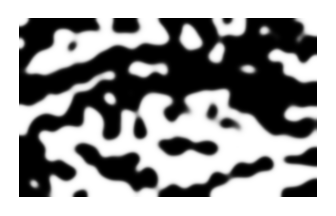
step = 6
    beta = 6.0000e+00
    J = 2.2943e-01
    grad_norm = 1.6629e-02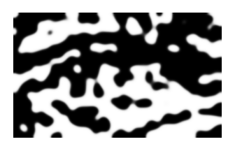
step = 7
    beta = 7.0000e+00
    J = 4.9024e-01
    grad_norm = 1.6406e-02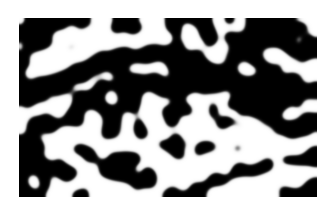
step = 8
    beta = 8.0000e+00
    J = 5.9994e-01
    grad_norm = 2.1607e-02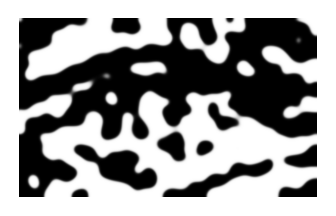
step = 9
    beta = 9.0000e+00
    J = 5.7640e-01
    grad_norm = 2.4422e-02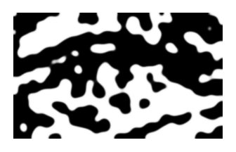
step = 10
    beta = 1.0000e+01
    J = 7.5068e-01
    grad_norm = 1.4602e-02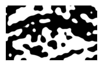
step = 11
    beta = 1.1000e+01
    J = 7.8085e-01
    grad_norm = 1.7791e-02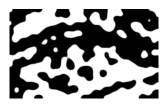
step = 12
    beta = 1.2000e+01
    J = 8.4139e-01
    grad_norm = 9.4568e-03
step = 13
    beta = 1.3000e+01
    J = 8.6675e-01
    grad_norm = 6.9955e-03
step = 14
    beta = 1.4000e+01
    J = 8.8689e-01
    grad_norm = 4.6217e-03
step = 15
    beta = 1.5000e+01
    J = 8.9377e-01
    grad_norm = 4.3625e-03
step = 16
    beta = 1.6000e+01
    J = 9.0225e-01
    grad_norm = 3.3305e-03
step = 17
    beta = 1.7000e+01
    J = 9.0796e-01
    grad_norm = 3.3380e-03
step = 18
    beta = 1.8000e+01
    J = 9.1349e-01
    grad_norm = 3.1476e-03
step = 19
    beta = 1.9000e+01
    J = 9.1941e-01
    grad_norm = 2.8195e-03
step = 20
    beta = 2.0000e+01
    J = 9.2072e-01
    grad_norm = 4.4324e-03
params_final = params_history[-1]Let’s run the optimize function.
and then record the final power value (including the last iteration’s parameter updates).
Results
First, we plot the objective function (power converted to 1st order mode) as a function of step and notice that it converges nicely!
plt.plot(Js)
plt.xlabel("iterations")
plt.ylabel("objective function")
plt.show()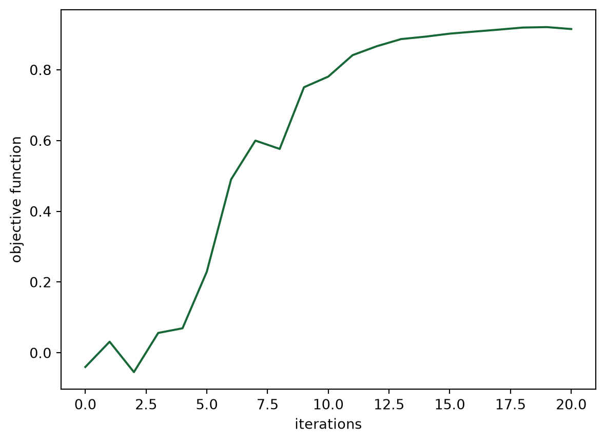
We then will visualize the final structure, so we convert it to a regular Simulation using the final permittivity values and plot it.
sim_final = make_sim(params_final, beta=beta)sim_final.plot_eps(z=0, freq=freq0)
plt.show()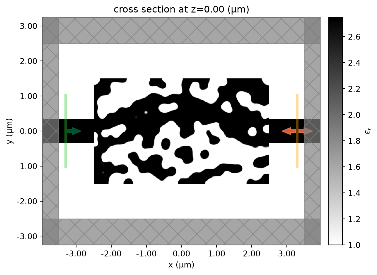
Finally, we want to inspect the fields, so we add a field monitor to the Simulation and perform one more run to record the field values for plotting.
field_mnt = td.FieldMonitor(
    size=(td.inf, td.inf, 0),
    freqs=[freq0],
    name="field_mnt",
)

sim_final = sim_final.copy(update=dict(monitors=(field_mnt, measurement_monitor)))
sim_data_final = web.run(sim_final, task_name="inv_des_final")02:29:25 UTC Created task 'inv_des_final' with resource_id 'fdve-70c55991-2e8e-48ae-b4f7-50a55e6cb387' and task_type 'FDTD'.
             View task using web UI at
             'https://tidy3d.simulation.cloud/workbench?taskId=fdve-70c55991-2e8
             e-48ae-b4f7-50a55e6cb387'.
Task folder: 'default'.
02:29:27 UTC Estimated FlexCredit cost: 0.025. This assumes the FDTD solver runs
             for the full simulation time; if early shutoff is reached, the
             billed cost can be lower. Use 'web.real_cost(task_id)' to get the
             billed FlexCredit cost after a simulation run.
02:29:28 UTC status = success
02:29:30 UTC Loading results from simulation_data.hdf5
We notice that the behavior is as expected and the device performs exactly how we intended!
f, (ax0, ax1, ax2) = plt.subplots(1, 3, figsize=(12, 3), tight_layout=True)
sim_final.plot_eps(z=0.01, freq=freq0, ax=ax0)
ax1 = sim_data_final.plot_field("field_mnt", "Ez", z=0, ax=ax1)
ax2 = sim_data_final.plot_field("field_mnt", "E", "abs^2", z=0, ax=ax2)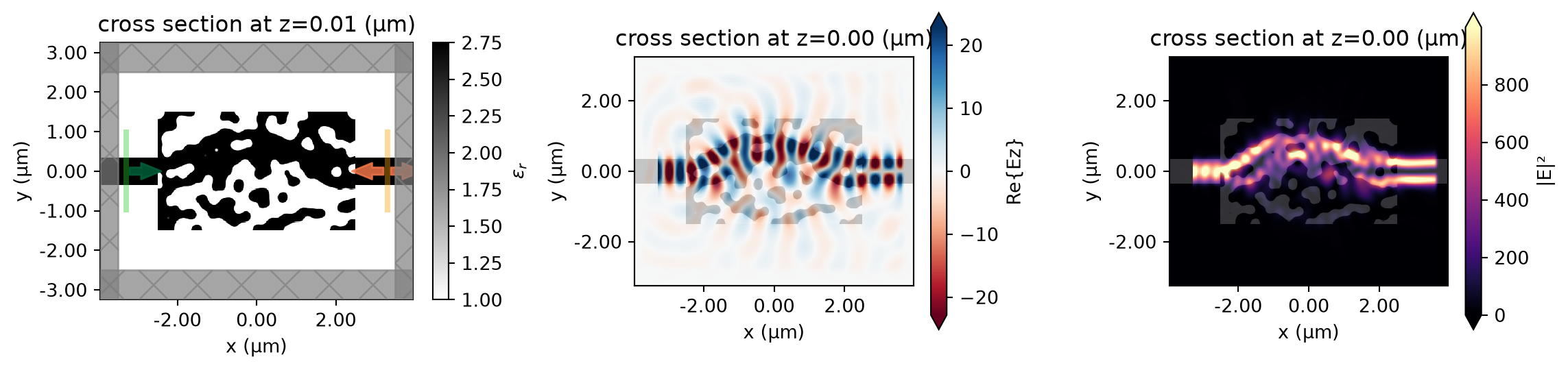
The final device converts more than 90% of the input power to the 1st mode, up from < 1% when we started.
final_power = (
    sim_data_final["measurement"].amps.sel(direction="+", f=freq0, mode_index=mode_index_out).abs
    ** 2
)
print(f"Final power conversion = {final_power * 100:.2f}%")
Final power conversion = 95.98%Export to GDS
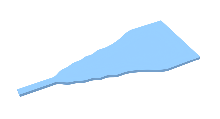
The Simulation object has the .to_gds_file convenience function to export the final design to a GDS file. In addition to a file name, it is necessary to set a cross-sectional plane (z = 0 in this case) on which to evaluate the geometry, a frequency to evaluate the permittivity, and a permittivity_threshold to define the shape boundaries in custom mediums. See the GDS export notebook for a detailed example on using .to_gds_file and other GDS related functions.
sim_final.to_gds_file(
    fname="./misc/inv_des_mode_conv.gds",
    z=0,
    frequency=freq0,
    permittivity_threshold=2.6,
)


 TERMS & CONDITIONS


 How the process works:
 Try this real URL to see an example: