





# Standard python imports.
import pickle
from typing import List

# Import autograd to be able to use automatic differentiation.
import autograd.numpy as anp
import gdstk
import matplotlib.pylab as plt
import numpy as np

# Import regular tidy3d.
import tidy3d as td
import tidy3d.web as web
from autograd import grad
from autograd.tracer import getval
from tidy3d.plugins.autograd import adam, apply_updates, optimize, value_and_grad

plt.rcParams["font.size"] = "12"
TIDY3D
LEARNING CENTER
Example Library

Parameterized level set optimization of a y-branch
Note: the cost of running the entire notebook is higher than 1 FlexCredit.
This notebook demonstrates how to set up and run a parameterized level set-based optimization of a Y-branch. In this approach, we use autograd to generate a level set surface \(\phi(\rho)\) given a set of control knots \(\rho\). The permittivity distribution is then obtained implicitly from the zero level set isocontour. Details about the level set method can be found here. Minimum gap and curvature penalty terms are introduced in the optimization to control the minimum feature size, hence improving device fabrication. In addition, we show how to tailor the initial level set function to a starting geometry, which is helpful to further optimize a device obtained by conventional design.
You can also find some interesting adjoint functionalities for shape optimization in Inverse design optimization of a waveguide taper and Adjoint-based shape optimization of a waveguide bend. If you are new to the finite-difference time-domain (FDTD) method, we highly recommend going through our FDTD101 tutorials. FDTD simulations can diverge due to various reasons. If you run into any simulation divergence issues, please follow the steps outlined in our troubleshooting guide to resolve it.

Let’s start by importing the Python libraries used throughout this notebook.
Y-branch Inverse Design Configuration
The y-branch splits the power from an input waveguide into two other output waveguides. Here, we are considering a gap of 0.3 \(\mu m\) between the output waveguides for illustration purposes. However, when considering the design of a practical device, this value can be smaller. S-bends are included to keep the output waveguides apart from each other to prevent mode coupling.
Next, you can set the y-branch geometry and the inverse design parameters.
# Geometric parameters.
y_width = 1.7  # Y-branch maximum width (um).
y_length = 1.7  # Y-branch maximum length (um).
w_thick = 0.22  # Waveguide thickness (um).
w_width = 0.5  # Waveguide width (um).
w_length = 1.0  # Input output waveguide length (um).
w_gap = 0.3  # Gap between the output waveguides (um).
bend_length = 3  # Output waveguide bend length (um).
bend_offset = 0.5  # Offset between output bends (um).

# Material.
nSi = 3.48  # Silicon refractive index.

# Inverse design set up parameters.
grid_size = 0.016  # Simulation grid size on design region (um).
ls_grid_size = 0.004  # Discretization size of the level set function (um).
ls_down_sample = (
    20  # The spacing between the level set control knots is given by ls_grid_size*ls_down_sample.
)
fom_name_1 = "fom_field1"  # Name of the monitor used to compute the objective function.
min_feature_size = 0.14  # Minimum fabrication feature size (um).
gap_par = 1.0  # Parameter to minimum gap fabrication constraint.
curve_par = 1.5  # Parameter of minimum curvature fabrication constraint.

# Optimizer parameters.
iterations = 100  # Maximum number of iterations in optimization.
learning_rate = 0.03

# Simulation wavelength.
wl = 1.55  # Central simulation wavelength (um).
bw = 0.06  # Simulation bandwidth (um).
n_wl = 61  # Number of wavelength points within the bandwidth.
From the parameters defined before, a lot of variables are computed and used to set up the optimization.
# Minimum and maximum values for the permittivities.
eps_max = nSi**2
eps_min = 1.0

# Material definition.
mat_si = td.Medium(permittivity=eps_max)  # Waveguide material.

# Wavelengths and frequencies.
wl_max = wl + bw / 2
wl_min = wl - bw / 2
wl_range = np.linspace(wl_min, wl_max, n_wl)
freq = td.C_0 / wl
freqs = td.C_0 / wl_range
freqw = 0.5 * (freqs[0] - freqs[-1])
run_time = 8e-13

# Computational domain size.
pml_spacing = 0.6 * wl
size_x = 2 * w_length + y_length + bend_length
size_y = w_gap + 2 * (bend_offset + w_width + pml_spacing)
size_z = w_thick + 2 * pml_spacing
eff_inf = 10

# Source and monitor positions.
mon_w = 3 * w_width
mon_h = 5 * w_thick

# Separation between the level set control knots.
rho_size = ls_down_sample * ls_grid_size

# Number of points on the parameter grid (rho) and level set grid (phi)
nx_rho = int(y_length / rho_size) + 1
ny_rho = int(y_width / rho_size / 2) + 1
nx_phi = int(y_length / ls_grid_size) + 1
ny_phi = int(y_width / ls_grid_size / 2) + 1
npar = nx_rho * ny_rho
ny_rho *= 2
ny_phi *= 2

# Design region size
dr_size_x = (nx_phi - 1) * ls_grid_size
dr_size_y = (ny_phi - 1) * ls_grid_size
dr_center_x = -size_x / 2 + w_length + dr_size_x / 2

# xy coordinates of the parameter and level set grids.
x_rho = np.linspace(dr_center_x - dr_size_x / 2, dr_center_x + dr_size_x / 2, nx_rho)
x_phi = np.linspace(dr_center_x - dr_size_x / 2, dr_center_x + dr_size_x / 2, nx_phi)
y_rho = np.linspace(-dr_size_y / 2, dr_size_y / 2, ny_rho)
y_phi = np.linspace(-dr_size_y / 2, dr_size_y / 2, ny_phi)
Level Set Functions
We are using autograd to implement a parameterized level set function so the gradients can be back-propagated from the permittivity distribution defined by the zero level set isocontour to the design variables (the control knots of the level set surface). The space between the control knots and the Gaussian function width obtains some control over the minimum feature size. Other types of radial basis functions can also be used in replacement of the Gaussian one employed here, such as multiquadric splines or b-splines.
class LevelSetInterp:
    """This class implements the level set surface using Gaussian radial basis functions."""

    def __init__(
        self,
        x0: anp.ndarray = None,
        y0: anp.ndarray = None,
        z0: anp.ndarray = None,
        sigma: float = None,
    ):
        # Input data.
        x, y = anp.meshgrid(y0, x0)
        xy0 = anp.column_stack((x.reshape(-1), y.reshape(-1)))
        self.xy0 = xy0
        self.z0 = z0
        self.sig = sigma
        # Builds the level set interpolation model.
        gauss_kernel = self.gaussian(self.xy0, self.xy0)
        self.model = anp.dot(anp.linalg.inv(gauss_kernel), self.z0)

    def gaussian(self, xyi, xyj):
        dist = anp.sqrt(
            (xyi[:, 1].reshape(-1, 1) - xyj[:, 1].reshape(1, -1)) ** 2
            + (xyi[:, 0].reshape(-1, 1) - xyj[:, 0].reshape(1, -1)) ** 2
        )
        return anp.exp(-(dist**2) / (2 * self.sig**2))

    def get_ls(self, x1, y1):
        xx, yy = anp.meshgrid(y1, x1)
        xy1 = anp.column_stack((xx.reshape(-1), yy.reshape(-1)))
        ls = self.gaussian(self.xy0, xy1).T @ self.model
        return ls


# Function to plot the level set surface.
def plot_level_set(x0, y0, rho, x1, y1, phi):
    y, x = np.meshgrid(y0, x0)
    yy, xx = np.meshgrid(y1, x1)

    fig = plt.figure(figsize=(12, 6), tight_layout=True)
    ax1 = fig.add_subplot(1, 2, 1, projection="3d")
    ax1.view_init(elev=45, azim=-45, roll=0)
    ax1.plot_surface(xx, yy, phi, cmap="RdBu", alpha=0.8)
    ax1.contourf(
        xx,
        yy,
        phi,
        levels=[np.amin(phi), 0],
        zdir="z",
        offset=0,
        colors=["k", "w"],
        alpha=0.5,
    )
    ax1.contour3D(xx, yy, phi, 1, cmap="binary", linewidths=[2])
    ax1.scatter(x, y, rho, color="black", linewidth=1.0)
    ax1.set_title("Level set surface")
    ax1.set_xlabel(r"x ($\mu m$)")
    ax1.set_ylabel(r"y ($\mu m$)")
    ax1.xaxis.pane.fill = False
    ax1.yaxis.pane.fill = False
    ax1.zaxis.pane.fill = False
    ax1.xaxis.pane.set_edgecolor("w")
    ax1.yaxis.pane.set_edgecolor("w")
    ax1.zaxis.pane.set_edgecolor("w")

    ax2 = fig.add_subplot(1, 2, 2)
    ax2.contourf(xx, yy, phi, levels=[0, np.amax(phi)], colors=[[0, 0, 0]])
    ax2.set_title("Zero level set contour")
    ax2.set_xlabel(r"x ($\mu m$)")
    ax2.set_ylabel(r"y ($\mu m$)")
    ax2.set_aspect("equal")
    plt.show()
To map the permittivities to the zero-level set contour and obtain continuous derivatives, we use a hyperbolic tangent function as an approximation to a Heaviside function. Other smooth functions, such as sigmoid and arctangent, can also be employed. As discussed here, the difference on computed interface using different functions will decrease when reducing the mesh size.
def mirror_param(design_param):
    param = anp.array(design_param).reshape((nx_rho, int(ny_rho / 2)))

    try:
        param_minus = param._value.copy()
    except:
        param_minus = param.copy()

    return anp.concatenate((anp.fliplr(param_minus), param), axis=1).flatten()


def get_eps(design_param, sharpness=10.0, plot_levelset=False) -> np.ndarray:
    """Returns the permittivities defined by the zero level set isocontour"""
    phi_model = LevelSetInterp(x0=x_rho, y0=y_rho, z0=design_param, sigma=rho_size)
    phi = phi_model.get_ls(x1=x_phi, y1=y_phi)

    # Calculates the permittivities from the level set surface
    eps_phi = 0.5 * (anp.tanh(sharpness * phi) + 1)
    eps = eps_min + (eps_max - eps_min) * eps_phi
    eps = anp.maximum(eps, eps_min)
    eps = anp.minimum(eps, eps_max)

    # Reshapes the design parameters into a 2D matrix.
    eps = anp.reshape(eps, (nx_phi, ny_phi))

    # Plots the level set surface.
    if plot_levelset:
        rho = np.reshape(design_param, (nx_rho, ny_rho))
        phi = np.reshape(phi, (nx_phi, ny_phi))
        plot_level_set(x0=x_rho, y0=y_rho, rho=rho, x1=x_phi, y1=y_phi, phi=phi)

    return eps
In the next function, the permittivity values are used to build a CustomMedium within the design region.
def update_design(eps, unfold=False) -> List[td.Structure]:
    # Reflects the structure about the x-axis.
    eps_val = anp.array(eps).reshape((nx_phi, ny_phi, 1))
    coords_x = [(dr_center_x - dr_size_x / 2) + ix * ls_grid_size for ix in range(nx_phi)]

    if not unfold:
        # Creation of a CustomMedium using the values of the design parameters.
        coords_yp = [0 + iy * ls_grid_size for iy in range(int(ny_phi / 2))]
        coords = dict(x=coords_x, y=coords_yp, z=[0])
        eps_ag = td.SpatialDataArray(eps_val, coords=coords)
        eps_medium = td.CustomMedium(permittivity=eps_ag)
        box = td.Box(
            center=(dr_center_x, dr_size_y / 4, 0),
            size=(dr_size_x, dr_size_y / 2, w_thick),
        )
        structure = [td.Structure(geometry=box, medium=eps_medium)]

    else:
        # Creation of a CustomMedium using the values of the design parameters.
        coords_y = [-dr_size_y / 2 + iy * ls_grid_size for iy in range(ny_phi)]
        coords = dict(x=coords_x, y=coords_y, z=[0])
        eps_ag = td.SpatialDataArray(eps_val, coords=coords)
        eps_medium = td.CustomMedium(permittivity=eps_ag)
        box = td.Box(center=(dr_center_x, 0, 0), size=(dr_size_x, dr_size_y, w_thick))
        structure = [td.Structure(geometry=box, medium=eps_medium)]
    return structure
Initial Structure
We built an initial y-brach structure containing some holes and different gap sizes to demonstrate how the design evolves under fabrication constraints. We define this structure using a PolySlab object and then translate it into a permittivity grid of the same size as the one used to define the level set function. The holes are introduced in the polygon using the ClipOperation object.
vertices = np.array(
    [
        (-size_x / 2 + w_length, w_width / 2),
        (-size_x / 2 + w_length + 0.5, w_width / 2),
        (-size_x / 2 + w_length + 0.75, w_gap / 2 + w_width),
        (-size_x / 2 + w_length + dr_size_x, w_gap / 2 + w_width),
        (-size_x / 2 + w_length + dr_size_x, w_gap / 2),
        (-size_x / 2 + w_length + 2.5 * dr_size_x / 3, w_gap / 2),
        (-size_x / 2 + w_length + 2.3 * dr_size_x / 3, w_gap / 6),
        (-size_x / 2 + w_length + 1.8 * dr_size_x / 3, w_gap / 6),
        (-size_x / 2 + w_length + 1.8 * dr_size_x / 3, -w_gap / 6),
        (-size_x / 2 + w_length + 2.3 * dr_size_x / 3, -w_gap / 6),
        (-size_x / 2 + w_length + 2.5 * dr_size_x / 3, -w_gap / 2),
        (-size_x / 2 + w_length + dr_size_x, -w_gap / 2),
        (-size_x / 2 + w_length + dr_size_x, -w_gap / 2 - w_width),
        (-size_x / 2 + w_length + 0.75, -w_gap / 2 - w_width),
        (-size_x / 2 + w_length + 0.5, -w_width / 2),
        (-size_x / 2 + w_length, -w_width / 2),
    ]
)

y_poly = td.PolySlab(vertices=vertices, axis=2, slab_bounds=(-w_thick / 2, w_thick / 2))
y_hole1 = td.Cylinder(
    center=(
        -size_x / 2 + w_length + 1.7 * dr_size_x / 3,
        w_gap / 2 + w_width / 1.75,
        0,
    ),
    radius=min_feature_size / 3,
    length=w_thick,
    axis=2,
)
y_hole2 = td.Cylinder(
    center=(
        -size_x / 2 + w_length + 1.7 * dr_size_x / 3,
        -w_gap / 2 - w_width / 1.75,
        0,
    ),
    radius=min_feature_size / 3,
    length=w_thick,
    axis=2,
)
y_hole3 = td.Cylinder(
    center=(
        -size_x / 2 + w_length + 2.3 * dr_size_x / 3,
        w_gap / 2 + w_width / 1.75,
        0,
    ),
    radius=min_feature_size / 1.5,
    length=w_thick,
    axis=2,
)
y_hole4 = td.Cylinder(
    center=(
        -size_x / 2 + w_length + 2.3 * dr_size_x / 3,
        -w_gap / 2 - w_width / 1.75,
        0,
    ),
    radius=min_feature_size / 1.5,
    length=w_thick,
    axis=2,
)
init_design = td.ClipOperation(operation="difference", geometry_a=y_poly, geometry_b=y_hole1)
init_design = td.ClipOperation(operation="difference", geometry_a=init_design, geometry_b=y_hole2)
init_design = td.ClipOperation(operation="difference", geometry_a=init_design, geometry_b=y_hole3)
init_design = td.ClipOperation(operation="difference", geometry_a=init_design, geometry_b=y_hole4)

init_eps = init_design.inside_meshgrid(x=x_phi, y=y_phi, z=np.zeros(1))
init_eps = np.squeeze(init_eps) * eps_max

init_design.plot(z=0)
plt.show()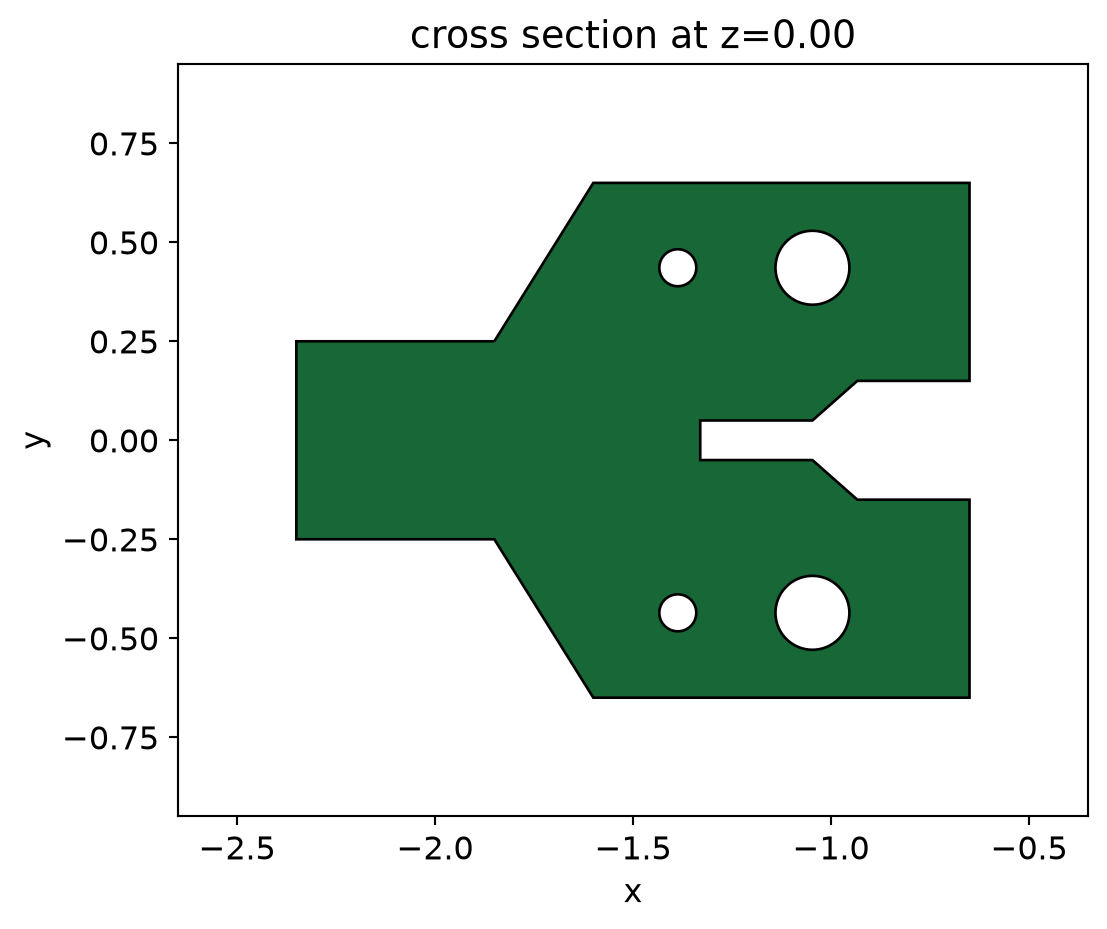
Then an objective function which compares the initial structure and the permittivity distribution generated by the level set zero contour is defined.
# Figure of Merit (FOM) calculation.
def fom_eps(eps_ref: anp.ndarray, eps: anp.ndarray) -> float:
    """Calculate the L2 norm between eps_ref and eps."""
    return anp.mean(anp.abs(eps_ref - eps) ** 2)


# Objective function to be passed to the optimization algorithm.
def obj_eps(design_param, eps_ref) -> float:
    param = mirror_param(design_param)
    eps = get_eps(param)
    return fom_eps(eps_ref, eps)


# Function to calculate the objective function value and its
# gradient with respect to the design parameters.
obj_grad_eps = value_and_grad(obj_eps)
So, the initial control knots are obtained after fitting the initial structure using the level set function. This is accomplished by minimizing the L2 norm between the reference and the level set generated permittivities with Tidy3D’s built-in Adam optimizer.
# Initialize adam optimizer with starting parameters.
start_par = np.zeros(npar)


def fit_objective(design_param):
    return obj_eps(design_param, init_eps)


def report_step(params_eps, gradient, state, step_index, objective_val):
    print(f"Step = {step_index + 1}")
    print(f"\tobj_eps = {objective_val:.4e}")
    print(f"\tgrad_norm = {np.linalg.norm(gradient):.4e}")


params_eps, opt_state, history = optimize(
    fit_objective,
    params0=np.copy(start_par),
    optimizer=adam(learning_rate=learning_rate * 10),
    num_steps=50,
    callback=report_step,
)

# Gets the final parameters and the objective values history.
init_rho = np.copy(params_eps)
obj_eps = list(history["objective_fn_val"])
obj_vals_eps = np.array(obj_eps)
Step = 1
obj_eps = 3.6660e+01
grad_norm = 2.1337e+01
Step = 2
obj_eps = 3.8352e+00
grad_norm = 1.6936e+00
Step = 3
obj_eps = 2.5730e+00
grad_norm = 9.9866e-01
Step = 4
obj_eps = 2.2393e+00
grad_norm = 8.5924e-01
Step = 5
obj_eps = 2.0405e+00
grad_norm = 7.2283e-01
Step = 6
obj_eps = 1.7910e+00
grad_norm = 5.7900e-01
Step = 7
obj_eps = 1.5631e+00
grad_norm = 4.3837e-01
Step = 8
obj_eps = 1.4112e+00
grad_norm = 3.6683e-01
Step = 9
obj_eps = 1.3339e+00
grad_norm = 3.5290e-01
Step = 10
obj_eps = 1.3045e+00
grad_norm = 3.7025e-01
Step = 11
obj_eps = 1.2842e+00
grad_norm = 3.8085e-01
Step = 12
obj_eps = 1.2494e+00
grad_norm = 3.7093e-01
Step = 13
obj_eps = 1.1982e+00
grad_norm = 3.4043e-01
Step = 14
obj_eps = 1.1420e+00
grad_norm = 3.0237e-01
Step = 15
obj_eps = 1.0898e+00
grad_norm = 2.6239e-01
Step = 16
obj_eps = 1.0486e+00
grad_norm = 2.2298e-01
Step = 17
obj_eps = 1.0252e+00
grad_norm = 2.0291e-01
Step = 18
obj_eps = 1.0168e+00
grad_norm = 2.0348e-01
Step = 19
obj_eps = 1.0145e+00
grad_norm = 2.1126e-01
Step = 20
obj_eps = 1.0113e+00
grad_norm = 2.1521e-01
Step = 21
obj_eps = 1.0042e+00
grad_norm = 2.1250e-01
Step = 22
obj_eps = 9.9248e-01
grad_norm = 2.0371e-01
Step = 23
obj_eps = 9.7660e-01
grad_norm = 1.8586e-01
Step = 24
obj_eps = 9.5979e-01
grad_norm = 1.6358e-01
Step = 25
obj_eps = 9.4568e-01
grad_norm = 1.5022e-01
Step = 26
obj_eps = 9.3461e-01
grad_norm = 1.4719e-01
Step = 27
obj_eps = 9.2473e-01
grad_norm = 1.4254e-01
Step = 28
obj_eps = 9.1579e-01
grad_norm = 1.3176e-01
Step = 29
obj_eps = 9.0934e-01
grad_norm = 1.2223e-01
Step = 30
obj_eps = 9.0622e-01
grad_norm = 1.1917e-01
Step = 31
obj_eps = 9.0575e-01
grad_norm = 1.2233e-01
Step = 32
obj_eps = 9.0587e-01
grad_norm = 1.2684e-01
Step = 33
obj_eps = 9.0428e-01
grad_norm = 1.2751e-01
Step = 34
obj_eps = 8.9978e-01
grad_norm = 1.2027e-01
Step = 35
obj_eps = 8.9303e-01
grad_norm = 1.0461e-01
Step = 36
obj_eps = 8.8631e-01
grad_norm = 8.4469e-02
Step = 37
obj_eps = 8.8203e-01
grad_norm = 7.0780e-02
Step = 38
obj_eps = 8.8096e-01
grad_norm = 7.4915e-02
Step = 39
obj_eps = 8.8144e-01
grad_norm = 8.7472e-02
Step = 40
obj_eps = 8.8084e-01
grad_norm = 9.4230e-02
Step = 41
obj_eps = 8.7774e-01
grad_norm = 9.0045e-02
Step = 42
obj_eps = 8.7278e-01
grad_norm = 7.6119e-02
Step = 43
obj_eps = 8.6799e-01
grad_norm = 5.9258e-02
Step = 44
obj_eps = 8.6511e-01
grad_norm = 5.1587e-02
Step = 45
obj_eps = 8.6431e-01
grad_norm = 5.6978e-02
Step = 46
obj_eps = 8.6438e-01
grad_norm = 6.4243e-02
Step = 47
obj_eps = 8.6399e-01
grad_norm = 6.5571e-02
Step = 48
obj_eps = 8.6270e-01
grad_norm = 6.0462e-02
Step = 49
obj_eps = 8.6095e-01
grad_norm = 5.2884e-02
Step = 50
obj_eps = 8.5943e-01
grad_norm = 4.8189e-02The following graph shows the evolution of the objective function along the initial structure fitting.
fig, ax = plt.subplots(1, 1, figsize=(6, 4))
ax.plot(obj_vals_eps, "ro")
ax.set_xlabel("iterations")
ax.set_ylabel("objective function")
ax.set_title(f"Level Set Fit: Obj = {obj_vals_eps[-1]:.3f}")
ax.set_yscale("log")
plt.show()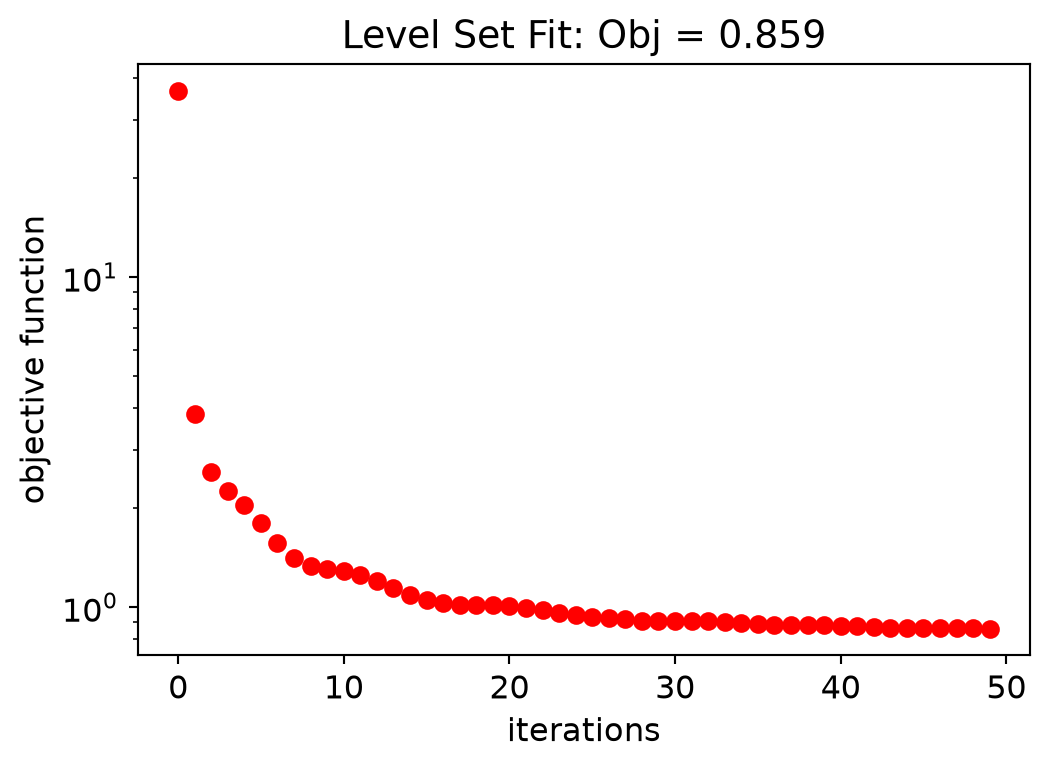
Here, one can see the initial parameters, which are the control knots defining the level set surface. The geometry of the structure will change as the zero isocontour evolves. The width of the Gaussian radial basis functions and the spacing of the control knots impact the accuracy and the smoothness of the initial zero-level set contour.
eps_fit = get_eps(mirror_param(init_rho), plot_levelset=True)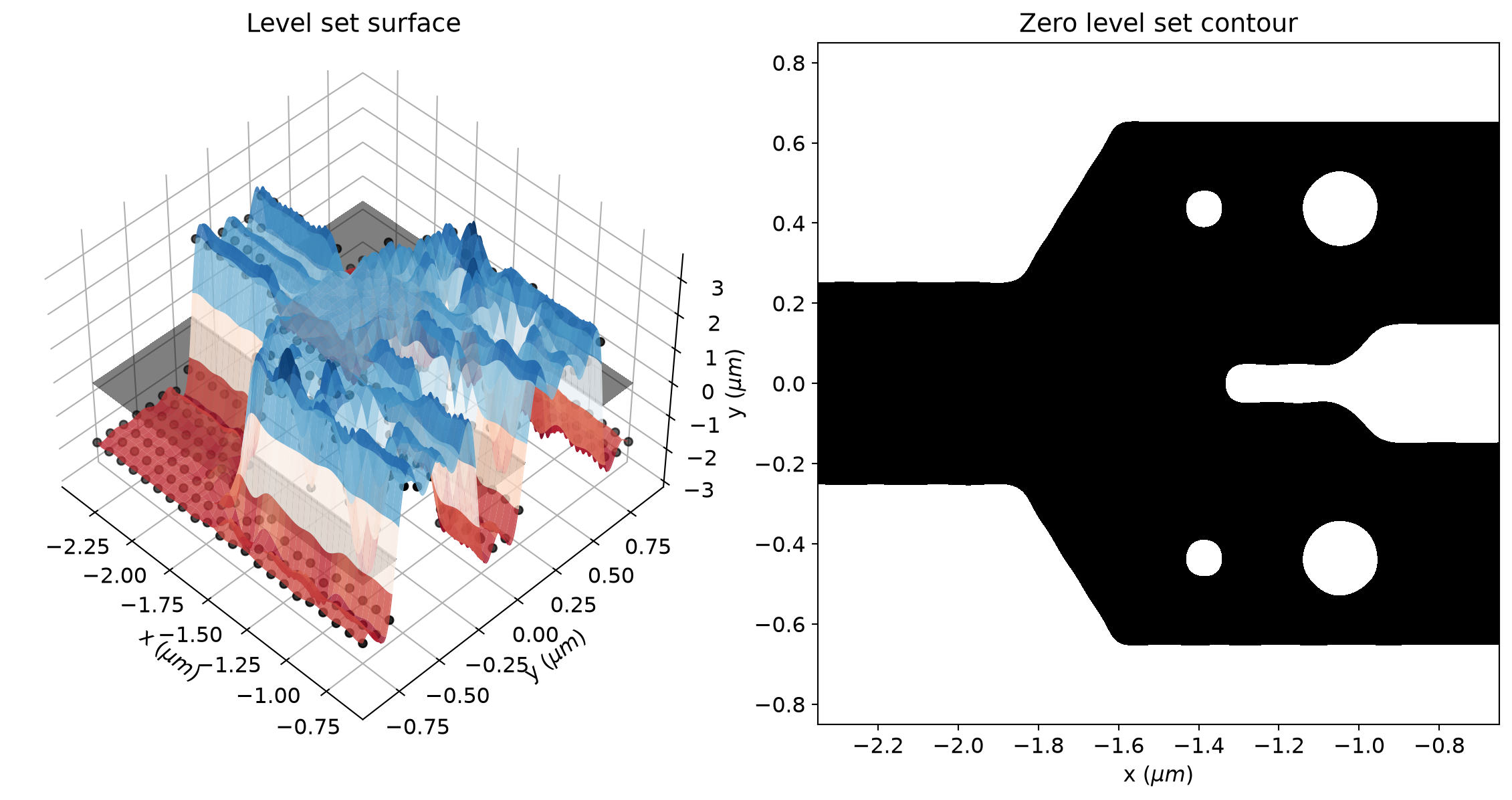
Inverse Design Optimization Set Up
Next, we will write a function to return the Simulation object. Note that we are using a MeshOverrideStructure to obtain a uniform mesh over the design region.
The elements that do not change along the optimization are defined first.
# Input waveguide.
wg_input = td.Structure(
    geometry=td.Box.from_bounds(
        rmin=(-eff_inf, -w_width / 2, -w_thick / 2),
        rmax=(-size_x / 2 + w_length + grid_size, w_width / 2, w_thick / 2),
    ),
    medium=mat_si,
)

# Output bends.
x_start = (
    -size_x / 2 + w_length + dr_size_x - grid_size
)  # x-coordinate of the starting point of the waveguide bends.
x = np.linspace(x_start, x_start + bend_length, 100)  # x-coordinates of the top edge vertices.
y = (
    (x - x_start) * bend_offset / bend_length
    - bend_offset * np.sin(2 * np.pi * (x - x_start) / bend_length) / (np.pi * 2)
    + (w_gap + w_width) / 2
)  # y coordinates of the top edge vertices

# adding the last point to include the straight waveguide at the output
x = np.append(x, eff_inf)
y = np.append(y, y[-1])

# add path to the cell
cell = gdstk.Cell("bend")
cell.add(gdstk.FlexPath(x + 1j * y, w_width, layer=1, datatype=0))  # Top waveguide bend.
cell.add(gdstk.FlexPath(x - 1j * y, w_width, layer=1, datatype=0))  # Bottom waveguide bend.

# Define top waveguide bend structure.
wg_bend_top = td.Structure(
    geometry=td.PolySlab.from_gds(
        cell,
        gds_layer=1,
        axis=2,
        slab_bounds=(-w_thick / 2, w_thick / 2),
    )[1],
    medium=mat_si,
)

# Define bottom waveguide bend structure.
wg_bend_bot = td.Structure(
    geometry=td.PolySlab.from_gds(
        cell,
        gds_layer=1,
        axis=2,
        slab_bounds=(-w_thick / 2, w_thick / 2),
    )[0],
    medium=mat_si,
)
Monitors used to get simulation data.
# Input mode source.
mode_spec = td.ModeSpec(num_modes=1, target_neff=nSi)
source = td.ModeSource(
    center=(-size_x / 2 + 0.15 * wl, 0, 0),
    size=(0, mon_w, mon_h),
    source_time=td.GaussianPulse(freq0=freq, fwidth=freqw),
    direction="+",
    mode_spec=mode_spec,
    mode_index=0,
)

# Monitor where we will compute the objective function from.
fom_monitor_1 = td.ModeMonitor(
    center=[size_x / 2 - 0.25 * wl, (w_gap + w_width) / 2 + bend_offset, 0],
    size=[0, mon_w, mon_h],
    freqs=[freq],
    mode_spec=mode_spec,
    name=fom_name_1,
)

# Monitors used only to visualize the initial and final y-branch results.
# Field monitors to visualize the final fields.
field_xy = td.FieldMonitor(
    size=(td.inf, td.inf, 0),
    freqs=[freq],
    name="field_xy",
)

# Monitor where we will compute the objective function from.
fom_final_1 = td.ModeMonitor(
    center=[size_x / 2 - 0.25 * wl, (w_gap + w_width) / 2 + bend_offset, 0],
    size=[0, mon_w, mon_h],
    freqs=freqs,
    mode_spec=mode_spec,
    name="out_1",
)
And then the Simulation is built.
def make_adjoint_sim(design_param, unfold=True) -> td.Simulation:
    # Builds the design region from the design parameters.
    eps = get_eps(design_param)
    design_structure = update_design(eps, unfold=unfold)

    # Creates a uniform mesh for the design region.
    adjoint_dr_mesh = td.MeshOverrideStructure(
        geometry=td.Box(center=(dr_center_x, 0, 0), size=(dr_size_x, dr_size_y, w_thick)),
        dl=[grid_size, grid_size, grid_size],
        enforce=True,
    )

    return td.Simulation(
        size=[size_x, size_y, size_z],
        center=[0, 0, 0],
        grid_spec=td.GridSpec.auto(
            wavelength=wl_max,
            min_steps_per_wvl=15,
            override_structures=[adjoint_dr_mesh],
        ),
        symmetry=(0, -1, 1),
        structures=[wg_input, wg_bend_top, wg_bend_bot] + design_structure,
        sources=[source],
        monitors=[fom_monitor_1],
        run_time=run_time,
        subpixel=True,
    )
Let’s visualize the simulation setup and verify if all the elements are in their correct places. Differently from the density-based methods, we will start from a fully binarized structure.
init_design = make_adjoint_sim(mirror_param(init_rho), unfold=True)

fig, ax1 = plt.subplots(1, 1, tight_layout=True, figsize=(8, 5))
init_design.plot_eps(z=0, ax=ax1)
plt.show()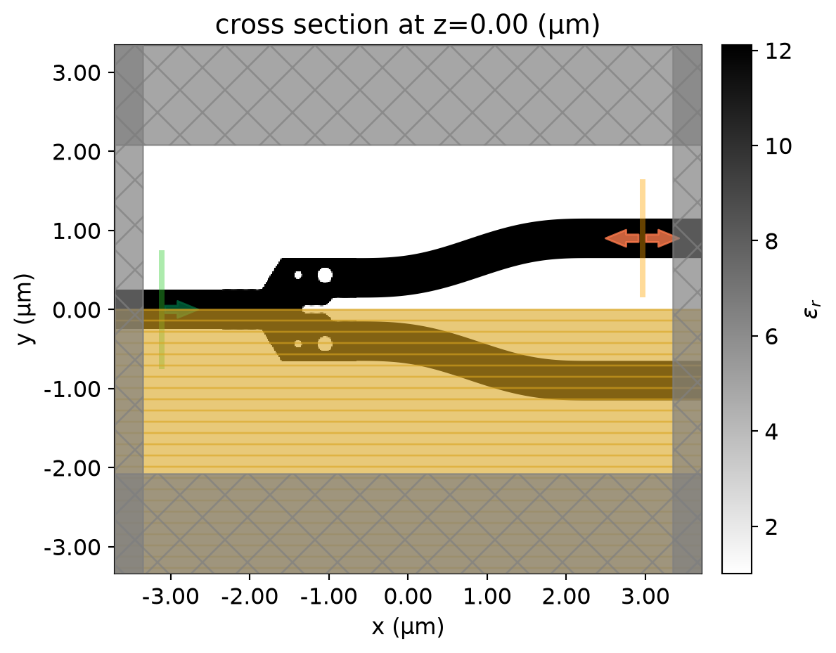
Now, we will run a simulation to see how this non-optimized y-branch performs.
sim_init = init_design.copy(update=dict(monitors=(field_xy, fom_final_1)))
sim_data = web.run(sim_init, task_name="initial y-branch")
20:47:29 UTC Created task 'initial y-branch' with resource_id 'fdve-89b9344a-f090-47a2-b1ad-4e578d7d1e7f' and task_type 'FDTD'.
             View task using web UI at
             'https://tidy3d.simulation.cloud/workbench?taskId=fdve-89b9344a-f09
             0-47a2-b1ad-4e578d7d1e7f'.
Task folder: 'default'.
20:47:31 UTC Estimated FlexCredit cost: 0.025. This assumes the FDTD solver runs
             for the full simulation time; if early shutoff is reached, the
             billed cost can be lower. Use 'web.real_cost(task_id)' to get the
             billed FlexCredit cost after a simulation run.
20:47:32 UTC status = success
20:47:33 UTC Loading results from simulation_data.hdf5
We will use the insertion loss (IL) to compare the device response before and after the optimization. Since we will use symmetry about the y-axis, the insertion loss is calculated as \(IL = -10 log(2P_{1}/P_{in})\), where \(P_{1}\) is the power coupled into the upper s-bend and \(P_{in}\) is the unit input power. The insertion loss of the non-optimized y-branch is above 3 dB at 1.55 \(\mu m\). From the field distribution image, we can realize that it happens because much of the input power is reflected.
coeffs_f = sim_data["out_1"].amps.sel(direction="+")
power_1 = np.abs(coeffs_f.sel(mode_index=0)) ** 2
power_1_db = -10 * np.log10(2 * power_1)

f, (ax1, ax2) = plt.subplots(1, 2, figsize=(9, 4), tight_layout=True)
ax1.plot(wl_range, power_1_db, "-k")
ax1.set_xlabel("Wavelength (um)")
ax1.set_ylabel("Power (dB)")
ax1.set_ylim(0, 4)
ax1.set_xlim(wl - bw / 2, wl + bw / 2)
ax1.set_title("Insertion Loss")
sim_data.plot_field("field_xy", "E", "abs^2", z=0, ax=ax2)
plt.show()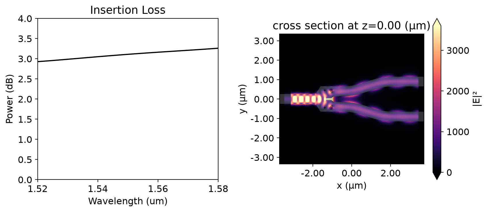
Fabrication Constraints
Fabrication constraints are introduced in the optimization as penalty terms to control the minimum gap (\(f_{g}\)) and radius of curvature (\(f_{c}\)) in the final design. Below, we use autograd to define the penalty terms following the formulation presented in D. Vercruysse, N. V. Sapra, L. Su, R. Trivedi, and J. Vučković, "Analytical level set fabrication constraints for inverse design," Scientific Reports 9, 8999 (2019). DOI: 10.1038/s41598-019-45026-0. The gap penalty function controls the minimum feature size by limiting the second derivative based on the value of the function at that point. The curvature constraint is only relevant at the device boundary, where \(\phi = 0\), so we apply the smoothed Heaviside function to the level set surface before calculating the derivatives.
# Auxiliary function to calculate first and second order partial derivatives.
def ls_derivatives(phi, d_size):
    SC = 1e-12
    phi_1 = anp.array(anp.gradient(phi)) / d_size
    phi_x = phi_1[0] + SC
    phi_y = phi_1[1] + SC
    phi_2x = anp.array(anp.gradient(phi_x)) / d_size
    phi_2y = anp.array(anp.gradient(phi_y)) / d_size

    phi_xx = phi_2x[0]
    phi_xy = phi_2x[1]
    phi_yy = phi_2y[1]
    return phi_x, phi_y, phi_xx, phi_xy, phi_yy


# Minimum gap size fabrication constraint integrand calculation.
# The "beta" parameter relax the constraint near the zero plane.
def fab_penalty_ls_gap(params, beta=1, min_feature_size=min_feature_size, grid_size=ls_grid_size):
    # Get the level set surface.
    phi_model = LevelSetInterp(x0=x_rho, y0=y_rho, z0=params, sigma=rho_size)
    phi = phi_model.get_ls(x1=x_phi, y1=y_phi)
    phi = anp.reshape(phi, (nx_phi, ny_phi))

    # Calculates their derivatives.
    phi_x, phi_y, phi_xx, phi_xy, phi_yy = ls_derivatives(phi, grid_size)

    # Calculates the gap penalty over the level set grid.
    pi_d = np.pi / (1.3 * min_feature_size)
    phi_v = anp.maximum(anp.power(phi_x**2 + phi_y**2, 0.5), anp.power(1e-32, 1 / 4))
    phi_vv = (phi_x**2 * phi_xx + 2 * phi_x * phi_y * phi_xy + phi_y**2 * phi_yy) / phi_v**2
    return (
        anp.maximum((anp.abs(phi_vv) / (pi_d * anp.abs(phi) + beta * phi_v) - pi_d), 0)
        * grid_size**2
    )


# Minimum radius of curvature fabrication constraint integrand calculation.
# The "alpha" parameter controls its relative weight to the gap penalty.
# The "sharpness" parameter controls the smoothness of the surface near the zero-contour.
def fab_penalty_ls_curve(
    params,
    alpha=1,
    sharpness=1,
    min_feature_size=min_feature_size,
    grid_size=ls_grid_size,
):
    # Get the permittivity surface and calculates their derivatives.
    eps = get_eps(params, sharpness=sharpness)
    eps_x, eps_y, eps_xx, eps_xy, eps_yy = ls_derivatives(eps, grid_size)

    # Calculates the curvature penalty over the permittivity grid.
    pi_d = np.pi / (1.1 * min_feature_size)
    eps_v = anp.maximum(anp.sqrt(eps_x**2 + eps_y**2), anp.power(1e-32, 1 / 6))
    k = (eps_x**2 * eps_yy - 2 * eps_x * eps_y * eps_xy + eps_y**2 * eps_xx) / eps_v**3
    curve_const = anp.abs(k * anp.arctan(eps_v / eps)) - pi_d
    curve_const = anp.nan_to_num(curve_const)
    return alpha * anp.maximum(curve_const, 0) * grid_size**2


# Gap and curvature fabrication constraints calculation.
# Penalty values are normalized by "norm_gap" and "norm_curve".
def fab_penalty_ls(
    params,
    beta=gap_par,
    alpha=curve_par,
    sharpness=4,
    min_feature_size=min_feature_size,
    grid_size=ls_grid_size,
    norm_gap=1,
    norm_curve=1,
):
    # Get the gap penalty fabrication constraint value.
    gap_penalty_int = fab_penalty_ls_gap(
        params=params, beta=beta, min_feature_size=min_feature_size, grid_size=grid_size
    )
    gap_penalty_int = anp.nan_to_num(gap_penalty_int)

    gap_penalty = anp.sum(gap_penalty_int) / norm_gap

    # Get the curvature penalty fabrication constraint value.
    curve_penalty_int = fab_penalty_ls_curve(
        params=params,
        alpha=alpha,
        sharpness=sharpness,
        min_feature_size=min_feature_size,
        grid_size=grid_size,
    )

    curve_penalty_int = anp.nan_to_num(curve_penalty_int)
    curve_penalty = anp.sum(curve_penalty_int) / norm_curve

    return gap_penalty, curve_penalty
Now, we will calculate the initial penalty function values and observe the regions of the initial design that violate the constraints. The gap and curvature penalty functions are normalized by their initial values along the optimization to better balance the weights of device response and fabrication penalty within the objective function.
# Initial values of gap and curvature fabrication constraints.
init_fab_gap, init_fab_curve = fab_penalty_ls(mirror_param(init_rho))

# Visualization of gap and curvature fabrication constraints values.
gap_penalty_int = fab_penalty_ls_gap(mirror_param(init_rho), beta=gap_par)
curve_penalty_int = fab_penalty_ls_curve(mirror_param(init_rho), alpha=curve_par, sharpness=4)

fig, (ax1, ax2) = plt.subplots(1, 2, figsize=(12, 8), tight_layout=True)
yy, xx = np.meshgrid(y_phi, x_phi)

im = ax1.imshow(
    np.flipud(gap_penalty_int.T),
    extent=[x_phi[0], x_phi[-1], y_phi[0], y_phi[-1]],
    interpolation="none",
    cmap="gnuplot2_r",
)
ax1.contour(xx, yy, eps_fit, [(eps_min + eps_max) / 2], colors="k", linewidths=0.5)
ax1.set_title(f"Gap Penalty = {init_fab_gap:.3f}")
ax1.set_xlabel(r"x ($\mu m$)")
ax1.set_ylabel(r"y ($\mu m$)")
fig.colorbar(im, ax=ax1, shrink=0.3)

im = ax2.imshow(
    anp.flipud(curve_penalty_int.T),
    extent=[x_phi[0], x_phi[-1], y_phi[0], y_phi[-1]],
    interpolation="none",
    cmap="gnuplot2_r",
)
ax2.contour(xx, yy, eps_fit, [(eps_min + eps_max) / 2], colors="k", linewidths=0.5)
ax2.set_title(f"Curve Penalty = {init_fab_curve:.3f}")
ax2.set_xlabel(r"x ($\mu m$)")
ax2.set_ylabel(r"y ($\mu m$)")
fig.colorbar(im, ax=ax2, shrink=0.3)
plt.show()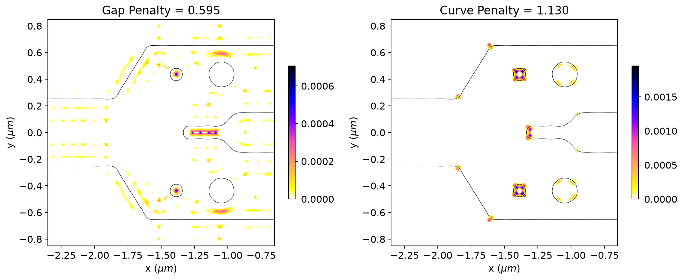
Running the Optimization
The figure-of-merit used in the y-branch optimization is the power (\(P_{1, 2}\)) coupled into the fundamental transverse electric mode of the output waveguides. We will set mirror symmetry about the y-axis in the optimization, so we must include only \(P_{1}\) in the figure-of-merit. As we are using a minimization strategy, the coupled power and fabrication constraints are arranged within the objective function as \(|0.5 - P_{1}| + w_{f} \times (f_{g} + f_{c})\), where \(w_{f}\) is the fabrication constraint weight, whereas \(f_{g}\) and \(f_{c}\) are the gap and curvature penalty values.
# Figure of Merit (FOM) calculation.
def fom(sim_data: td.SimulationData) -> float:
    """Return the power at the mode index of interest."""
    output_amps1 = sim_data[fom_name_1].amps
    amp1 = output_amps1.sel(direction="+", f=freq, mode_index=0)
    eta1 = anp.sum(anp.nan_to_num(anp.abs(amp1.values)) ** 2)
    return anp.abs(0.5 - eta1), eta1


# Objective function to be passed to the optimization algorithm.
def obj(
    design_param,
    fab_const: float = 0.0,
    norm_gap=1.0,
    norm_curve=1.0,
    verbose: bool = False,
) -> float:
    param = mirror_param(design_param)
    sim = make_adjoint_sim(param)
    sim_data = web.run(sim, task_name="inv_des_ybranch", verbose=verbose)
    fom_val, eta1 = fom(sim_data)
    fab_gap, fab_curve = fab_penalty_ls(param, norm_gap=norm_gap, norm_curve=norm_curve)
    J = fom_val + fab_const * (fab_gap + fab_curve)
    aux_data = anp.array([sim_data, getval(eta1), getval(fab_gap), getval(fab_curve)])

    return (J, aux_data)


# Function to calculate the objective function value and its
# gradient with respect to the design parameters.
obj_grad = value_and_grad(obj, has_aux=True)
Optimizer initialization
# where to store history
history_fname = "./misc/y_branch_fab.pkl"


def save_history(history_dict: dict) -> None:
    """Convenience function to save the history to file."""
    with open(history_fname, "wb") as file:
        pickle.dump(history_dict, file)


def load_history() -> dict:
    """Convenience method to load the history from file."""
    with open(history_fname, "rb") as file:
        history_dict = pickle.load(file)
    return history_dict
Before starting, we will look for data from a previous optimization.
# Initialize adam optimizer with starting parameters.
optimizer = adam(learning_rate=learning_rate * 8)

try:
    history_dict = load_history()
    opt_state = history_dict["opt_states"][-1]
    params = history_dict["params"][-1]
    num_iters_completed = len(history_dict["params"])
    print("Loaded optimization checkpoint from file.")
    print(f"Found {num_iters_completed} iterations previously completed out of {iterations} total.")
    if num_iters_completed < iterations:
        print("Will resume optimization.")
    else:
        print("Optimization completed, will return results.")

except (FileNotFoundError, IndexError):
    params = np.array(init_rho)
    opt_state = optimizer.init(params)
    history_dict = dict(
        values=[],
        eta1=[],
        penalty_gap=[],
        penalty_curve=[],
        params=[],
        gradients=[],
        opt_states=[opt_state],
        data=[],
    )
Now, we are ready to run the optimization!
td.config.logging.level = "WARNING"

iter_done = len(history_dict["values"])
fab_const = 0.05

param_eps = anp.array(get_eps(mirror_param(anp.array(params))))
param_shape = param_eps.shape
param_eps = param_eps.flatten()

if iter_done < iterations:
    for i in range(iter_done, iterations):
        params = anp.array(params)

        (value, gradient), aux = obj_grad(
            params,
            fab_const=fab_const,
            norm_gap=init_fab_gap,
            norm_curve=init_fab_curve,
        )
        sim_data_i, eta1, penalty_gap, penalty_curve = aux

        gradient = np.nan_to_num(gradient)
        gradient = np.array(gradient)
        params = np.array(params)

        # outputs
        print(f"Step = {i + 1}")
        print(f"\tobj_val = {value:.4e}")
        print(f"\tgrad_norm = {np.linalg.norm(gradient):.4e}")
        print(f"\teta1 = {eta1:.3f}")
        print(f"\tpenalty gap = {penalty_gap:.3f}")
        print(f"\tpenalty curve = {penalty_curve:.3f}")

        # Compute and apply updates to the optimizer based on gradient.
        updates, opt_state = optimizer.update(gradient, opt_state, params)
        params = apply_updates(params, updates)

        # Save history.
        history_dict["values"].append(value)
        history_dict["eta1"].append(eta1)
        history_dict["penalty_gap"].append(penalty_gap)
        history_dict["penalty_curve"].append(penalty_curve)
        history_dict["params"].append(params)
        history_dict["gradients"].append(gradient)
        history_dict["opt_states"].append(opt_state)
        # history_dict["data"].append(sim_data_i)  # Uncomment to store data, can create large files.
        save_history(history_dict)
Step = 1
obj_val = 3.5564e-01
grad_norm = 3.9942e-02
eta1 = 0.244
penalty gap = 1.000
penalty curve = 1.000
Step = 2
obj_val = 3.0409e-01
grad_norm = 3.7730e-02
eta1 = 0.280
penalty gap = 0.508
penalty curve = 1.179
Step = 3
obj_val = 2.7739e-01
grad_norm = 3.9409e-02
eta1 = 0.309
penalty gap = 0.553
penalty curve = 1.169
Step = 4
obj_val = 2.4488e-01
grad_norm = 3.1357e-02
eta1 = 0.339
penalty gap = 0.614
penalty curve = 1.067
Step = 5
obj_val = 2.1634e-01
grad_norm = 4.5609e-02
eta1 = 0.370
penalty gap = 0.576
penalty curve = 1.158
Step = 6
obj_val = 1.8553e-01
grad_norm = 3.4512e-02
eta1 = 0.400
penalty gap = 0.438
penalty curve = 1.276
Step = 7
obj_val = 1.5951e-01
grad_norm = 3.1326e-02
eta1 = 0.424
penalty gap = 0.413
penalty curve = 1.256
Step = 8
obj_val = 1.4281e-01
grad_norm = 1.8774e-02
eta1 = 0.439
penalty gap = 0.380
penalty curve = 1.250
Step = 9
obj_val = 1.3151e-01
grad_norm = 1.6255e-02
eta1 = 0.449
penalty gap = 0.361
penalty curve = 1.242
Step = 10
obj_val = 1.2360e-01
grad_norm = 1.5448e-02
eta1 = 0.456
penalty gap = 0.382
penalty curve = 1.206
Step = 11
obj_val = 1.1775e-01
grad_norm = 1.5583e-02
eta1 = 0.462
penalty gap = 0.415
penalty curve = 1.182
Step = 12
obj_val = 1.1323e-01
grad_norm = 2.0103e-02
eta1 = 0.466
penalty gap = 0.429
penalty curve = 1.156
Step = 13
obj_val = 1.0730e-01
grad_norm = 1.5568e-02
eta1 = 0.470
penalty gap = 0.426
penalty curve = 1.119
Step = 14
obj_val = 1.0346e-01
grad_norm = 1.6143e-02
eta1 = 0.473
penalty gap = 0.435
penalty curve = 1.101
Step = 15
obj_val = 1.0034e-01
grad_norm = 1.3805e-02
eta1 = 0.475
penalty gap = 0.432
penalty curve = 1.083
Step = 16
obj_val = 9.6688e-02
grad_norm = 1.2034e-02
eta1 = 0.478
penalty gap = 0.433
penalty curve = 1.069
Step = 17
obj_val = 9.4373e-02
grad_norm = 1.0315e-02
eta1 = 0.480
penalty gap = 0.438
penalty curve = 1.058
Step = 18
obj_val = 9.2759e-02
grad_norm = 8.8639e-03
eta1 = 0.482
penalty gap = 0.446
penalty curve = 1.050
Step = 19
obj_val = 8.9755e-02
grad_norm = 9.0138e-03
eta1 = 0.483
penalty gap = 0.425
penalty curve = 1.039
Step = 20
obj_val = 8.7463e-02
grad_norm = 1.2173e-02
eta1 = 0.484
penalty gap = 0.396
penalty curve = 1.037
Step = 21
obj_val = 8.4831e-02
grad_norm = 1.3942e-02
eta1 = 0.486
penalty gap = 0.372
penalty curve = 1.037
Step = 22
obj_val = 8.1774e-02
grad_norm = 1.0431e-02
eta1 = 0.488
penalty gap = 0.353
penalty curve = 1.037
Step = 23
obj_val = 8.0195e-02
grad_norm = 8.1543e-03
eta1 = 0.489
penalty gap = 0.345
penalty curve = 1.038
Step = 24
obj_val = 7.8613e-02
grad_norm = 7.7371e-03
eta1 = 0.490
penalty gap = 0.336
penalty curve = 1.029
Step = 25
obj_val = 7.7383e-02
grad_norm = 7.5870e-03
eta1 = 0.490
penalty gap = 0.326
penalty curve = 1.014
Step = 26
obj_val = 7.5177e-02
grad_norm = 7.5547e-03
eta1 = 0.490
penalty gap = 0.313
penalty curve = 0.988
Step = 27
obj_val = 7.2747e-02
grad_norm = 6.4796e-03
eta1 = 0.490
penalty gap = 0.291
penalty curve = 0.964
Step = 28
obj_val = 7.0961e-02
grad_norm = 6.7225e-03
eta1 = 0.490
penalty gap = 0.273
penalty curve = 0.938
Step = 29
obj_val = 6.9815e-02
grad_norm = 7.8602e-03
eta1 = 0.489
penalty gap = 0.260
penalty curve = 0.919
Step = 30
obj_val = 6.8537e-02
grad_norm = 7.9626e-03
eta1 = 0.489
penalty gap = 0.250
penalty curve = 0.900
Step = 31
obj_val = 6.7119e-02
grad_norm = 5.2158e-03
eta1 = 0.489
penalty gap = 0.241
penalty curve = 0.881
Step = 32
obj_val = 6.5843e-02
grad_norm = 4.6583e-03
eta1 = 0.489
penalty gap = 0.229
penalty curve = 0.861
Step = 33
obj_val = 6.4888e-02
grad_norm = 4.7265e-03
eta1 = 0.488
penalty gap = 0.222
penalty curve = 0.843
Step = 34
obj_val = 6.4107e-02
grad_norm = 4.4880e-03
eta1 = 0.488
penalty gap = 0.222
penalty curve = 0.823
Step = 35
obj_val = 6.3048e-02
grad_norm = 5.4165e-03
eta1 = 0.488
penalty gap = 0.218
penalty curve = 0.806
Step = 36
obj_val = 6.1777e-02
grad_norm = 4.3972e-03
eta1 = 0.488
penalty gap = 0.210
penalty curve = 0.790
Step = 37
obj_val = 6.0325e-02
grad_norm = 4.5535e-03
eta1 = 0.488
penalty gap = 0.198
penalty curve = 0.775
Step = 38
obj_val = 5.9262e-02
grad_norm = 5.8577e-03
eta1 = 0.489
penalty gap = 0.192
penalty curve = 0.764
Step = 39
obj_val = 5.7904e-02
grad_norm = 6.2391e-03
eta1 = 0.489
penalty gap = 0.186
penalty curve = 0.750
Step = 40
obj_val = 5.7063e-02
grad_norm = 8.2078e-03
eta1 = 0.489
penalty gap = 0.181
penalty curve = 0.734
Step = 41
obj_val = 5.5912e-02
grad_norm = 9.7532e-03
eta1 = 0.489
penalty gap = 0.174
penalty curve = 0.718
Step = 42
obj_val = 5.4665e-02
grad_norm = 5.3343e-03
eta1 = 0.489
penalty gap = 0.171
penalty curve = 0.705
Step = 43
obj_val = 5.4217e-02
grad_norm = 6.7392e-03
eta1 = 0.489
penalty gap = 0.172
penalty curve = 0.696
Step = 44
obj_val = 5.3923e-02
grad_norm = 9.1929e-03
eta1 = 0.489
penalty gap = 0.170
penalty curve = 0.692
Step = 45
obj_val = 5.2491e-02
grad_norm = 5.6896e-03
eta1 = 0.490
penalty gap = 0.166
penalty curve = 0.685
Step = 46
obj_val = 5.1952e-02
grad_norm = 4.7937e-03
eta1 = 0.490
penalty gap = 0.166
penalty curve = 0.674
Step = 47
obj_val = 5.1210e-02
grad_norm = 4.4554e-03
eta1 = 0.490
penalty gap = 0.161
penalty curve = 0.662
Step = 48
obj_val = 5.0404e-02
grad_norm = 4.4619e-03
eta1 = 0.490
penalty gap = 0.156
penalty curve = 0.648
Step = 49
obj_val = 4.9155e-02
grad_norm = 5.9705e-03
eta1 = 0.490
penalty gap = 0.147
penalty curve = 0.632
Step = 50
obj_val = 4.7932e-02
grad_norm = 3.6646e-03
eta1 = 0.490
penalty gap = 0.139
penalty curve = 0.613
Step = 51
obj_val = 4.6974e-02
grad_norm = 3.2963e-03
eta1 = 0.489
penalty gap = 0.135
penalty curve = 0.594
Step = 52
obj_val = 4.6108e-02
grad_norm = 3.7570e-03
eta1 = 0.489
penalty gap = 0.129
penalty curve = 0.579
Step = 53
obj_val = 4.5469e-02
grad_norm = 5.2975e-03
eta1 = 0.489
penalty gap = 0.129
penalty curve = 0.565
Step = 54
obj_val = 4.4516e-02
grad_norm = 4.5027e-03
eta1 = 0.489
penalty gap = 0.127
penalty curve = 0.549
Step = 55
obj_val = 4.3903e-02
grad_norm = 4.3555e-03
eta1 = 0.489
penalty gap = 0.129
penalty curve = 0.535
Step = 56
obj_val = 4.3379e-02
grad_norm = 4.3322e-03
eta1 = 0.489
penalty gap = 0.129
penalty curve = 0.523
Step = 57
obj_val = 4.2920e-02
grad_norm = 4.7846e-03
eta1 = 0.489
penalty gap = 0.129
penalty curve = 0.510
Step = 58
obj_val = 4.2757e-02
grad_norm = 4.0842e-03
eta1 = 0.489
penalty gap = 0.131
penalty curve = 0.503
Step = 59
obj_val = 4.2431e-02
grad_norm = 4.1011e-03
eta1 = 0.489
penalty gap = 0.131
penalty curve = 0.497
Step = 60
obj_val = 4.1844e-02
grad_norm = 4.7127e-03
eta1 = 0.489
penalty gap = 0.130
penalty curve = 0.488
Step = 61
obj_val = 4.1167e-02
grad_norm = 4.6104e-03
eta1 = 0.489
penalty gap = 0.124
penalty curve = 0.481
Step = 62
obj_val = 4.0906e-02
grad_norm = 7.8654e-03
eta1 = 0.489
penalty gap = 0.122
penalty curve = 0.478
Step = 63
obj_val = 4.0423e-02
grad_norm = 3.8875e-03
eta1 = 0.489
penalty gap = 0.122
penalty curve = 0.469
Step = 64
obj_val = 3.9945e-02
grad_norm = 5.0190e-03
eta1 = 0.489
penalty gap = 0.119
penalty curve = 0.462
Step = 65
obj_val = 3.9724e-02
grad_norm = 4.2461e-03
eta1 = 0.489
penalty gap = 0.120
penalty curve = 0.457
Step = 66
obj_val = 3.9108e-02
grad_norm = 4.4017e-03
eta1 = 0.489
penalty gap = 0.117
penalty curve = 0.447
Step = 67
obj_val = 3.8864e-02
grad_norm = 4.7894e-03
eta1 = 0.489
penalty gap = 0.117
penalty curve = 0.443
Step = 68
obj_val = 3.8210e-02
grad_norm = 4.1860e-03
eta1 = 0.489
penalty gap = 0.109
penalty curve = 0.439
Step = 69
obj_val = 3.7943e-02
grad_norm = 3.9134e-03
eta1 = 0.489
penalty gap = 0.109
penalty curve = 0.437
Step = 70
obj_val = 3.7846e-02
grad_norm = 4.1351e-03
eta1 = 0.489
penalty gap = 0.107
penalty curve = 0.439
Step = 71
obj_val = 3.7559e-02
grad_norm = 5.4550e-03
eta1 = 0.489
penalty gap = 0.104
penalty curve = 0.437
Step = 72
obj_val = 3.6457e-02
grad_norm = 3.8221e-03
eta1 = 0.490
penalty gap = 0.103
penalty curve = 0.431
Step = 73
obj_val = 3.6270e-02
grad_norm = 6.2285e-03
eta1 = 0.490
penalty gap = 0.102
penalty curve = 0.427
Step = 74
obj_val = 3.5929e-02
grad_norm = 5.7047e-03
eta1 = 0.490
penalty gap = 0.100
penalty curve = 0.420
Step = 75
obj_val = 3.5601e-02
grad_norm = 4.2427e-03
eta1 = 0.490
penalty gap = 0.103
penalty curve = 0.414
Step = 76
obj_val = 3.5540e-02
grad_norm = 1.1907e-02
eta1 = 0.490
penalty gap = 0.107
penalty curve = 0.406
Step = 77
obj_val = 3.5696e-02
grad_norm = 1.0684e-02
eta1 = 0.490
penalty gap = 0.112
penalty curve = 0.395
Step = 78
obj_val = 3.5336e-02
grad_norm = 6.5151e-03
eta1 = 0.490
penalty gap = 0.120
penalty curve = 0.388
Step = 79
obj_val = 3.6258e-02
grad_norm = 2.2788e-02
eta1 = 0.489
penalty gap = 0.129
penalty curve = 0.382
Step = 80
obj_val = 3.5885e-02
grad_norm = 1.2025e-02
eta1 = 0.489
penalty gap = 0.136
penalty curve = 0.367
Step = 81
obj_val = 3.5564e-02
grad_norm = 1.1123e-02
eta1 = 0.489
penalty gap = 0.130
penalty curve = 0.359
Step = 82
obj_val = 3.4811e-02
grad_norm = 6.8832e-03
eta1 = 0.489
penalty gap = 0.122
penalty curve = 0.363
Step = 83
obj_val = 3.5170e-02
grad_norm = 2.0224e-02
eta1 = 0.489
penalty gap = 0.114
penalty curve = 0.368
Step = 84
obj_val = 3.4858e-02
grad_norm = 1.1793e-02
eta1 = 0.489
penalty gap = 0.110
penalty curve = 0.371
Step = 85
obj_val = 3.5314e-02
grad_norm = 1.2176e-02
eta1 = 0.489
penalty gap = 0.113
penalty curve = 0.383
Step = 86
obj_val = 3.4789e-02
grad_norm = 6.1656e-03
eta1 = 0.490
penalty gap = 0.124
penalty curve = 0.380
Step = 87
obj_val = 3.5739e-02
grad_norm = 2.0928e-02
eta1 = 0.490
penalty gap = 0.131
penalty curve = 0.374
Step = 88
obj_val = 3.4498e-02
grad_norm = 6.7771e-03
eta1 = 0.490
penalty gap = 0.131
penalty curve = 0.360
Step = 89
obj_val = 3.4650e-02
grad_norm = 1.2762e-02
eta1 = 0.489
penalty gap = 0.125
penalty curve = 0.355
Step = 90
obj_val = 3.4065e-02
grad_norm = 7.3738e-03
eta1 = 0.490
penalty gap = 0.123
penalty curve = 0.353
Step = 91
obj_val = 3.4319e-02
grad_norm = 7.3344e-03
eta1 = 0.490
penalty gap = 0.118
penalty curve = 0.366
Step = 92
obj_val = 3.4668e-02
grad_norm = 9.1308e-03
eta1 = 0.490
penalty gap = 0.118
penalty curve = 0.378
Step = 93
obj_val = 3.3697e-02
grad_norm = 7.1108e-03
eta1 = 0.490
penalty gap = 0.118
penalty curve = 0.366
Step = 94
obj_val = 3.3664e-02
grad_norm = 7.5679e-03
eta1 = 0.490
penalty gap = 0.120
penalty curve = 0.358
Step = 95
obj_val = 3.3522e-02
grad_norm = 6.7773e-03
eta1 = 0.490
penalty gap = 0.121
penalty curve = 0.359
Step = 96
obj_val = 3.3237e-02
grad_norm = 6.4506e-03
eta1 = 0.491
penalty gap = 0.121
penalty curve = 0.357
Step = 97
obj_val = 3.3189e-02
grad_norm = 1.2006e-02
eta1 = 0.490
penalty gap = 0.122
penalty curve = 0.350
Step = 98
obj_val = 3.2427e-02
grad_norm = 7.6139e-03
eta1 = 0.490
penalty gap = 0.115
penalty curve = 0.343
Step = 99
obj_val = 3.2119e-02
grad_norm = 9.3080e-03
eta1 = 0.490
penalty gap = 0.104
penalty curve = 0.342
Step = 100
obj_val = 3.1937e-02
grad_norm = 6.2338e-03
eta1 = 0.491
penalty gap = 0.104
penalty curve = 0.346obj_vals = np.array(history_dict["values"])
eta1_vals = np.array(history_dict["eta1"])
pen_gap_vals = np.array(history_dict["penalty_gap"])
pen_curve_vals = np.array(history_dict["penalty_curve"])
final_par = history_dict["params"][-1]Optimization Results
Below, we can see how the device response and fabrication penalty have evolved throughout the optimization. The coupling into the output waveguide improves quickly in the beginning at the expense of higher penalty values. Then, the penalty values decrease linearly after the device response achieves a near-optimal condition. This trend results from the small weight factor we have chosen for the fabrication penalty terms.
fig, ax = plt.subplots(1, 1, figsize=(6, 4))
ax.plot(obj_vals, "ko", label="objective")
ax.plot(eta1_vals, "bo", label="p_1")
ax.plot(pen_gap_vals, "ro", label="gap")
ax.plot(pen_curve_vals, "gs", label="curvature")
ax.set_xlabel("iterations")
ax.set_ylabel("objective function")
ax.legend()
ax.set_yscale("log")
ax.set_title(f"Final Objective Function Value: {obj_vals[-1]:.3f}")
plt.show()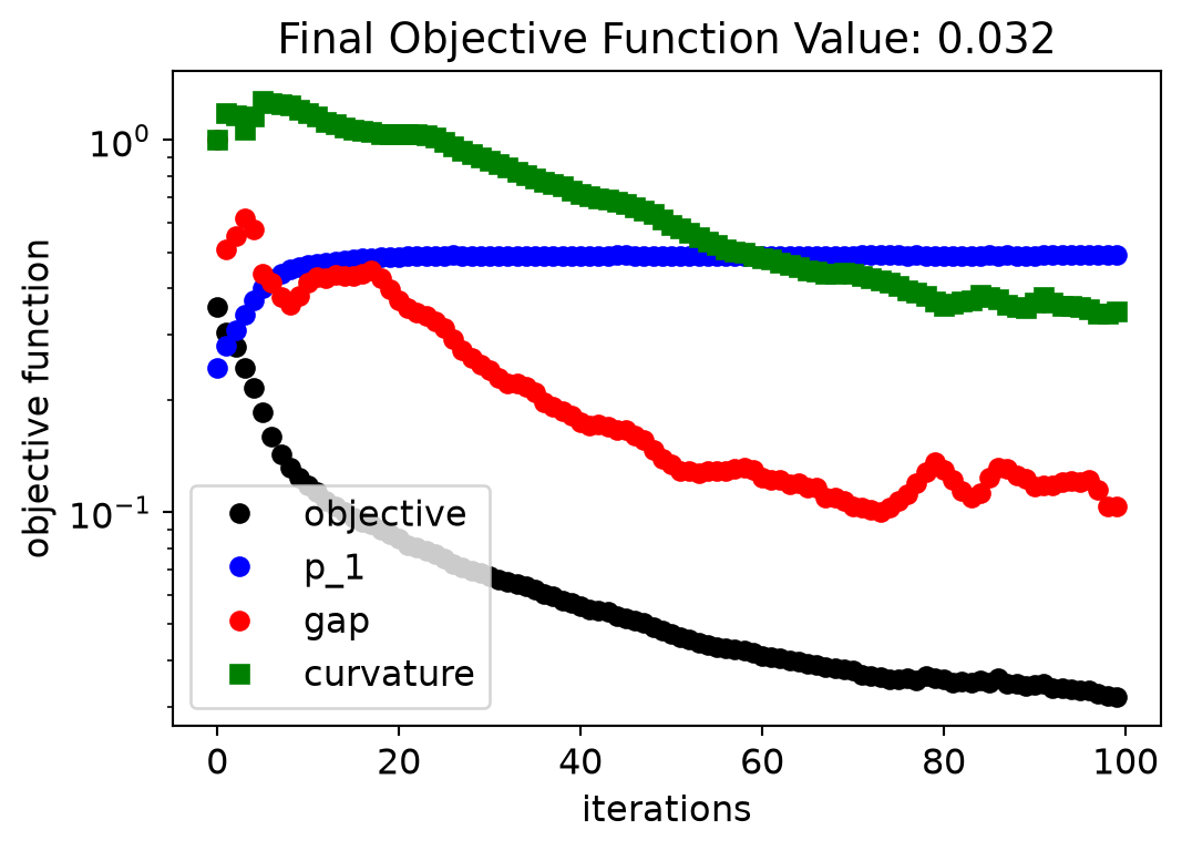
The optimization process obtained a smooth and well-defined geometry.
eps_final = get_eps(mirror_param(final_par), plot_levelset=True)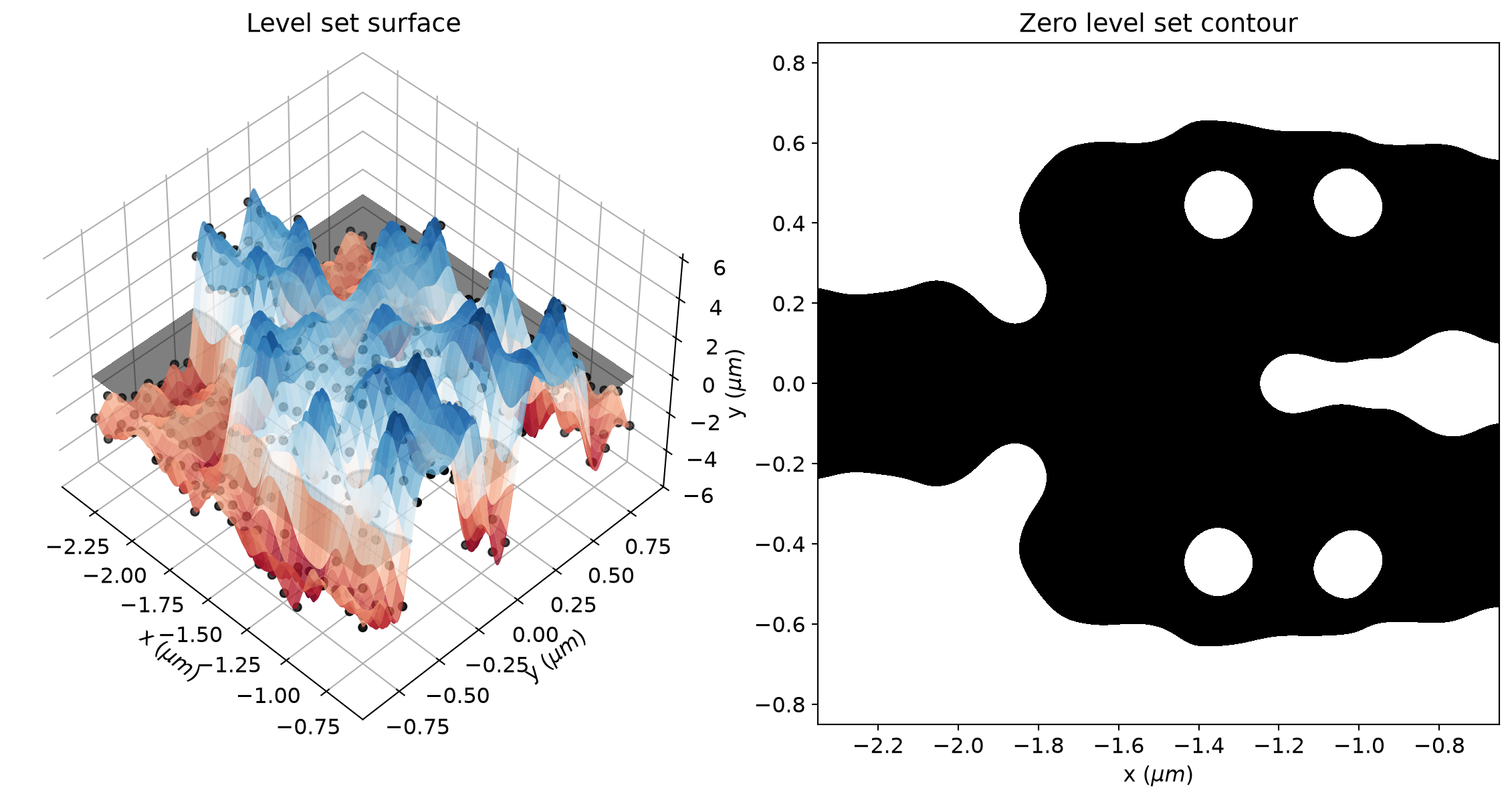
We can also see a significant reduction in violations to the minimum feature size after the optimization, which results in a smoother structure. The optimized device has not matched the minimum feature size exactly. The minimum radius of curvature and gap size are about 30% higher and 20% lower than the reference feature size, respectively. This deviation is expected, as reported in the previous paper. In this regard, running the simulation longer, adjusting the penalty weight or compensating for the reference feature size could improve the results.
# Initial values of gap and curvature fabrication constraints.
final_fab_gap, final_fab_curve = fab_penalty_ls(mirror_param(final_par))

# Visualization of gap and curvature fabrication constraints values.
gap_penalty_int = fab_penalty_ls_gap(mirror_param(final_par), beta=gap_par)
curve_penalty_int = fab_penalty_ls_curve(mirror_param(final_par), alpha=curve_par, sharpness=4)

fig, (ax1, ax2) = plt.subplots(1, 2, figsize=(12, 8), tight_layout=True)
yy, xx = np.meshgrid(y_phi, x_phi)

im = ax1.imshow(
    np.flipud(gap_penalty_int.T),
    extent=[x_phi[0], x_phi[-1], y_phi[0], y_phi[-1]],
    interpolation="none",
    cmap="gnuplot2_r",
)
ax1.contour(xx, yy, eps_final, [(eps_min + eps_max) / 2], colors="k", linewidths=0.5)
ax1.set_title(f"Gap Penalty = {final_fab_gap:.3f}")
ax1.set_xlabel(r"x ($\mu m$)")
ax1.set_ylabel(r"y ($\mu m$)")
fig.colorbar(im, ax=ax1, shrink=0.3)

im = ax2.imshow(
    anp.flipud(curve_penalty_int.T),
    extent=[x_phi[0], x_phi[-1], y_phi[0], y_phi[-1]],
    interpolation="none",
    cmap="gnuplot2_r",
)
ax2.contour(xx, yy, eps_final, [(eps_min + eps_max) / 2], colors="k", linewidths=0.5)
ax2.set_title(f"Curve Penalty = {final_fab_curve:.3f}")
ax2.set_xlabel(r"x ($\mu m$)")
ax2.set_ylabel(r"y ($\mu m$)")
fig.colorbar(im, ax=ax2, shrink=0.3)
plt.show()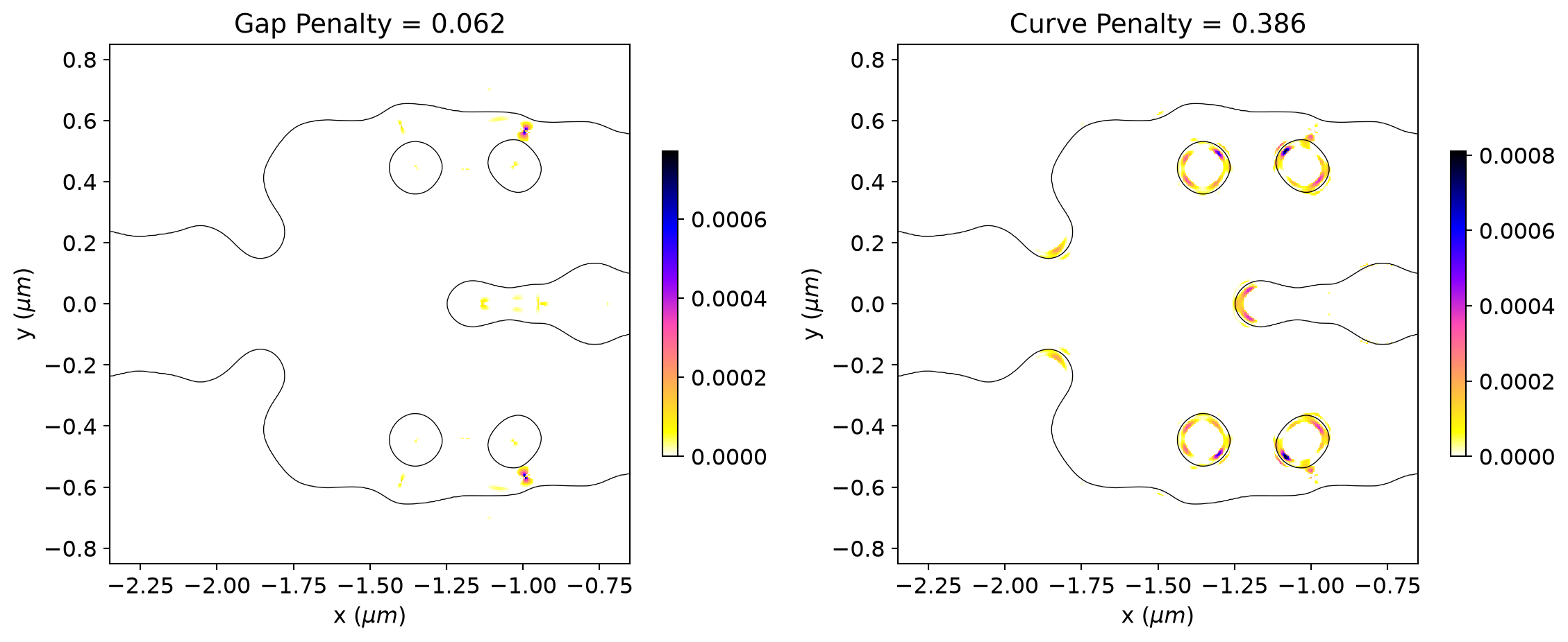
Once the inverse design is complete, we can visualize the field distributions and the wavelength dependent insertion loss.
sim_final = make_adjoint_sim(mirror_param(final_par), unfold=True)
sim_final = sim_final.copy(update=dict(monitors=(field_xy, fom_final_1)))

sim_data_final = web.run(sim_final, task_name="inv_des_final")
21:16:05 UTC Created task 'inv_des_final' with resource_id 'fdve-5ece1566-38d7-410a-beea-d59aead753fb' and task_type 'FDTD'.
             View task using web UI at
             'https://tidy3d.simulation.cloud/workbench?taskId=fdve-5ece1566-38d
             7-410a-beea-d59aead753fb'.
Task folder: 'default'.
21:16:07 UTC Estimated FlexCredit cost: 0.025. This assumes the FDTD solver runs
             for the full simulation time; if early shutoff is reached, the
             billed cost can be lower. Use 'web.real_cost(task_id)' to get the
             billed FlexCredit cost after a simulation run.
21:16:08 UTC status = queued
             To cancel the simulation, use 'web.abort(task_id)' or
             'web.delete(task_id)' or abort/delete the task in the web UI.
             Terminating the Python script will not stop the job running on the
             cloud.
21:16:16 UTC status = preprocess
21:16:20 UTC starting up solver
21:16:21 UTC running solver
21:16:26 UTC early shutoff detected at 57%, exiting.
status = postprocess
21:16:29 UTC status = success
21:16:31 UTC View simulation result at
             'https://tidy3d.simulation.cloud/workbench?taskId=fdve-5ece1566-38d
             7-410a-beea-d59aead753fb'.
21:16:32 UTC Loading results from simulation_data.hdf5
The resulting structure shows good performance, presenting insertion loss of only 0.1 dB near the central wavelength.
mode_amps = sim_data_final["out_1"]
coeffs_f = mode_amps.amps.sel(direction="+")
power_1 = np.abs(coeffs_f.sel(mode_index=0)) ** 2
power_1_db = -10 * np.log10(2 * power_1)

f, ax = plt.subplots(2, 2, figsize=(12, 10), tight_layout=True)
sim_final.plot_eps(z=0, source_alpha=0, monitor_alpha=0, ax=ax[0, 1])
ax[1, 0].plot(wl_range, power_1_db, "-k")
ax[1, 0].set_xlabel("Wavelength (um)")
ax[1, 0].set_ylabel("Power (dB)")
ax[1, 0].set_ylim(0, 4)
ax[1, 0].set_xlim(wl - bw / 2, wl + bw / 2)
ax[1, 0].set_title("Insertion Loss")
sim_data_final.plot_field("field_xy", "E", "abs^2", z=0, ax=ax[1, 1])
ax[0, 0].plot(obj_vals, "ko", label="objective")
ax[0, 0].plot(eta1_vals, "bo", label="p_1")
ax[0, 0].plot(pen_gap_vals, "ro", label="gap")
ax[0, 0].plot(pen_curve_vals, "gs", label="curvature")
ax[0, 0].set_xlabel("iterations")
ax[0, 0].set_ylabel("objective function")
ax[0, 0].legend()
ax[0, 0].set_yscale("log")
ax[0, 0].set_title(f"Final Objective Function Value: {obj_vals[-1]:.3f}")
plt.show()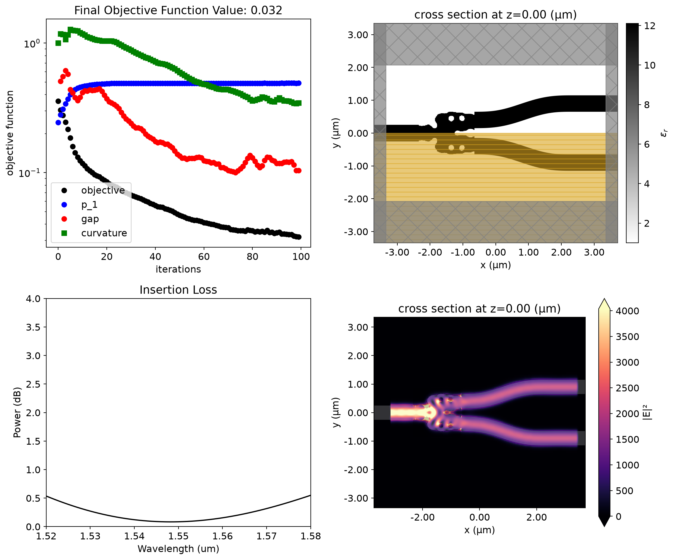
Export to GDS
The Simulation object has the .to_gds_file convenience function to export the final design to a GDS file. In addition to a file name, it is necessary to set a cross-sectional plane (z = 0 in this case) on which to evaluate the geometry, a frequency to evaluate the permittivity, and a permittivity_threshold to define the shape boundaries in custom mediums. See the GDS export notebook for a detailed example on using .to_gds_file and other GDS related functions.
sim_final.to_gds_file(
    fname="./misc/inv_des_ybranch.gds",
    z=0,
    permittivity_threshold=(eps_max + eps_min) / 2,
    frequency=freq,
)


 TERMS & CONDITIONS


 How the process works:
 Try this real URL to see an example: