





# Standard python imports.
import pickle
from typing import List

import autograd.numpy as anp
import matplotlib.pylab as plt
import numpy as np

# Import regular tidy3d.
import tidy3d as td
import tidy3d.web as web
from tidy3d.plugins.autograd import (
    adam,
    apply_updates,
    make_erosion_dilation_penalty,
    make_filter_and_project,
    value_and_grad,
)
TIDY3D
LEARNING CENTER
Example Library

Adjoint inverse design of a quantum emitter light extractor
The cost of running the entire optimization is about 8 FlexCredit (check this)
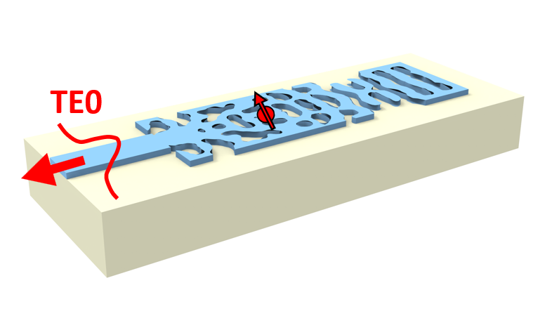
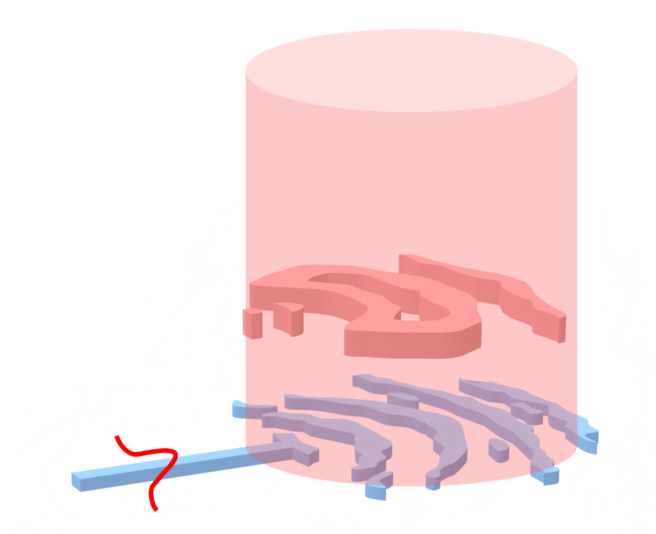
In this tutorial, we will show how to perform the adjoint-based inverse design of a quantum emitter (QE) light extraction structure. We will use a PointDipole to model the QE embedded within an integrated dielectric waveguide. Then, we will build an optimization problem to maximize the extraction efficiency of the dipole radiation into a collection waveguide. In addition, we will show how to use FluxMonitor objects in adjoint simulations to calculate the flux radiated from the dipole. You can also find helpful information in this related notebook.
If you are unfamiliar with inverse design, we recommend the inverse design lectures and this introductory tutorial.
Let’s start by importing the Python libraries used throughout this notebook.
Simulation Set Up
The coupling region (design region) extends a single-mode dielectric waveguide placed over a lower refractive index substrate. The QE is modeled as a PointDipole oriented in the y-direction. The QE is placed within the design region so we surround it with a constant refractive index region to protect it from etching.
# Geometric parameters.
cr_w = 1.0  # Coupling region width (um).
cr_l = 3.0  # Coupling region length (um).
wg_thick = 0.19  # Collection waveguide thickness (um).
wg_width = 0.35  # Collection waveguide width (um).
wg_length = 1.0  # Collection waveguide length (um).

# Material.
n_wg = 3.50  # Structure refractive index.
n_sub = 1.44  # Substrate refractive index.

# Fabrication constraints.
min_feature = 0.06  # Minimum feature size.
non_etch_r = 0.06  # Non-etched circular region radius (um).

# Inverse design set up parameters.
grid_size = 0.015  # Simulation grid size on design region (um).
max_iter = 100  # Maximum number of iterations.
iter_steps = 5  # Beta is increased at each iter_steps.
beta_min = 1.0  # Minimum value for the tanh projection parameter.
learning_rate = 0.02

# Simulation wavelength.
wl = 0.94  # Central simulation wavelength (um).
bw = 0.04  # Simulation bandwidth (um).
n_wl = 41  # Number of wavelength points within the bandwidth.
Let’s calculate some variables used throughout the notebook. Here, we will also define the QE position and monitor planes.
# Minimum and maximum values of the permittivity.
eps_max = n_wg**2
eps_min = 1.0

# Material definition.
mat_wg = td.Medium(permittivity=eps_max)
mat_sub = td.Medium(permittivity=n_sub**2)

# Wavelengths and frequencies.
wl_max = wl + bw / 2
wl_min = wl - bw / 2
wl_range = np.linspace(wl_min, wl_max, n_wl)
freq = td.C_0 / wl
freqs = td.C_0 / wl_range
freqw = 0.5 * (freqs[0] - freqs[-1])
run_time = 3e-12

# Computational domain size.
pml_spacing = 0.6 * wl
size_x = wg_length + cr_l + pml_spacing
size_y = cr_w + 2 * pml_spacing
size_z = wg_thick + 2 * pml_spacing
eff_inf = 10

# Source position and monitor planes.
cr_center_x = wg_length + cr_l / 2
qe_pos = td.Box(center=(cr_center_x - 0.5, 0, 0), size=(0, 0, 0))
qe_flux_box = td.Box(center=(cr_center_x, 0, 0), size=(cr_l, cr_w, 2 * wg_thick))
wg_mode_plan = td.Box(center=(wl / 4, 0, 0), size=(0, 4 * wg_width, 5 * wg_thick))

# Number of points on design grid.
nx_grid = int(cr_l / grid_size)
ny_grid = int(cr_w / grid_size / 2)

# xy coordinates of design grid.
x_grid = np.linspace(cr_center_x - cr_l / 2, cr_center_x + cr_l / 2, nx_grid)
y_grid = np.linspace(0, cr_w / 2, ny_grid)
Optimization Set Up
We will start defining the density-based optimization functions to transform the design parameters into permittivity values. Here we include the ConicFilter, where we impose a minimum feature size fabrication constraint, and the tangent hyperbolic projection function, eliminating intermediary permittivity values as we increase the projection parameter beta. You can find more information in the Inverse design optimization of a compact grating coupler.
def pre_process(params, beta):
    filter_project = make_filter_and_project(
        radius=min_feature, dl=grid_size, beta=beta, eta=0.5, filter_type="conic"
    )
    params1 = filter_project(params, beta)
    return params1


def get_eps(params, beta: float = 1.00):
    """Returns the permittivities after filter and projection transformations"""
    params1 = pre_process(params, beta=beta)
    eps = eps_min + (eps_max - eps_min) * params1
    eps = anp.maximum(eps, eps_min)
    eps = anp.minimum(eps, eps_max)
    return eps
This function includes a circular region of constant permittivity value surrounding the QE. The objective here is to protect the QE from etching. In applications such as single photon sources, a larger unperturbed region surrounding the QE can be helpful to reduce linewidth broadening, as stated in J. Liu, K. Konthasinghe, M. Davanco, J. Lawall, V. Anant, V. Verma, R. Mirin, S. Nam, S. Woo, D. Jin, B. Ma, Z. Chen, H. Ni, Z. Niu, K. Srinivasan, "Single Self-Assembled InAs/GaAs Quantum Dots in Photonic Nanostructures: The Role of Nanofabrication," Phys. Rev. Appl. 9(6), 064019 (2018) DOI: 10.1103/PhysRevApplied.9.064019.
def include_constant_regions(eps, circ_center=[0, 0], circ_radius=1.0):
    # Build the geometric mask.
    yv, xv = anp.meshgrid(y_grid, x_grid)

    # Shouldn't this be --> |x-x0|^2 + |y-y0|^2 <= r*2
    geo_mask = (
        anp.where(
            anp.abs((xv - circ_center[0]) ** 2 + (yv - circ_center[1]) ** 2) <= (circ_radius**2),
            1,
            0,
        )
        * eps_max
    )
    eps = anp.maximum(geo_mask, eps)
    return eps
Now, we define a function to update the td.CustomMedium using the permittivity distribution. The simulation will include mirror symmetry concerning the y-direction, so only the upper half of the design region is returned by this function during the optimization process. To get the whole structure, you need to set unfold=True.
def update_design(eps, unfold=False) -> List[td.Structure]:
    # Definition of the coordinates x,y along the design region.
    coords_x = [(cr_center_x - cr_l / 2) + ix * grid_size for ix in range(nx_grid)]
    eps_val = anp.array(eps).reshape((nx_grid, ny_grid, 1))

    if not unfold:
        coords_yp = [0 + iy * grid_size for iy in range(ny_grid)]
        coords = dict(x=coords_x, y=coords_yp, z=[0])
        eps1 = td.SpatialDataArray(eps_val, coords)
        eps_medium = td.CustomMedium(permittivity=eps1)
        box = td.Box(center=(cr_center_x, cr_w / 4, 0), size=(cr_l, cr_w / 2, wg_thick))
        structure = [td.Structure(geometry=box, medium=eps_medium)]

    # VJP for one of anp.copy(), anp.concatenate(), or anp.fliplr() not defined,
    # so the optimization should only be run with `unfold=False` for now
    else:
        coords_y = [-cr_w / 2 + iy * grid_size for iy in range(2 * ny_grid)]
        coords = dict(x=coords_x, y=coords_y, z=[0])
        eps1 = td.SpatialDataArray(
            anp.concatenate((anp.fliplr(anp.copy(eps_val)), eps_val), axis=1), coords
        )
        eps_medium = td.CustomMedium(permittivity=eps1)
        box = td.Box(center=(cr_center_x, 0, 0), size=(cr_l, cr_w, wg_thick))
        structure = [td.Structure(geometry=box, medium=eps_medium)]
    return structure
In the next cell, we define the output waveguide and the substrate, as well as the simulation monitors. It is worth mentioning the inclusion of a ModeMonitor in the output waveguide and a FluxMonitor box surrounding the dipole source to calculate the total radiated power.
# Input/output waveguide.
waveguide = td.Structure(
    geometry=td.Box.from_bounds(
        rmin=(-eff_inf, -wg_width / 2, -wg_thick / 2),
        rmax=(wg_length, wg_width / 2, wg_thick / 2),
    ),
    medium=mat_wg,
)

# Substrate layer.
substrate = td.Structure(
    geometry=td.Box.from_bounds(
        rmin=(-eff_inf, -eff_inf, -eff_inf), rmax=(eff_inf, eff_inf, -wg_thick / 2)
    ),
    medium=mat_sub,
)

# Point dipole source located at the center of TiO2 thin film.
dp_source = td.PointDipole(
    center=qe_pos.center,
    source_time=td.GaussianPulse(freq0=freq, fwidth=freqw),
    polarization="Ey",
)

# Mode monitor to compute the FOM.
mode_spec = td.ModeSpec(num_modes=1, target_neff=n_wg)
mode_monitor_fom = td.ModeMonitor(
    center=wg_mode_plan.center,
    size=wg_mode_plan.size,
    freqs=[freq],
    mode_spec=mode_spec,
    name="mode_monitor_fom",
)

# Flux monitor to compute the FOM.
flux_monitor_fom = td.FluxMonitor(
    center=qe_flux_box.center,
    size=qe_flux_box.size,
    freqs=[freq],
    name="flux_monitor_fom",
    enable_adjoint=True,
)

# Mode monitor to compute spectral response.
mode_spec = td.ModeSpec(num_modes=1, target_neff=n_wg)
mode_monitor = td.ModeMonitor(
    center=wg_mode_plan.center,
    size=wg_mode_plan.size,
    freqs=freqs,
    mode_spec=mode_spec,
    name="mode_monitor",
)

# Flux monitor to compute spectral response.
flux_monitor = td.FluxMonitor(
    center=qe_flux_box.center,
    size=qe_flux_box.size,
    freqs=freqs,
    name="flux_monitor",
)

# Field monitor to visualize the fields.
field_monitor_xy = td.FieldMonitor(
    center=(size_x / 2, 0, 0),
    size=(size_x, size_y, 0),
    freqs=freqs,
    name="field_xy",
)
Lastly, we have a function that receives the design parameters from the optimization algorithm and then gathers the simulation objects altogether to create a td.Simulation.
def make_adjoint_sim(param, beta: float = 1.00, unfold=False):
    eps = get_eps(param, beta)
    eps = include_constant_regions(
        eps, circ_center=[qe_pos.center[0], qe_pos.center[1]], circ_radius=non_etch_r
    )
    structure = update_design(eps, unfold=unfold)

    # Creates a uniform mesh for the design region.
    adjoint_dr_mesh = td.MeshOverrideStructure(
        geometry=td.Box(center=(cr_center_x, 0, 0), size=(cr_w, cr_l, wg_thick)),
        dl=[grid_size, grid_size, grid_size],
        enforce=True,
    )

    grid_spec = td.GridSpec.auto(
        wavelength=wl_max,
        min_steps_per_wvl=15,
        override_structures=[adjoint_dr_mesh],
    )

    return td.Simulation(
        size=[size_x, size_y, size_z],
        center=[size_x / 2, 0, 0],
        grid_spec=grid_spec,
        symmetry=(0, -1, 0),
        structures=[substrate, waveguide] + structure,
        sources=[dp_source],
        monitors=[field_monitor_xy, mode_monitor_fom, flux_monitor_fom],
        run_time=run_time,
        subpixel=True,
    )
Initial Light Extractor Structure
Let’s create a uniform initial permittivity distribution and verify if all the simulation objects are in the correct places.
init_par = np.ones((nx_grid, ny_grid)) * 0.5
init_design = make_adjoint_sim(init_par, beta=beta_min, unfold=True)

fig, (ax1, ax2) = plt.subplots(1, 2, tight_layout=True, figsize=(12, 4))
init_design.plot_eps(z=0, ax=ax1, monitor_alpha=0.0)
init_design.plot_eps(y=0, ax=ax2)
plt.show()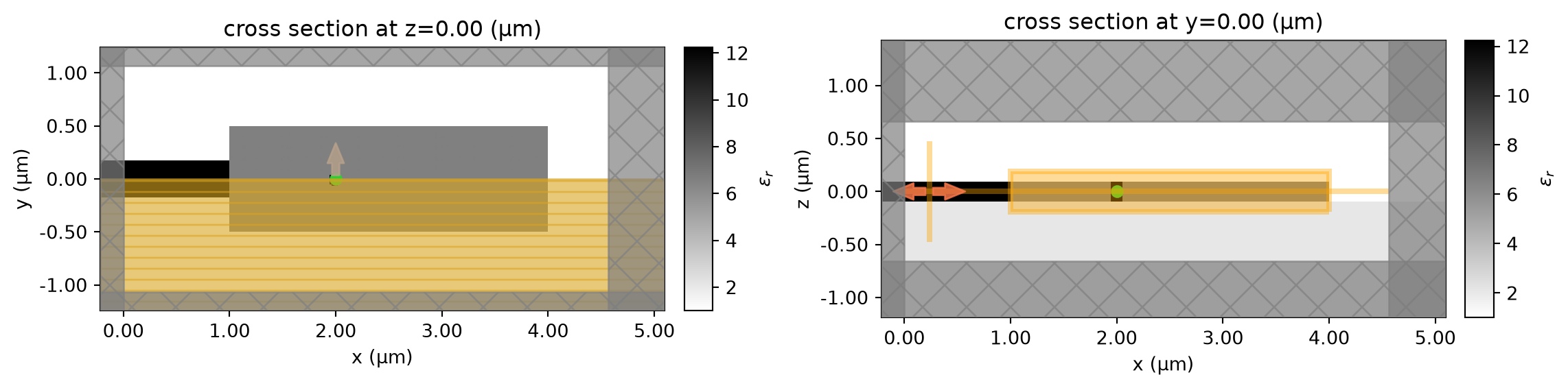
We will also look at the collection waveguide mode to ensure we have considered the correct one in the ModeMonitor setup. We use the ModeSolver plugin to calculate the first two waveguide modes, as below.
from tidy3d.plugins.mode import ModeSolver
from tidy3d.plugins.mode.web import run as run_mode_solver

sim_init = init_design.updated_copy(monitors=[field_monitor_xy, mode_monitor, flux_monitor])

mode_solver = ModeSolver(
    simulation=sim_init,
    plane=wg_mode_plan,
    mode_spec=td.ModeSpec(num_modes=2),
    freqs=[freq],
)
modes = run_mode_solver(mode_solver, reduce_simulation=True)
19:36:25 UTC Mode solver created with task_id='fdve-8f65754b-ca95-4db5-8815-3f8fe76239e9', solver_id='mo-a991b77b-25ae-4af0-920d-f77a3643893b'.
19:36:47 UTC Mode solver status: queued
19:37:09 UTC Mode solver status: running
19:37:15 UTC Mode solver status: success
After inspecting the mode field distribution, we can confirm that the fundamental waveguide mode is mainly oriented in the y-direction, thus matching the dipole orientation.
fig, axs = mode_solver.plot_field_components(
    field_names=("Ey", "Ez"),
    mode_indices=(0, 1),
    val="abs",
    f=freq,
    figsize=(10, 6),
)
for mode_ind, field_ind in np.ndindex(axs.shape):
    field_name = ("Ey", "Ez")[field_ind]
    axs[mode_ind, field_ind].set_title(f"index={mode_ind}, {field_name}(y, z)")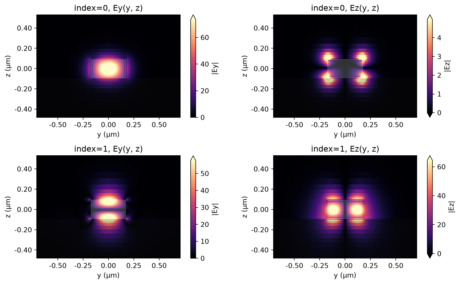
Then, we will calculate the initial coupling efficiency to see how this random structure performs.
sim_data = web.run(sim_init, task_name="initial QE light extractor (Autograd)")19:37:21 UTC Created task 'initial QE light extractor (Autograd)' with resource_id 'fdve-5f29835b-a10b-4cf2-a137-695658fabf44' and task_type 'FDTD'.
             View task using web UI at
             'https://tidy3d.simulation.cloud/workbench?taskId=fdve-5f29835b-a10
             b-4cf2-a137-695658fabf44'.
Task folder: 'default'.
19:37:23 UTC Estimated FlexCredit cost: 0.060. This assumes the FDTD solver runs
             for the full simulation time; if early shutoff is reached, the
             billed cost can be lower. Use 'web.real_cost(task_id)' to get the
             billed FlexCredit cost after a simulation run.
19:37:24 UTC status = queued
             To cancel the simulation, use 'web.abort(task_id)' or
             'web.delete(task_id)' or abort/delete the task in the web UI.
             Terminating the Python script will not stop the job running on the
             cloud.
19:37:34 UTC status = preprocess
19:37:38 UTC starting up solver
running solver
19:37:42 UTC early shutoff detected at 10%, exiting.
status = postprocess
19:37:45 UTC status = success
19:37:47 UTC View simulation result at
             'https://tidy3d.simulation.cloud/workbench?taskId=fdve-5f29835b-a10
             b-4cf2-a137-695658fabf44'.
19:37:50 UTC Loading results from simulation_data.hdf5
The modal coupling efficiency is normalized by the dipole power. That is necessary because the dipole power will likely change significantly when the optimization algorithm modifies the design region.
mode_amps = sim_data["mode_monitor"].amps.sel(direction="-", mode_index=0)
mode_power = np.abs(mode_amps) ** 2
dip_power = np.abs(sim_data["flux_monitor"].flux)

coup_eff = mode_power / dip_power

f, (ax1, ax2) = plt.subplots(1, 2, figsize=(12, 4), tight_layout=True)
ax1.plot(wl_range, coup_eff, "-k")
ax1.set_xlabel("Wavelength (um)")
ax1.set_ylabel("Coupling Efficiency")
ax1.set_ylim(0, 1)
ax1.set_xlim(wl - bw / 2, wl + bw / 2)
sim_data.plot_field("field_xy", "E", "abs^2", z=0, ax=ax2, f=freq)
plt.show()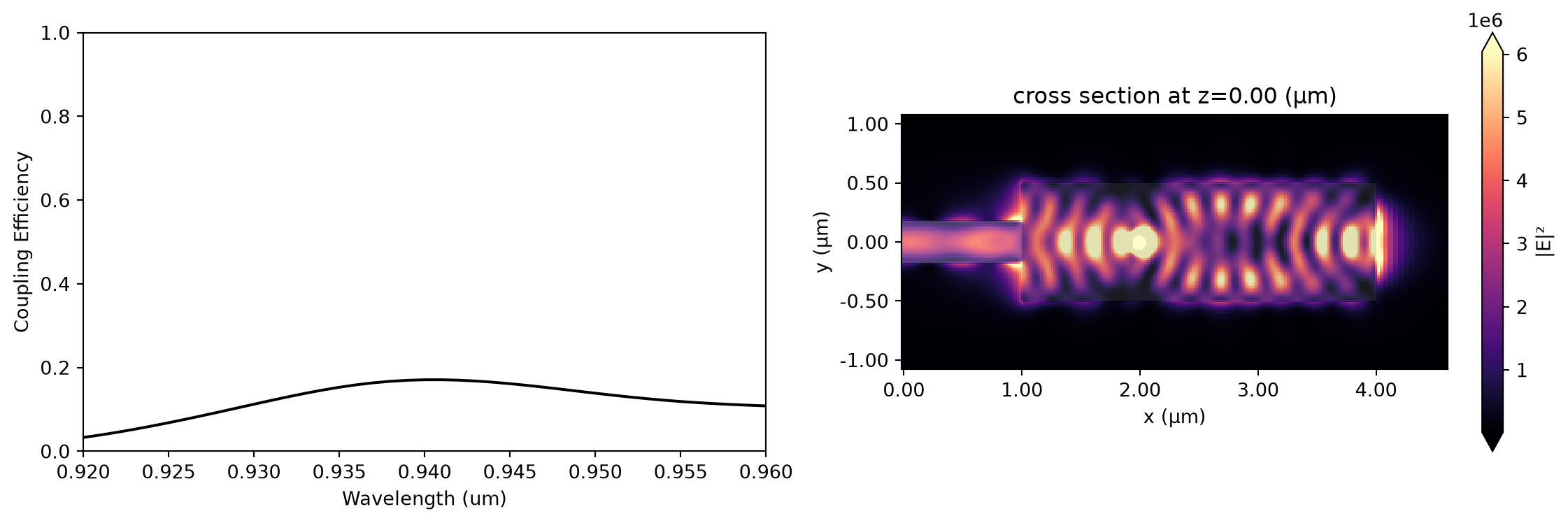
Optimization
The objective function defined next is the device figure-of-merit (FOM) minus a fabrication penalty.
# Figure of Merit (FOM) calculation.
def fom(sim_data: td.SimulationData) -> float:
    """Return the coupling efficiency."""
    # best to use autograd-wrapped numpy functions for differentiation
    mode_amps = sim_data["mode_monitor_fom"].amps.sel(direction="-", f=freq, mode_index=0).data
    mode_power = anp.sum(anp.abs(mode_amps) ** 2)

    dip_power = anp.sum(anp.abs(sim_data["flux_monitor_fom"].flux.data))

    return mode_power, dip_power


def penalty(params, beta) -> float:
    """Penalize changes in structure after erosion and dilation to enforce larger feature sizes."""
    params_processed = pre_process(params, beta=beta)
    erode_dilate_penalty = make_erosion_dilation_penalty(radius=min_feature, dl=grid_size)
    ed_penalty = erode_dilate_penalty(params_processed)
    return ed_penalty


# Objective function to be passed to the optimization algorithm.
def obj(param, beta: float = 1.0, step_num: int = None, verbose: bool = False) -> float:
    sim = make_adjoint_sim(param, beta, unfold=False)  # non-differentiable if `unfold=True`
    task_name = "inv_des"
    if step_num:
        task_name += f"_step_{step_num}"
    sim_data = web.run(sim, task_name=task_name, verbose=verbose)
    mode_power, dip_power = fom(sim_data)
    fom_val = mode_power / dip_power
    penalty_weight = 0.1
    penalty_val = penalty(param, beta)
    J = fom_val - penalty_weight * penalty_val
    return J, [sim_data, mode_power, dip_power, penalty_val]


# Function to calculate the objective function value and its gradient with respect to the design parameters.
# Use tidy3d's wrapped ag.value_and_grad() for it's auxiliary data functionality
obj_grad = value_and_grad(obj, has_aux=True)
In the following cell, we define some functions to save the optimization progress and load a previous optimization from the file.
# where to store history
history_fname = "misc/qe_light_coupler.pkl"


def save_history(history_dict: dict) -> None:
    """Convenience function to save the history to file."""
    with open(history_fname, "wb") as file:
        pickle.dump(history_dict, file)


def load_history() -> dict:
    """Convenience method to load the history from file."""
    with open(history_fname, "rb") as file:
        history_dict = pickle.load(file)
    return history_dict
Then, we will start a new optimization or load the parameters of a previous one.
# initialize adam optimizer with starting parameters
optimizer = adam(learning_rate=learning_rate)

try:
    history_dict = load_history()
    opt_state = history_dict["opt_states"][-1]
    params = history_dict["params"][-1]
    opt_state = optimizer.init(params)
    num_iters_completed = len(history_dict["params"])
    print("Loaded optimization checkpoint from file.")
    print(f"Found {num_iters_completed} iterations previously completed out of {max_iter} total.")
    if num_iters_completed < max_iter:
        print("Will resume optimization.")
    else:
        print("Optimization completed, will return results.")

except FileNotFoundError:
    params = anp.array(init_par)
    opt_state = optimizer.init(params)
    history_dict = dict(
        values=[],
        coupl_eff=[],
        penalty=[],
        params=[],
        gradients=[],
        opt_states=[opt_state],
        data=[],
        beta=[],
    )
In the optimization loop, we will gradually increase the projection parameter beta to eliminate intermediary permittivity values. At each iteration, we record the design parameters and the optimization history to restore them as needed.
iter_done = len(history_dict["values"])
if iter_done < max_iter:
    # small # of iters for quick testing
    for i in range(iter_done, max_iter):
        print(f"Iteration = ({i + 1} / {max_iter})")
        plt.subplots(1, 1, figsize=(3, 2))
        plt.imshow(np.flipud(1 - params.T), cmap="gray", vmin=0, vmax=1)
        plt.axis("off")
        plt.show()

        # Compute gradient and current objective function value.
        beta_i = i // iter_steps + beta_min
        (value, gradient), data = obj_grad(params, beta=beta_i, step_num=(i + 1))
        sim_data_i, mode_power_i, dip_power_i, penalty_val_i = [data[0]] + [
            dat._value for dat in data[1:]
        ]
        # Outputs.
        print(f"\tbeta = {beta_i}")
        print(f"\tJ = {value:.4e}")
        print(f"\tgrad_norm = {np.linalg.norm(gradient):.4e}")
        print(f"\tpenalty = {penalty_val_i:.3f}")
        print(f"\tmode power = {mode_power_i:.3f}")
        print(f"\tdip power = {dip_power_i:.3f}")
        print(f"\tcoupling efficiency = {mode_power_i / dip_power_i:.3f}")

        # Compute and apply updates to the optimizer based on gradient (-1 sign to maximize obj_fn).
        updates, opt_state = optimizer.update(-gradient, opt_state, params)
        params = apply_updates(params, updates)

        # Cap parameters between 0 and 1.
        params = anp.minimum(params, 1.0)
        params = anp.maximum(params, 0.0)

        # Save history.
        history_dict["values"].append(value)
        history_dict["coupl_eff"].append(mode_power_i / dip_power_i)
        history_dict["penalty"].append(penalty_val_i)
        history_dict["params"].append(params)
        history_dict["beta"].append(beta_i)
        history_dict["gradients"].append(gradient)
        history_dict["opt_states"].append(opt_state)
        # history_dict["data"].append(sim_data_i)  # Uncomment to store data, can create large files.
        save_history(history_dict)
Iteration = (1 / 100)
    beta = 1.0
    J = 7.1427e-02
    grad_norm = 6.3862e-02
    penalty = 1.000
    mode power = 473.637
    dip power = 2762.899
    coupling efficiency = 0.171
Iteration = (2 / 100)
    beta = 1.0
    J = 2.3237e-01
    grad_norm = 6.6931e-02
    penalty = 1.000
    mode power = 1006.721
    dip power = 3028.948
    coupling efficiency = 0.332
Iteration = (3 / 100)
    beta = 1.0
    J = 3.8047e-01
    grad_norm = 6.0493e-02
    penalty = 1.000
    mode power = 1504.393
    dip power = 3131.087
    coupling efficiency = 0.480
Iteration = (4 / 100)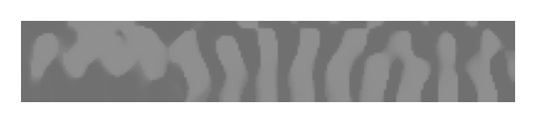
    beta = 1.0
    J = 5.0013e-01
    grad_norm = 5.2723e-02
    penalty = 1.000
    mode power = 1981.499
    dip power = 3301.765
    coupling efficiency = 0.600
Iteration = (5 / 100)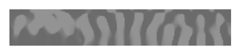
    beta = 1.0
    J = 5.9371e-01
    grad_norm = 4.3683e-02
    penalty = 1.000
    mode power = 2490.432
    dip power = 3590.031
    coupling efficiency = 0.694
Iteration = (6 / 100)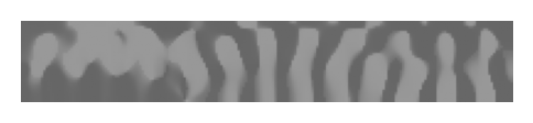
    beta = 2.0
    J = 6.9714e-01
    grad_norm = 5.0917e-02
    penalty = 1.000
    mode power = 3180.133
    dip power = 3989.418
    coupling efficiency = 0.797
Iteration = (7 / 100)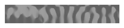
    beta = 2.0
    J = 7.4126e-01
    grad_norm = 3.5748e-02
    penalty = 1.000
    mode power = 3869.043
    dip power = 4599.094
    coupling efficiency = 0.841
Iteration = (8 / 100)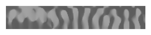
    beta = 2.0
    J = 7.7145e-01
    grad_norm = 2.8583e-02
    penalty = 1.000
    mode power = 4554.618
    dip power = 5226.471
    coupling efficiency = 0.871
Iteration = (9 / 100)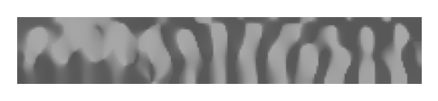
    beta = 2.0
    J = 7.9287e-01
    grad_norm = 2.7701e-02
    penalty = 1.000
    mode power = 5232.111
    dip power = 5859.924
    coupling efficiency = 0.893
Iteration = (10 / 100)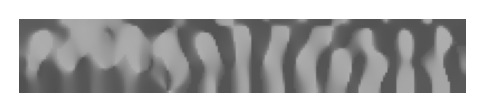
    beta = 2.0
    J = 8.0951e-01
    grad_norm = 2.6579e-02
    penalty = 1.000
    mode power = 6080.603
    dip power = 6685.595
    coupling efficiency = 0.910
Iteration = (11 / 100)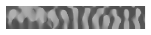
    beta = 3.0
    J = 8.0209e-01
    grad_norm = 7.6534e-02
    penalty = 1.000
    mode power = 7495.064
    dip power = 8308.865
    coupling efficiency = 0.902
Iteration = (12 / 100)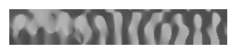
    beta = 3.0
    J = 8.3183e-01
    grad_norm = 3.5587e-02
    penalty = 0.999
    mode power = 9206.108
    dip power = 9880.194
    coupling efficiency = 0.932
Iteration = (13 / 100)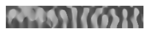
    beta = 3.0
    J = 8.3035e-01
    grad_norm = 4.7137e-02
    penalty = 0.999
    mode power = 10448.820
    dip power = 11232.179
    coupling efficiency = 0.930
Iteration = (14 / 100)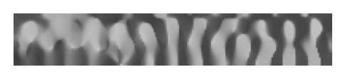
    beta = 3.0
    J = 8.2096e-01
    grad_norm = 7.9938e-02
    penalty = 0.999
    mode power = 10235.078
    dip power = 11115.192
    coupling efficiency = 0.921
Iteration = (15 / 100)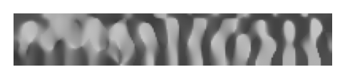
    beta = 3.0
    J = 8.3270e-01
    grad_norm = 6.9472e-02
    penalty = 0.998
    mode power = 9589.003
    dip power = 10283.176
    coupling efficiency = 0.932
Iteration = (16 / 100)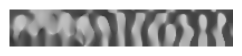
    beta = 4.0
    J = 8.0078e-01
    grad_norm = 1.6094e-01
    penalty = 0.984
    mode power = 8125.545
    dip power = 9036.899
    coupling efficiency = 0.899
Iteration = (17 / 100)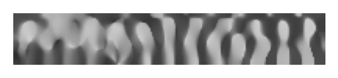
    beta = 4.0
    J = 8.4291e-01
    grad_norm = 7.1355e-02
    penalty = 0.979
    mode power = 10514.818
    dip power = 11176.390
    coupling efficiency = 0.941
Iteration = (18 / 100)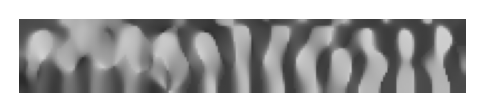
    beta = 4.0
    J = 8.5404e-01
    grad_norm = 4.8601e-02
    penalty = 0.973
    mode power = 13731.098
    dip power = 14433.069
    coupling efficiency = 0.951
Iteration = (19 / 100)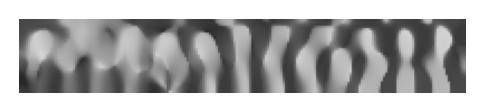
    beta = 4.0
    J = 8.4766e-01
    grad_norm = 7.5401e-02
    penalty = 0.967
    mode power = 16405.052
    dip power = 17371.467
    coupling efficiency = 0.944
Iteration = (20 / 100)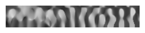
    beta = 4.0
    J = 8.5402e-01
    grad_norm = 6.5638e-02
    penalty = 0.961
    mode power = 17898.337
    dip power = 18838.477
    coupling efficiency = 0.950
Iteration = (21 / 100)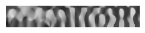
    beta = 5.0
    J = 8.6521e-01
    grad_norm = 7.8295e-02
    penalty = 0.886
    mode power = 18974.513
    dip power = 19892.689
    coupling efficiency = 0.954
Iteration = (22 / 100)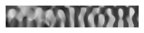
    beta = 5.0
    J = 8.7045e-01
    grad_norm = 6.6717e-02
    penalty = 0.876
    mode power = 18614.565
    dip power = 19429.129
    coupling efficiency = 0.958
Iteration = (23 / 100)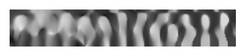
    beta = 5.0
    J = 8.7768e-01
    grad_norm = 3.4743e-02
    penalty = 0.866
    mode power = 14847.319
    dip power = 15397.035
    coupling efficiency = 0.964
Iteration = (24 / 100)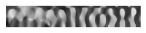
    beta = 5.0
    J = 8.7735e-01
    grad_norm = 4.5013e-02
    penalty = 0.856
    mode power = 10924.360
    dip power = 11344.803
    coupling efficiency = 0.963
Iteration = (25 / 100)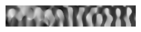
    beta = 5.0
    J = 8.7782e-01
    grad_norm = 6.2367e-02
    penalty = 0.845
    mode power = 10057.548
    dip power = 10450.800
    coupling efficiency = 0.962
Iteration = (26 / 100)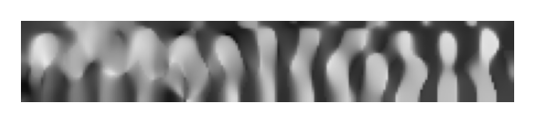
    beta = 6.0
    J = 8.8279e-01
    grad_norm = 7.3759e-02
    penalty = 0.748
    mode power = 9926.287
    dip power = 10366.473
    coupling efficiency = 0.958
Iteration = (27 / 100)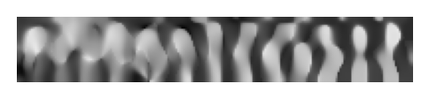
    beta = 6.0
    J = 8.9116e-01
    grad_norm = 5.2254e-02
    penalty = 0.737
    mode power = 15331.134
    dip power = 15889.521
    coupling efficiency = 0.965
Iteration = (28 / 100)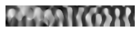
    beta = 6.0
    J = 8.9903e-01
    grad_norm = 5.1621e-02
    penalty = 0.726
    mode power = 22832.098
    dip power = 23497.572
    coupling efficiency = 0.972
Iteration = (29 / 100)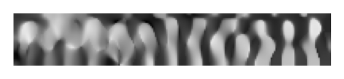
    beta = 6.0
    J = 9.0250e-01
    grad_norm = 7.5577e-02
    penalty = 0.717
    mode power = 25718.239
    dip power = 26400.492
    coupling efficiency = 0.974
Iteration = (30 / 100)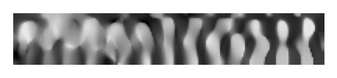
    beta = 6.0
    J = 9.0259e-01
    grad_norm = 4.7752e-02
    penalty = 0.708
    mode power = 23974.983
    dip power = 24631.490
    coupling efficiency = 0.973
Iteration = (31 / 100)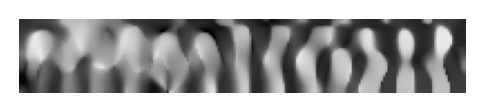
    beta = 7.0
    J = 8.9788e-01
    grad_norm = 1.0700e-01
    penalty = 0.623
    mode power = 13120.206
    dip power = 13664.062
    coupling efficiency = 0.960
Iteration = (32 / 100)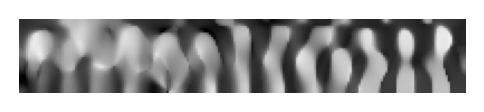
    beta = 7.0
    J = 9.0605e-01
    grad_norm = 6.3559e-02
    penalty = 0.617
    mode power = 13590.802
    dip power = 14043.976
    coupling efficiency = 0.968
Iteration = (33 / 100)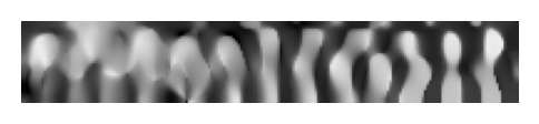
    beta = 7.0
    J = 9.0947e-01
    grad_norm = 4.8678e-02
    penalty = 0.611
    mode power = 17326.758
    dip power = 17852.377
    coupling efficiency = 0.971
Iteration = (34 / 100)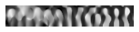
    beta = 7.0
    J = 9.0847e-01
    grad_norm = 6.6275e-02
    penalty = 0.605
    mode power = 21434.099
    dip power = 22119.561
    coupling efficiency = 0.969
Iteration = (35 / 100)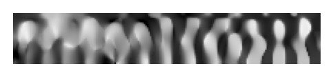
    beta = 7.0
    J = 9.0785e-01
    grad_norm = 6.6433e-02
    penalty = 0.600
    mode power = 22842.104
    dip power = 23600.205
    coupling efficiency = 0.968
Iteration = (36 / 100)
    beta = 8.0
    J = 9.0063e-01
    grad_norm = 1.3711e-01
    penalty = 0.539
    mode power = 15743.467
    dip power = 16494.039
    coupling efficiency = 0.954
Iteration = (37 / 100)
    beta = 8.0
    J = 9.1841e-01
    grad_norm = 2.6427e-02
    penalty = 0.534
    mode power = 23328.318
    dip power = 24005.031
    coupling efficiency = 0.972
Iteration = (38 / 100)
    beta = 8.0
    J = 9.1356e-01
    grad_norm = 1.2956e-01
    penalty = 0.529
    mode power = 29832.356
    dip power = 30866.090
    coupling efficiency = 0.967
Iteration = (39 / 100)
    beta = 8.0
    J = 9.1678e-01
    grad_norm = 9.8895e-02
    penalty = 0.525
    mode power = 25597.249
    dip power = 26408.865
    coupling efficiency = 0.969
Iteration = (40 / 100)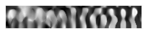
    beta = 8.0
    J = 9.2318e-01
    grad_norm = 7.7721e-02
    penalty = 0.521
    mode power = 18071.358
    dip power = 18530.287
    coupling efficiency = 0.975
Iteration = (41 / 100)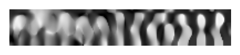
    beta = 9.0
    J = 9.1634e-01
    grad_norm = 1.8407e-01
    penalty = 0.472
    mode power = 11702.458
    dip power = 12145.066
    coupling efficiency = 0.964
Iteration = (42 / 100)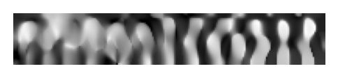
    beta = 9.0
    J = 9.2311e-01
    grad_norm = 1.0598e-01
    penalty = 0.468
    mode power = 20545.367
    dip power = 21181.959
    coupling efficiency = 0.970
Iteration = (43 / 100)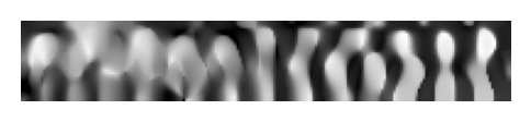
    beta = 9.0
    J = 9.2187e-01
    grad_norm = 1.6990e-01
    penalty = 0.465
    mode power = 33026.187
    dip power = 34105.926
    coupling efficiency = 0.968
Iteration = (44 / 100)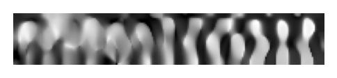
    beta = 9.0
    J = 9.3207e-01
    grad_norm = 9.4006e-02
    penalty = 0.461
    mode power = 31134.252
    dip power = 31829.051
    coupling efficiency = 0.978
Iteration = (45 / 100)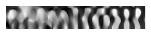
    beta = 9.0
    J = 9.2140e-01
    grad_norm = 1.5419e-01
    penalty = 0.457
    mode power = 20009.688
    dip power = 20689.457
    coupling efficiency = 0.967
Iteration = (46 / 100)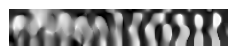
    beta = 10.0
    J = 9.2274e-01
    grad_norm = 2.0090e-01
    penalty = 0.420
    mode power = 12803.053
    dip power = 13271.484
    coupling efficiency = 0.965
Iteration = (47 / 100)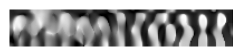
    beta = 10.0
    J = 9.3463e-01
    grad_norm = 8.5038e-02
    penalty = 0.417
    mode power = 25599.519
    dip power = 26221.092
    coupling efficiency = 0.976
Iteration = (48 / 100)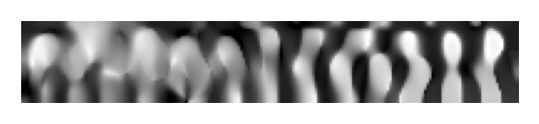
    beta = 10.0
    J = 9.2303e-01
    grad_norm = 2.5730e-01
    penalty = 0.414
    mode power = 46624.615
    dip power = 48344.336
    coupling efficiency = 0.964
Iteration = (49 / 100)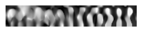
    beta = 10.0
    J = 9.3555e-01
    grad_norm = 7.6268e-02
    penalty = 0.411
    mode power = 29958.936
    dip power = 30676.455
    coupling efficiency = 0.977
Iteration = (50 / 100)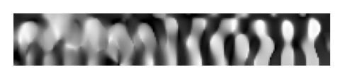
    beta = 10.0
    J = 9.3742e-01
    grad_norm = 1.3022e-01
    penalty = 0.407
    mode power = 15537.793
    dip power = 15885.174
    coupling efficiency = 0.978
Iteration = (51 / 100)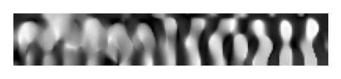
    beta = 11.0
    J = 9.2486e-01
    grad_norm = 2.2858e-01
    penalty = 0.377
    mode power = 9204.664
    dip power = 9562.306
    coupling efficiency = 0.963
Iteration = (52 / 100)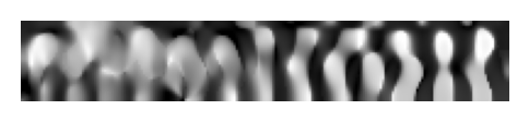
    beta = 11.0
    J = 9.4329e-01
    grad_norm = 7.6061e-02
    penalty = 0.374
    mode power = 19935.578
    dip power = 20328.195
    coupling efficiency = 0.981
Iteration = (53 / 100)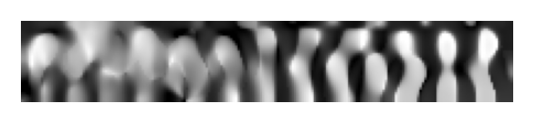
    beta = 11.0
    J = 9.3610e-01
    grad_norm = 3.0954e-01
    penalty = 0.371
    mode power = 61081.357
    dip power = 62766.551
    coupling efficiency = 0.973
Iteration = (54 / 100)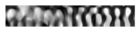
    beta = 11.0
    J = 9.3954e-01
    grad_norm = 1.1333e-01
    penalty = 0.366
    mode power = 32199.770
    dip power = 32986.406
    coupling efficiency = 0.976
Iteration = (55 / 100)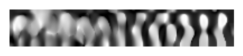
    beta = 11.0
    J = 9.4723e-01
    grad_norm = 8.7204e-02
    penalty = 0.362
    mode power = 15169.928
    dip power = 15425.603
    coupling efficiency = 0.983
Iteration = (56 / 100)
    beta = 12.0
    J = 9.4329e-01
    grad_norm = 1.6728e-01
    penalty = 0.338
    mode power = 8518.089
    dip power = 8717.407
    coupling efficiency = 0.977
Iteration = (57 / 100)
    beta = 12.0
    J = 9.4479e-01
    grad_norm = 1.5326e-01
    penalty = 0.336
    mode power = 12587.848
    dip power = 12866.322
    coupling efficiency = 0.978
Iteration = (58 / 100)
    beta = 12.0
    J = 9.4748e-01
    grad_norm = 8.2549e-02
    penalty = 0.333
    mode power = 31391.334
    dip power = 32006.426
    coupling efficiency = 0.981
Iteration = (59 / 100)
    beta = 12.0
    J = 9.4183e-01
    grad_norm = 3.8975e-01
    penalty = 0.331
    mode power = 76294.427
    dip power = 78258.805
    coupling efficiency = 0.975
Iteration = (60 / 100)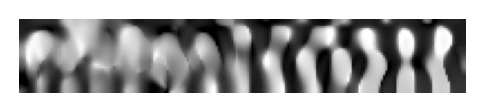
    beta = 12.0
    J = 9.5113e-01
    grad_norm = 1.0414e-01
    penalty = 0.328
    mode power = 23941.104
    dip power = 24332.824
    coupling efficiency = 0.984
Iteration = (61 / 100)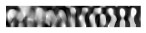
    beta = 13.0
    J = 9.4807e-01
    grad_norm = 1.5746e-01
    penalty = 0.309
    mode power = 8215.002
    dip power = 8391.254
    coupling efficiency = 0.979
Iteration = (62 / 100)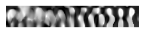
    beta = 13.0
    J = 9.4126e-01
    grad_norm = 2.2533e-01
    penalty = 0.307
    mode power = 7798.941
    dip power = 8024.197
    coupling efficiency = 0.972
Iteration = (63 / 100)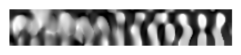
    beta = 13.0
    J = 9.5221e-01
    grad_norm = 1.6412e-01
    penalty = 0.304
    mode power = 10705.064
    dip power = 10894.683
    coupling efficiency = 0.983
Iteration = (64 / 100)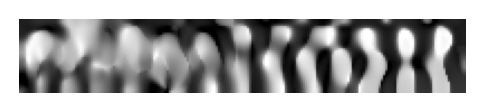
    beta = 13.0
    J = 9.5325e-01
    grad_norm = 6.0898e-02
    penalty = 0.301
    mode power = 28331.966
    dip power = 28810.357
    coupling efficiency = 0.983
Iteration = (65 / 100)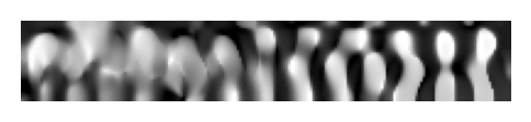
    beta = 13.0
    J = 9.4628e-01
    grad_norm = 4.0561e-01
    penalty = 0.299
    mode power = 81034.465
    dip power = 83013.711
    coupling efficiency = 0.976
Iteration = (66 / 100)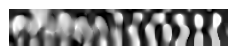
    beta = 14.0
    J = 9.4575e-01
    grad_norm = 3.2084e-01
    penalty = 0.282
    mode power = 19989.570
    dip power = 20523.795
    coupling efficiency = 0.974
Iteration = (67 / 100)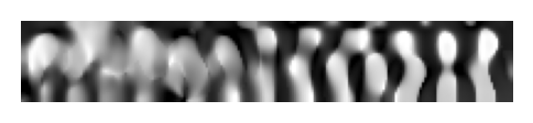
    beta = 14.0
    J = 9.5336e-01
    grad_norm = 1.4801e-01
    penalty = 0.280
    mode power = 16612.344
    dip power = 16928.156
    coupling efficiency = 0.981
Iteration = (68 / 100)
    beta = 14.0
    J = 9.4567e-01
    grad_norm = 3.0256e-01
    penalty = 0.277
    mode power = 20717.463
    dip power = 21283.432
    coupling efficiency = 0.973
Iteration = (69 / 100)
    beta = 14.0
    J = 9.5832e-01
    grad_norm = 1.2265e-01
    penalty = 0.274
    mode power = 28308.840
    dip power = 28717.668
    coupling efficiency = 0.986
Iteration = (70 / 100)
    beta = 14.0
    J = 9.5064e-01
    grad_norm = 2.3618e-01
    penalty = 0.272
    mode power = 53504.638
    dip power = 54717.863
    coupling efficiency = 0.978
Iteration = (71 / 100)
    beta = 15.0
    J = 9.5897e-01
    grad_norm = 1.1757e-01
    penalty = 0.259
    mode power = 57507.422
    dip power = 58389.977
    coupling efficiency = 0.985
Iteration = (72 / 100)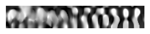
    beta = 15.0
    J = 9.5485e-01
    grad_norm = 2.2342e-01
    penalty = 0.257
    mode power = 52085.003
    dip power = 53115.672
    coupling efficiency = 0.981
Iteration = (73 / 100)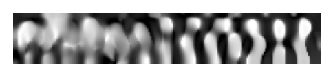
    beta = 15.0
    J = 9.5972e-01
    grad_norm = 1.3436e-01
    penalty = 0.255
    mode power = 30666.387
    dip power = 31125.539
    coupling efficiency = 0.985
Iteration = (74 / 100)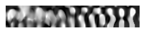
    beta = 15.0
    J = 9.6006e-01
    grad_norm = 1.6465e-01
    penalty = 0.254
    mode power = 28415.311
    dip power = 28835.992
    coupling efficiency = 0.985
Iteration = (75 / 100)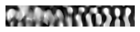
    beta = 15.0
    J = 9.5651e-01
    grad_norm = 1.8701e-01
    penalty = 0.252
    mode power = 44835.278
    dip power = 45670.129
    coupling efficiency = 0.982
Iteration = (76 / 100)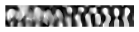
    beta = 16.0
    J = 9.6197e-01
    grad_norm = 3.7146e-02
    penalty = 0.241
    mode power = 39260.429
    dip power = 39813.836
    coupling efficiency = 0.986
Iteration = (77 / 100)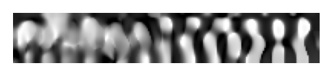
    beta = 16.0
    J = 9.5658e-01
    grad_norm = 1.8358e-01
    penalty = 0.239
    mode power = 54897.302
    dip power = 55987.762
    coupling efficiency = 0.981
Iteration = (78 / 100)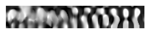
    beta = 16.0
    J = 9.6049e-01
    grad_norm = 2.1517e-01
    penalty = 0.238
    mode power = 74340.396
    dip power = 75530.219
    coupling efficiency = 0.984
Iteration = (79 / 100)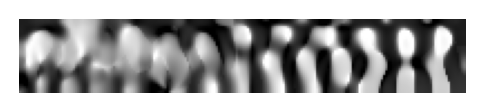
    beta = 16.0
    J = 9.6269e-01
    grad_norm = 9.0773e-02
    penalty = 0.235
    mode power = 29286.055
    dip power = 29695.393
    coupling efficiency = 0.986
Iteration = (80 / 100)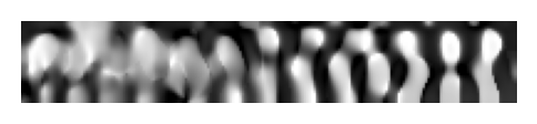
    beta = 16.0
    J = 9.5864e-01
    grad_norm = 1.5802e-01
    penalty = 0.233
    mode power = 21789.253
    dip power = 22190.566
    coupling efficiency = 0.982
Iteration = (81 / 100)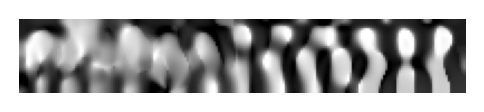
    beta = 17.0
    J = 9.5906e-01
    grad_norm = 1.4991e-01
    penalty = 0.222
    mode power = 24998.311
    dip power = 25474.828
    coupling efficiency = 0.981
Iteration = (82 / 100)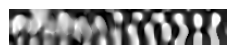
    beta = 17.0
    J = 9.5866e-01
    grad_norm = 2.7292e-01
    penalty = 0.220
    mode power = 83470.653
    dip power = 85119.992
    coupling efficiency = 0.981
Iteration = (83 / 100)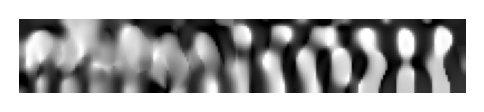
    beta = 17.0
    J = 9.5643e-01
    grad_norm = 2.9625e-01
    penalty = 0.217
    mode power = 43940.506
    dip power = 44921.684
    coupling efficiency = 0.978
Iteration = (84 / 100)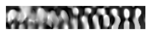
    beta = 17.0
    J = 9.5449e-01
    grad_norm = 2.7986e-01
    penalty = 0.215
    mode power = 26020.569
    dip power = 26660.217
    coupling efficiency = 0.976
Iteration = (85 / 100)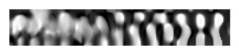
    beta = 17.0
    J = 9.5983e-01
    grad_norm = 1.7246e-01
    penalty = 0.213
    mode power = 25213.187
    dip power = 25697.502
    coupling efficiency = 0.981
Iteration = (86 / 100)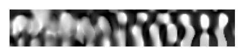
    beta = 18.0
    J = 9.6083e-01
    grad_norm = 1.9436e-01
    penalty = 0.205
    mode power = 39548.374
    dip power = 40300.621
    coupling efficiency = 0.981
Iteration = (87 / 100)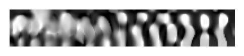
    beta = 18.0
    J = 9.5985e-01
    grad_norm = 4.9640e-01
    penalty = 0.203
    mode power = 105236.710
    dip power = 107365.422
    coupling efficiency = 0.980
Iteration = (88 / 100)
    beta = 18.0
    J = 9.5037e-01
    grad_norm = 4.4681e-01
    penalty = 0.202
    mode power = 14128.312
    dip power = 14556.350
    coupling efficiency = 0.971
Iteration = (89 / 100)
    beta = 18.0
    J = 9.5163e-01
    grad_norm = 3.3728e-01
    penalty = 0.201
    mode power = 12594.293
    dip power = 12960.915
    coupling efficiency = 0.972
Iteration = (90 / 100)
    beta = 18.0
    J = 9.6086e-01
    grad_norm = 1.4232e-01
    penalty = 0.200
    mode power = 17499.077
    dip power = 17841.375
    coupling efficiency = 0.981
Iteration = (91 / 100)
    beta = 19.0
    J = 9.5418e-01
    grad_norm = 3.6515e-01
    penalty = 0.193
    mode power = 25912.466
    dip power = 26617.756
    coupling efficiency = 0.974
Iteration = (92 / 100)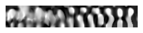
    beta = 19.0
    J = 9.5338e-01
    grad_norm = 1.2997e+00
    penalty = 0.191
    mode power = 176533.393
    dip power = 181522.109
    coupling efficiency = 0.973
Iteration = (93 / 100)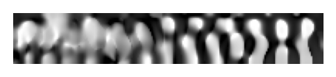
    beta = 19.0
    J = 9.3338e-01
    grad_norm = 6.1480e-01
    penalty = 0.192
    mode power = 5742.912
    dip power = 6029.058
    coupling efficiency = 0.953
Iteration = (94 / 100)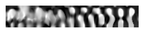
    beta = 19.0
    J = 9.0977e-01
    grad_norm = 4.2404e-01
    penalty = 0.191
    mode power = 2756.794
    dip power = 2967.904
    coupling efficiency = 0.929
Iteration = (95 / 100)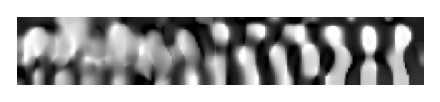
    beta = 19.0
    J = 9.0232e-01
    grad_norm = 5.2855e-01
    penalty = 0.190
    mode power = 2408.596
    dip power = 2614.218
    coupling efficiency = 0.921
Iteration = (96 / 100)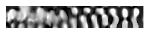
    beta = 20.0
    J = 9.2989e-01
    grad_norm = 2.9412e-01
    penalty = 0.186
    mode power = 2228.995
    dip power = 2350.151
    coupling efficiency = 0.948
Iteration = (97 / 100)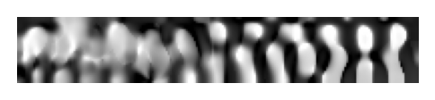
    beta = 20.0
    J = 9.2500e-01
    grad_norm = 6.0745e-01
    penalty = 0.185
    mode power = 2439.442
    dip power = 2585.547
    coupling efficiency = 0.943
Iteration = (98 / 100)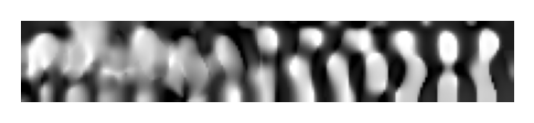
    beta = 20.0
    J = 9.4166e-01
    grad_norm = 2.0362e-01
    penalty = 0.183
    mode power = 3735.461
    dip power = 3891.078
    coupling efficiency = 0.960
Iteration = (99 / 100)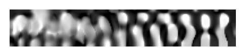
    beta = 20.0
    J = 9.2847e-01
    grad_norm = 3.8854e-01
    penalty = 0.181
    mode power = 6116.362
    dip power = 6461.295
    coupling efficiency = 0.947
Iteration = (100 / 100)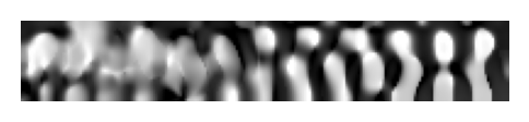
    beta = 20.0
    J = 9.4033e-01
    grad_norm = 1.3126e-01
    penalty = 0.179
    mode power = 8888.252
    dip power = 9275.336
    coupling efficiency = 0.958
Ultimately, we get all the information to assess the optimization results.
obj_vals = np.array(history_dict["values"])
ce_vals = np.array(history_dict["coupl_eff"])
pen_vals = np.array(history_dict["penalty"])
final_par_density = history_dict["params"][-1]
final_beta = history_dict["beta"][-1]
# just to inspect design at different iterations
def unfold_params(params):
params = np.concatenate((np.fliplr(np.copy(params)), params), axis=1)
return params
params1 = history_dict["params"][32]
params1_full = pre_process(params1, beta=final_beta)
params1_full = include_constant_regions(
params1_full, circ_center=[qe_pos.center[0], qe_pos.center[1]], circ_radius=non_etch_r
)
params1_full = unfold_params(params1_full)
params2 = history_dict["params"][-1]
params2_full = pre_process(params2, beta=final_beta)
params2_full = include_constant_regions(
params2_full, circ_center=[qe_pos.center[0], qe_pos.center[1]], circ_radius=non_etch_r
)
params2_full = unfold_params(params2_full)plt.imshow(
1 - np.flipud(params1_full.T),
cmap="gray",
vmin=0,
vmax=1,
extent=[wg_length, cr_l + wg_length, -cr_w / 2, cr_w / 2],
)
plt.plot(dp_source.center[0], 0, "r*")
plt.show()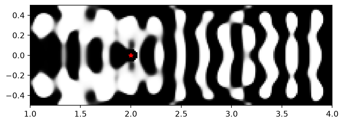
plt.imshow(
    1 - np.flipud(params2_full.T),
    cmap="gray",
    vmin=0,
    vmax=1,
    extent=[wg_length, cr_l + wg_length, -cr_w / 2, cr_w / 2],
)
plt.plot(dp_source.center[0], 0, "r*")
plt.show()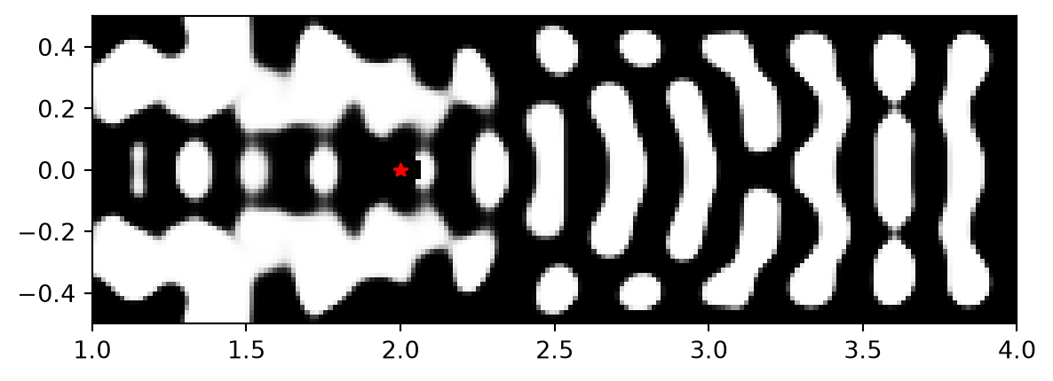
Results
The following figure shows how coupling efficiency and the fabrication penalty have evolved along the optimization process. The coupling efficiency quickly rises above 0.8, and along the binarization process, we can observe two large drops before a more stable final optimization stage. The formation of resonant modes sensitive to the small structural changes can potentially explain this behavior. The discontinuities in the fabrication penalty curve are caused by the increments in the projection parameter beta at each 5 iterations.
fig, ax = plt.subplots(1, 1, figsize=(7, 5))
ax.plot(ce_vals, "ko", label="C. Efficiency")
ax.plot(pen_vals, "bs", label="Fab. Penalty")
ax.plot(history_dict["values"], "ro", label="J")
ax.set_xlabel("iterations")
ax.set_ylabel("objective function")
ax.set_title(f"Final Coupling Efficiency: {ce_vals[-1]:.2f}")
ax.axvline(x=32, color="r", linestyle="--")

ax.legend()
plt.show()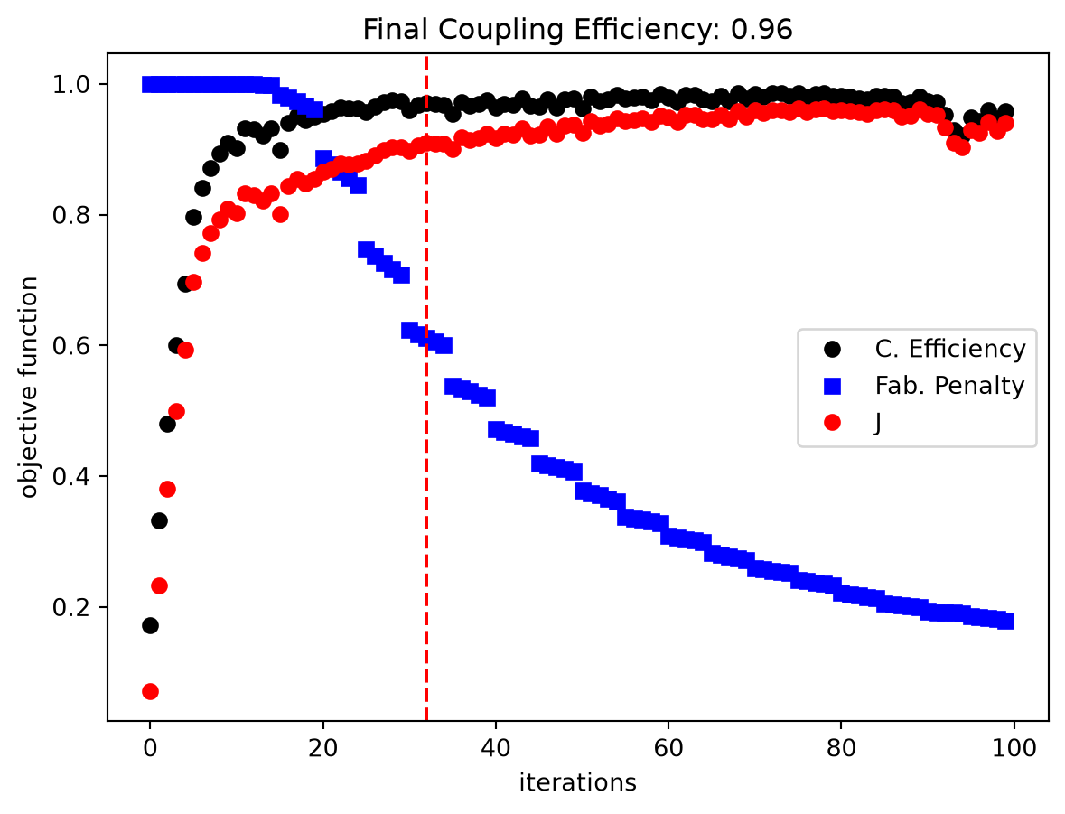
Interestingly, fully binarizing the design from iteration 32 produced a device with great coupling efficiency (~97%), but minimal purcell enhancement
plt.plot([np.linalg.norm(grad) for grad in history_dict["gradients"]])
plt.ylabel("norm(grad)")
plt.xlabel("iteration")
Text(0.5, 0, 'iteration')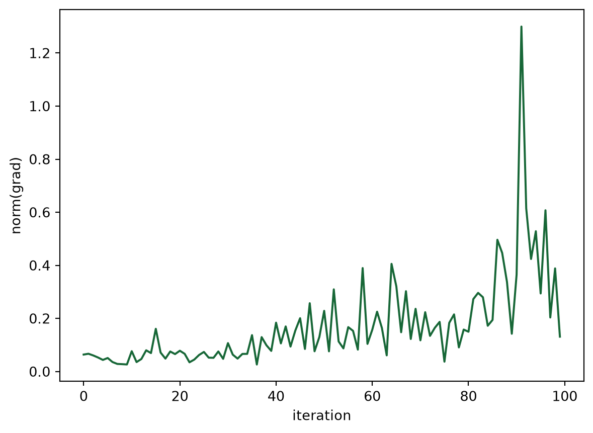
Makes a nice animation of the design parameters and gradient evolution during the optimization
import matplotlib.animation as animation
from mpl_toolkits.axes_grid1 import make_axes_locatable

fig, axs = plt.subplots(nrows=2, ncols=1)

gradients = history_dict["gradients"]
params = history_dict["params"]
gradients = [unfold_params(grad).T for grad in gradients]
params = [unfold_params(init_par).T] + [unfold_params(1.0 - p).T for p in params]

div = make_axes_locatable(axs[1])
div0 = make_axes_locatable(axs[0])
cax = div.append_axes("top", size="5%", pad=0.05)
cax0 = div0.append_axes("bottom", size="5%", pad=0.05)
cax0.axis("off")


def animate(i):
    im_g = axs[1].imshow(
        gradients[i], interpolation="none", vmin=np.min(gradients[i]), vmax=np.max(gradients[i])
    )
    axs[0].imshow(params[i], interpolation="none", cmap="gray", vmin=0, vmax=1)
    axs[1].axis("off")
    axs[0].axis("off")
    cax.cla()
    fig.colorbar(im_g, cax=cax, orientation="horizontal").ax.xaxis.set_ticks_position("top")

    axs[0].set_title(f"iteration {i}")


anim = animation.FuncAnimation(
    fig, animate, frames=len(history_dict["params"]), blit=False, interval=500
)
anim.save("autograd_anim.mp4", fps=2.0)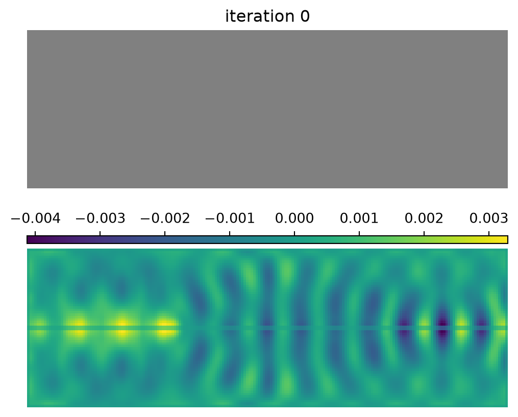
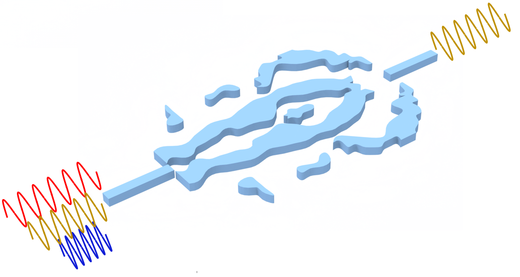
Interestingly, the final quantum emitter light extractor resembles a nanocavity, even though we have considered only the coupling efficiency into the output waveguide in the optimization. We have DBR mirrors on both sides of the dipole. However, on the left side, the mirror has only a few periods and partially reflects the radiation, which couples to the output waveguide.
# here, removing substrate improved performance, but also blue-shifted cavity resonance a bit.

fig, ax = plt.subplots(1, figsize=(10, 4))
# Substrate layer.
substrate = td.Structure(
    geometry=td.Box.from_bounds(
        rmin=(-eff_inf, -eff_inf, -eff_inf), rmax=(eff_inf, eff_inf, -wg_thick / 2)
    ),
    medium=td.Medium(permittivity=1.0),
)
sim_final = make_adjoint_sim(params2, beta=final_beta, unfold=True)
sim_final = sim_final.updated_copy(monitors=[field_monitor_xy, mode_monitor, flux_monitor])
sim_final.plot_eps(
    z=0,
    source_alpha=0,
    monitor_alpha=0,
    ax=ax,
)
plt.show()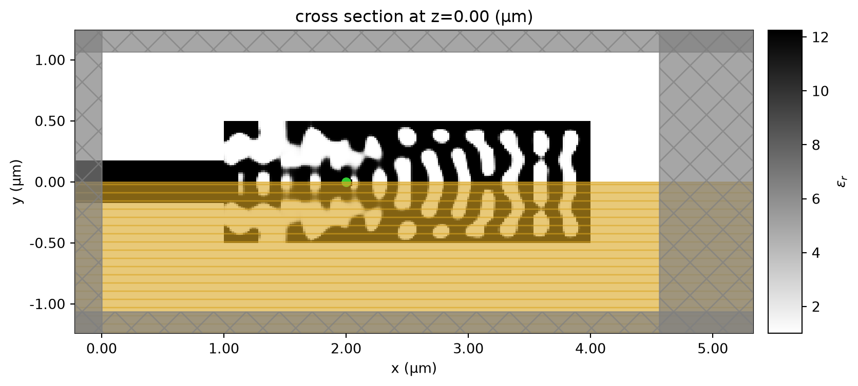
To better understand the resultant design, let’s simulate the final structure to obtain its spectral response and field distribution.
sim_data_final = web.run(sim_final, task_name="final QE light extractor")23:03:17 UTC Created task 'final QE light extractor' with resource_id 'fdve-7158aa53-229e-4930-858a-eea3fc20abca' and task_type 'FDTD'.
             View task using web UI at
             'https://tidy3d.simulation.cloud/workbench?taskId=fdve-7158aa53-229
             e-4930-858a-eea3fc20abca'.
Task folder: 'default'.
23:03:19 UTC Estimated FlexCredit cost: 0.057. This assumes the FDTD solver runs
             for the full simulation time; if early shutoff is reached, the
             billed cost can be lower. Use 'web.real_cost(task_id)' to get the
             billed FlexCredit cost after a simulation run.
23:03:20 UTC status = queued
             To cancel the simulation, use 'web.abort(task_id)' or
             'web.delete(task_id)' or abort/delete the task in the web UI.
             Terminating the Python script will not stop the job running on the
             cloud.
23:03:37 UTC starting up solver
running solver
23:03:54 UTC early shutoff detected at 33%, exiting.
status = postprocess
23:03:59 UTC status = success
23:04:01 UTC View simulation result at
             'https://tidy3d.simulation.cloud/workbench?taskId=fdve-7158aa53-229
             e-4930-858a-eea3fc20abca'.
23:04:06 UTC Loading results from simulation_data.hdf5
In this cavity-like system, the extraction efficiency of photons from the QE into the collection waveguide mode is proportional to \(\beta\times C_{wg}\), where the \(\beta\)-factor quantifies the fraction of the QE spontaneous emission emitted in the cavity mode, and \(C_{wg}\) is the fraction of the cavity photons coupled to the guided mode A. Enderlin, Y. Ota, R. Ohta, N. Kumagai, S. Ishida, S. Iwamoto, and Y. Arakawa, "High guided mode–cavity mode coupling for an efficient extraction of spontaneous emission of a single quantum dot embedded in a photonic crystal nanobeam cavity," Phys. Rev. B 86, 075314 (2012) DOI: 10.1103/PhysRevB.86.075314. By the field distribution image below, we can see a cavity mode resonance, which should increase the Purcell factor at the QE position, thus contributing to a higher \(\beta\)-factor. At the same time, the partial reflection mirror at the left side was potentially optimized to adjust \(C_{wg}\).
f, ax1 = plt.subplots(1, 1, figsize=(12, 4), tight_layout=True)
sim_data_final.plot_field("field_xy", "E", "abs^2", z=0, ax=ax1, f=freqs[0])
plt.show()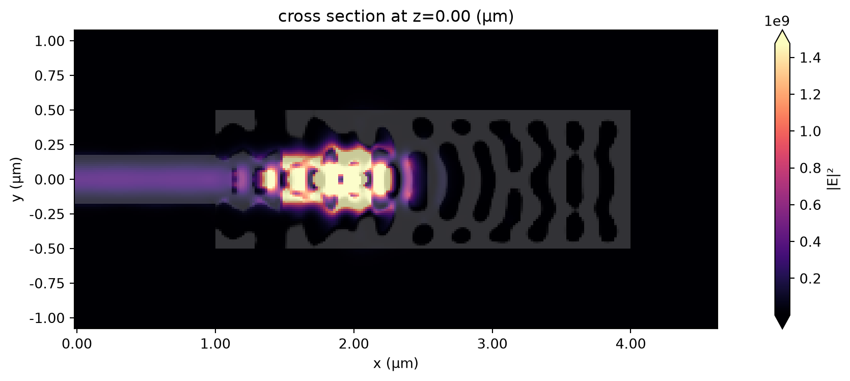
To conclude, we will calculate the final coupling efficiency and the cavity Purcell value. The coupling efficiency is above 80% along an extensive wavelength range, and we have confirmed the Purcell enhancement.
# Coupling efficiency.
mode_amps = sim_data_final["mode_monitor"].amps.sel(direction="-", mode_index=0)
mode_power = np.abs(mode_amps) ** 2
dip_power = np.abs(sim_data_final["flux_monitor"].flux)
coup_eff = mode_power / dip_power

# Purcell factor.
bulk_power = ((2 * np.pi * freqs) ** 2 / (12 * np.pi)) * (td.MU_0 * n_wg / td.C_0)
bulk_power = bulk_power * 2 ** (2 * np.sum(np.abs(sim_final.symmetry)))
purcell = dip_power / bulk_power

f, (ax1, ax2) = plt.subplots(1, 2, figsize=(10, 4), tight_layout=True)
ax1.plot(wl_range, coup_eff, "-k")
ax1.set_xlabel("Wavelength (um)")
ax1.set_ylabel("Coupling Efficiency")
ax1.set_ylim(0, 1)
ax1.set_xlim(wl - bw / 2, wl + bw / 2)
ax2.plot(wl_range, purcell, "-k")
ax2.set_xlabel("Wavelength (um)")
ax2.set_ylabel("Purcell Factor")
ax2.set_xlim(wl - bw / 2, wl + bw / 2)
plt.show()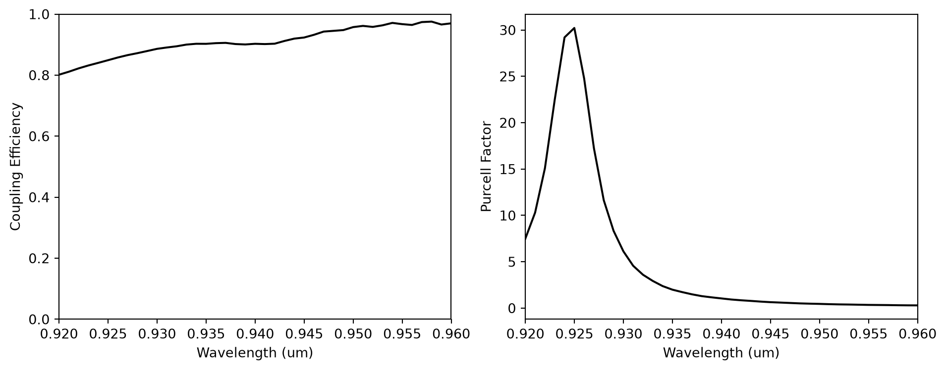
print(np.max(coup_eff.values))
print(np.min(coup_eff.values))
0.9754737614849407
0.8013754449981956Export to GDS
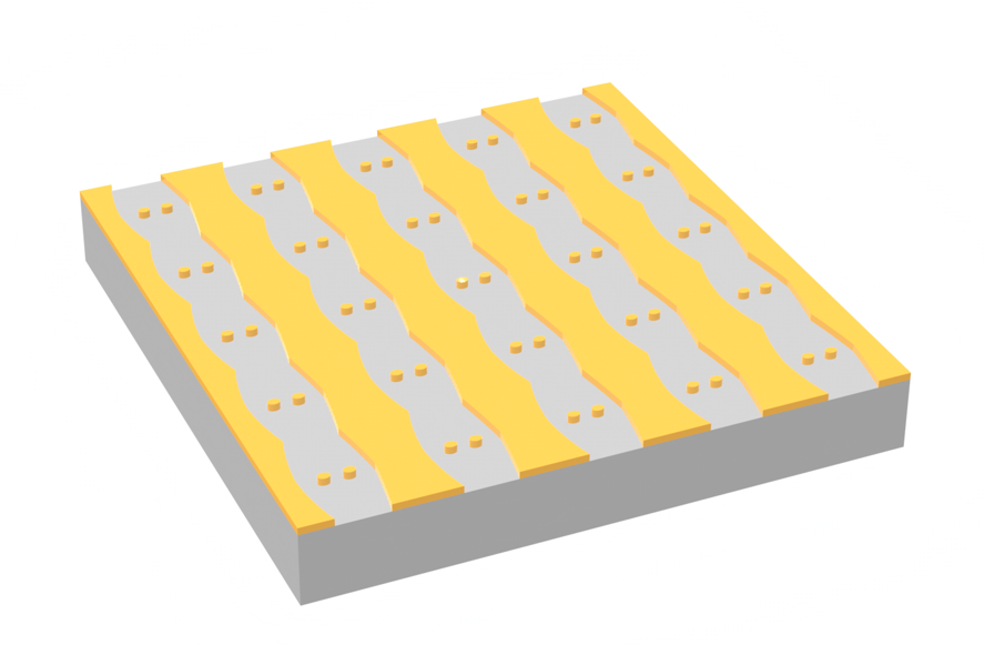
The Simulation object has the .to_gds_file convenience function to export the final design to a GDS file. In addition to a file name, it is necessary to set a cross-sectional plane (z = 0 in this case) on which to evaluate the geometry, a frequency to evaluate the permittivity, and a permittivity_threshold to define the shape boundaries in custom mediums. See the GDS export notebook for a detailed example on using .to_gds_file and other GDS related functions.
# make the misc/ directory to store the GDS file if it doesn't exist already
import os

if not os.path.exists("./misc/"):
    os.mkdir("./misc/")

sim_final.to_gds_file(
    fname="./misc/inv_des_light_extractor_autograd.gds",
    z=0,
    permittivity_threshold=(eps_max + eps_min) / 2,
    frequency=freq,
)


 TERMS & CONDITIONS


 How the process works:
 Try this real URL to see an example: