





# Standard python imports.
from typing import List

# Import autograd to be able to use automatic differentiation.
import autograd.numpy as anp
import matplotlib.pylab as plt
import numpy as np
import scipy as sp

# Import regular tidy3d.
import tidy3d as td
import tidy3d.web as web
from autograd import value_and_grad
TIDY3D
LEARNING CENTER
Example Library

Inverse design optimization of a compact grating coupler
This notebook contains a long optimization. Running the entire notebook will cost about 10 FlexCredits and take a few hours.
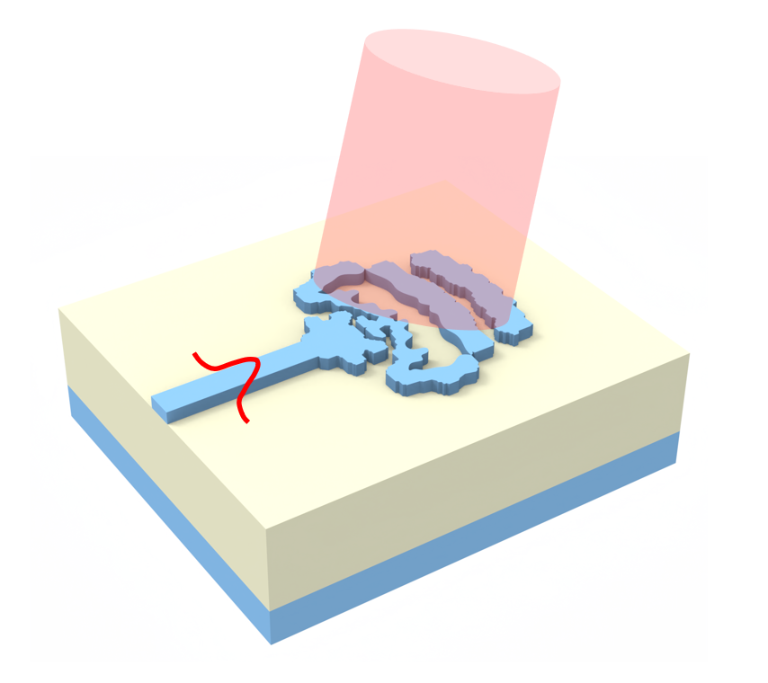
The ability to couple light in and out of photonic integrated circuits (PICs) is crucial for developing wafer-scale systems and tests. This need makes designing efficient and compact grating couplers an important task in the PIC development cycle. In this notebook, we will demonstrate how to use tidy3d to perform the inverse design of a compact 3D grating coupler. We will show how to improve design fabricability by enhancing permittivity binarization and controlling the device’s minimum feature size.
In addition, if you are interested in more conventional designs, we modeled an uniform grating coupler and a Focusing apodized grating coupler in previous case studies. For more integrated photonic examples, please visit our examples page. If you are new to the finite-difference time-domain (FDTD) method, we highly recommend going through our FDTD101 tutorials. FDTD simulations can diverge due to various reasons. If you run into any simulation divergence issues, please follow the steps outlined in our troubleshooting guide to resolve it.
We start by importing our typical python packages, plus autograd and tidy3d.
Grating Coupler Inverse Design Configuration
The grating coupler inverse design begins with a rectangular design region connected to a \(Si\) waveguide. Throughout the optimization process, this initial structure evolves to convert a vertically incident Gaussian-like mode from an optical fiber into a guided mode and then funnel it into the \(Si\) waveguide.
We are considering a full-etched grating structure, so a \(SiO_{2}\) BOX layer is included. To reduce backreflection, we adjusted the fiber tilt angle to \(10^{\circ}\) [1, 2].
In the following block of code, you can find the parameters that can be modified to configure the grating coupler structure, optimization, and simulation setup. Special care should be devoted to the it_per_step and opt_steps variables below.
# Geometric parameters.
w_thick = 0.22  # Waveguide thickness (um).
w_width = 0.5  # Waveguide width (um).
w_length = 1.0  # Waveguide length (um).
box_thick = 1.6  # SiO2 BOX thickness (um).
spot_size = 2.5  # Spot size of the input Gaussian field regarding a lensed fiber (um).
fiber_tilt = 10.0  # Fiber tilt angle (degrees).
src_offset = 0.05  # Distance between the source focus and device (um).

# Material.
nSi = 3.48  # Silicon refractive index.
nSiO2 = 1.44  # Silica refractive index.

# Design region parameters.
gc_width = 4.0  # Grating coupler width (um).
gc_length = 4.0  # Grating coupler length (um).
dr_grid_size = 0.02  # Grid size within the design region (um).

# Inverse design setup parameters.
#################################################################
# Total number of iterations = opt_steps x it_per_step.
it_per_step = 1  # Number of iterations per optimization step.
opt_steps = 75  # Number of optimization steps.
#################################################################
eta = 0.50  # Threshold value for the projection filter.
fom_name = "fom_field"  # Name of the monitor used to compute the objective function.

# Simulation wavelength.
wl = 1.55  # Central simulation wavelength (um).
bw = 0.06  # Simulation bandwidth (um).
n_wl = 61  # Number of wavelength points within the bandwidth.

# feature size
min_feature_size = 0.080
filter_radius = min_feature_size

# Buffer layer thickness
border_buffer = 0.16

# projection
beta_min = 1.0
beta_max = 30.0
total_iter = opt_steps * it_per_step
print(f"Total iterations = {total_iter}")Total iterations = 75Inverse Design Optimization Set Up
We will calculate the values of some parameters used throughout the inverse design set up.
# Minimum and maximum values for the permittivities.
eps_max = nSi**2
eps_min = 1.0

# Material definitions.
mat_si = td.Medium(permittivity=eps_max)  # Waveguide material.
mat_sio2 = td.Medium(permittivity=nSiO2**2)  # Substrate material.

# Wavelengths and frequencies.
wl_max = wl + bw / 2
wl_min = wl - bw / 2
wl_range = np.linspace(wl_min, wl_max, n_wl)
freq = td.C_0 / wl
freqs = td.C_0 / wl_range
freqw = 0.5 * (freqs[0] - freqs[-1])
run_time = 5e-12

# Computational domain size.
pml_spacing = 0.6 * wl
size_x = pml_spacing + w_length + gc_length + 2 * border_buffer
size_y = gc_width + 2 * pml_spacing + 2 * border_buffer
size_z = w_thick + box_thick + 2 * pml_spacing
center_z = size_z / 2 - pml_spacing - w_thick / 2
eff_inf = 1000

# Inverse design variables.
src_pos_z = w_thick / 2 + src_offset
mon_pos_x = -size_x / 2 + 0.25 * wl
mon_w = int(3 * w_width / dr_grid_size) * dr_grid_size
mon_h = int(5 * w_thick / dr_grid_size) * dr_grid_size
nx = int((gc_length + 2 * border_buffer) / dr_grid_size)
ny = int((gc_width + 2 * border_buffer) / dr_grid_size / 2.0)
npar = int(nx * ny)
dr_size_x = nx * dr_grid_size
dr_size_y = 2 * ny * dr_grid_size
dr_center_x = -size_x / 2 + w_length + dr_size_x / 2
n_border = int(border_buffer / dr_grid_size)
First, we will introduce the simulation components that do not change during optimization, such as the \(Si\) waveguide and \(SiO_{2}\) BOX layer. Additionally, we will include a Gaussian source to drive the simulations, and a mode monitor to compute the objective function.
# Input/output waveguide.
waveguide = td.Structure(
    geometry=td.Box.from_bounds(
        rmin=(-eff_inf, -w_width / 2, -w_thick / 2),
        rmax=(-size_x / 2 + w_length, w_width / 2, w_thick / 2),
    ),
    medium=mat_si,
)

# SiO2 BOX layer.
sio2_substrate = td.Structure(
    geometry=td.Box.from_bounds(
        rmin=(-eff_inf, -eff_inf, -w_thick / 2 - box_thick),
        rmax=(eff_inf, eff_inf, -w_thick / 2),
    ),
    medium=mat_sio2,
)

# Si substrate.
si_substrate = td.Structure(
    geometry=td.Box.from_bounds(
        rmin=(-eff_inf, -eff_inf, -eff_inf),
        rmax=(eff_inf, eff_inf, -w_thick / 2 - box_thick),
    ),
    medium=mat_si,
)

# Gaussian source focused above the grating coupler.
gauss_source = td.GaussianBeam(
    center=(dr_center_x, 0, src_pos_z),
    size=(dr_size_x - 2 * border_buffer, dr_size_y - 2 * border_buffer, 0),
    source_time=td.GaussianPulse(freq0=freq, fwidth=freqw),
    pol_angle=np.pi / 2,
    angle_theta=fiber_tilt * np.pi / 180.0,
    direction="-",
    num_freqs=7,
    waist_radius=spot_size / 2,
)

# Monitor where we will compute the objective function from.
mode_spec = td.ModeSpec(num_modes=1, target_neff=nSi)
fom_monitor = td.ModeMonitor(
    center=[mon_pos_x, 0, 0],
    size=[0, mon_w, mon_h],
    freqs=[freq],
    mode_spec=mode_spec,
    name=fom_name,
)
Now, we will define a random vector of initial design parameters or load a previously designed structure.
Note: if a previous optimization file is found, the optimizer will pick up where that left off instead.
init_par = np.random.uniform(0, 1, int(npar))
init_par = sp.ndimage.gaussian_filter(init_par, 1)
init_par = init_par.reshape((nx, ny))
Fabrication Constraints
We will use the tidy3d.plugins.autograd plugin to introduce functions that improve device fabricability. A classical conic density filter, which is popular in topology optimization problems, is used to enforce a minimum feature size specified by the filter_radius variable. Next, a hyperbolic tangent projection function is applied to eliminate grayscale and obtain a binarized permittivity pattern. The beta parameter controls the sharpness of the transition in the projection function, and for better results, this parameter should be gradually increased throughout the optimization process. Finally, the design parameters are transformed into permittivity values. For a detailed review of these methods, refer to [3].
We will also introduce a buffer layer around the design region to enhance fabricability at the interfaces. The permittivity is enforced to lower values within the buffer layer, except at the output waveguide connection where we want a smooth transition.
def get_eps(design_param: np.ndarray, beta: float = 1.00, binarize: bool = False) -> np.ndarray:
    """Returns the permittivities after applying a conic density filter on design parameters
    to enforce fabrication constraints, followed by a binarization projection function
    which reduces grayscale.
    Parameters:
        design_param: np.ndarray
            Vector of design parameters.
        beta: float = 1.0
            Sharpness parameter for the projection filter.
        binarize: bool = False
            Enforce binarization.
    Returns:
        eps: np.ndarray
            Permittivity vector.
    """

    # Calculates the permittivities from the transformed design parameters.
    eps = get_eps_values(design_param, beta=beta)
    if binarize:
        eps = anp.where(eps < (eps_min + eps_max) / 2, eps_min, eps_max)
    else:
        eps = anp.where(eps < eps_min, eps_min, eps)
        eps = anp.where(eps > eps_max, eps_max, eps)
    return eps
from tidy3d.plugins.autograd import make_filter_and_project, rescale
filter_project = make_filter_and_project(filter_radius, dr_grid_size, padding="constant")
def interface_buffer(params):
"""Introduce a buffer around design to enhance fabricability at the interfaces."""
mask = anp.zeros_like(params)
mask[0:n_border, :] = 0
mask[nx - n_border :, :] = 0
mask[:, ny - n_border :] = 0
mask[0:n_border, 0 : int((w_width / 2) / dr_grid_size) + 1] = 1
return params * (1 - mask) + mask
def pre_process(params, beta):
"""Get the permittivity values (1, eps_wg) array as a function of the parameters (0,1)"""
params1 = interface_buffer(params)
params2 = filter_project(params1, beta=beta)
params3 = filter_project(params2, beta=beta)
return params3
def get_eps_values(params: np.ndarray, beta: float) -> np.ndarray:
"""Get the relative permittivity array given the parameters."""
params = pre_process(params, beta=beta)
eps_values = rescale(params, eps_min, eps_max)
return eps_valuesThe permittivity values obtained from the design parameters are then used to build a CustomMedium. As we will consider symmetry about the x-axis in the simulations, only the upper-half part of the design region needs to be populated. A Structure built using the CustomMedium will be returned by the following function:
def update_design(eps, unfold: bool = False) -> List[td.Structure]:
    """Reflects the structure about the x-axis."""
    nyii = ny
    y_min = 0
    dr_s_y = dr_size_y / 2
    dr_c_y = dr_s_y / 2
    eps_val = anp.array(eps).reshape((nx, ny, 1))
    if unfold:
        nyii = 2 * ny
        y_min = -dr_size_y / 2
        dr_s_y = dr_size_y
        dr_c_y = 0
        eps_val = anp.concatenate((anp.fliplr(anp.copy(eps_val)), eps_val), axis=1)

    # Definition of the coordinates x,y along the design region.
    coords_x = [(dr_center_x - dr_size_x / 2) + ix * dr_grid_size for ix in range(nx)]
    coords_y = [y_min + iy * dr_grid_size for iy in range(nyii)]
    coords = dict(x=coords_x, y=coords_y, z=[0])

    # Creation of a custom medium using the values of the design parameters.
    permittivity = td.SpatialDataArray(eps_val, coords=coords)
    eps_medium = td.CustomMedium(permittivity=permittivity)
    box = td.Box(center=(dr_center_x, dr_c_y, 0), size=(dr_size_x, dr_s_y, w_thick))
    design_structure = td.Structure(geometry=box, medium=eps_medium)
    return [design_structure]
Next, we will write a function to return the td.Simulation object. Note that we are using a MeshOverrideStructure to obtain a uniform mesh over the design region.
def make_adjoint_sim(
    design_param: np.ndarray,
    beta: float = 1.00,
    unfold: bool = False,
    binarize: bool = False,
) -> td.Simulation:
    # Builds the design region from the design parameters.
    eps = get_eps(design_param, beta, binarize)
    design_structure = update_design(eps, unfold=unfold)

    # Creates a uniform mesh for the design region.
    adjoint_dr_mesh = td.MeshOverrideStructure(
        geometry=td.Box(center=(dr_center_x, 0, 0), size=(dr_size_x, dr_size_y, w_thick)),
        dl=[dr_grid_size, dr_grid_size, dr_grid_size],
        enforce=True,
    )

    return td.Simulation(
        size=[size_x, size_y, size_z],
        center=[0, 0, -center_z],
        grid_spec=td.GridSpec.auto(
            wavelength=wl_max,
            min_steps_per_wvl=15,
            override_structures=[adjoint_dr_mesh],
        ),
        symmetry=(0, -1, 0),
        structures=[waveguide, sio2_substrate, si_substrate] + design_structure,
        sources=[gauss_source],
        monitors=[fom_monitor],
        run_time=run_time,
        subpixel=True,
    )
Let’s visualize the simulation set up and verify if all the elements are in their correct places.
init_design = make_adjoint_sim(init_par, beta=beta_min)

fig, (ax1, ax2) = plt.subplots(1, 2, tight_layout=True, figsize=(10, 10))
init_design.plot_eps(z=0, ax=ax1)
init_design.plot_eps(y=0, ax=ax2)
plt.show()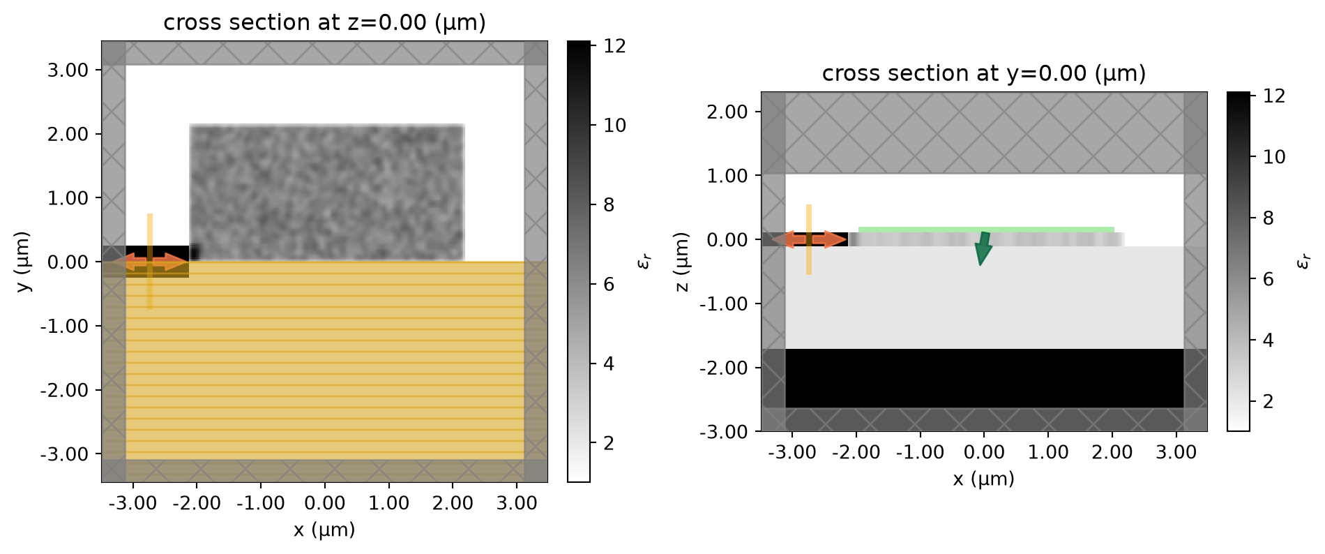
from tidy3d.plugins.autograd import make_erosion_dilation_penalty

erode_dilate_penalty = make_erosion_dilation_penalty(filter_radius, dr_grid_size)


# Figure of Merit (FOM) calculation.
def fom(sim_data: td.SimulationData) -> float:
    """Return the power at the mode index of interest."""
    output_amps = sim_data[fom_name].amps
    amp = output_amps.sel(direction="-", f=freq, mode_index=0).values
    return anp.sum(anp.abs(amp) ** 2)


def penalty(params, beta) -> float:
    """Penalty function based on amount of change in parameters after erosion and dilation."""
    params_processed = pre_process(params, beta=beta)
    return erode_dilate_penalty(params_processed)


# Objective function to be passed to the optimization algorithm.
def obj(design_param, beta: float = 1.0, step_num: int = None, verbose: bool = False) -> float:
    sim = make_adjoint_sim(design_param, beta)
    task_name = "inv_des"
    if step_num:
        task_name += f"_step_{step_num}"
    sim_data = web.run(sim, task_name=task_name, verbose=verbose)
    fom_val = fom(sim_data)
    feature_size_penalty = penalty(design_param, beta=beta)
    J = fom_val - feature_size_penalty
    return J


# Function to calculate the objective function value and its
# gradient with respect to the design parameters.
obj_grad = value_and_grad(obj)
Optimization
We need to provide an objective function and its gradients with respect to the design parameters of the optimization algorithm.
Our figure-of-merit (FOM) is the coupling efficiency of the incident power into the fundamental transverse electric mode of the \(Si\) waveguide. The optimization algorithm will call the objective function at each iteration step. Therefore, the objective function will create the adjoint simulation, run it, and return the FOM value.
Next we will define the optimizer using Tidy3D’s built-in Adam helper. We will save the optimization progress in a pickle file. If that file is found, it will pick up the optimization from the last state. Otherwise, we will create a blank history.
import pickle

from tidy3d.plugins.autograd import adam, apply_updates

# hyperparameters
learning_rate = 0.2
optimizer = adam(learning_rate=learning_rate)

# where to store history
history_fname = "misc/grating_coupler_history_autograd.pkl"


def save_history(history_dict: dict) -> None:
    """Convenience function to save the history to file."""
    with open(history_fname, "wb") as file:
        pickle.dump(history_dict, file)


def load_history() -> dict:
    """Convenience method to load the history from file."""
    with open(history_fname, "rb") as file:
        history_dict = pickle.load(file)
    return history_dict
Checking For a Previous Optimization
If history_fname is a valid file, the results of a previous optimization are loaded, then the optimization will continue from the last iteration step. If the optimization was completed, only the final structure will be simulated. The pickle file used in this notebook can be downloaded from our documentation repo.
try:
    history_dict = load_history()
    opt_state = history_dict["opt_states"][-1]
    params = history_dict["params"][-1]
    num_iters_completed = len(history_dict["params"])
    print("Loaded optimization checkpoint from file.")
    print(f"Found {num_iters_completed} iterations previously completed out of {total_iter} total.")
    if num_iters_completed < total_iter:
        print("Will resume optimization.")
    else:
        print("Optimization completed, will return results.")

except FileNotFoundError:
    params = np.array(init_par)
    opt_state = optimizer.init(params)
    history_dict = dict(
        values=[],
        params=[],
        gradients=[],
        opt_states=[opt_state],
        data=[],
        beta=[],
    )
iter_done = len(history_dict["values"])
for i in range(iter_done, total_iter):
print(f"iteration = ({i + 1} / {total_iter})")
# compute gradient and current objective function value
perc_done = i / (total_iter - 1)
beta_i = beta_min * (1 - perc_done) + beta_max * perc_done
value, gradient = obj_grad(params, beta=beta_i)
# outputs
print(f"\tbeta = {beta_i}")
print(f"\tJ = {value:.4e}")
print(f"\tgrad_norm = {np.linalg.norm(gradient):.4e}")
# compute and apply updates to the optimizer based on gradient (-1 sign to maximize obj_fn)
updates, opt_state = optimizer.update(-gradient, opt_state, params)
params[:] = apply_updates(params, updates)
# cap parameters between 0 and 1
np.clip(params, 0.0, 1.0, out=params)
# save history
history_dict["values"].append(value)
history_dict["params"].append(params)
history_dict["beta"].append(beta_i)
history_dict["gradients"].append(gradient)
history_dict["opt_states"].append(opt_state)
# history_dict["data"].append(sim_data_i) # uncomment to store data, can create large files
save_history(history_dict)iteration = (1 / 75)
beta = 1.0
J = -9.9933e-01
grad_norm = 6.2433e-04
iteration = (2 / 75)
beta = 1.3918918918918919
J = -7.9545e-01
grad_norm = 1.9666e-02
iteration = (3 / 75)
beta = 1.7837837837837838
J = -7.1906e-01
grad_norm = 2.5287e-02
iteration = (4 / 75)
beta = 2.1756756756756754
J = -4.0930e-01
grad_norm = 5.6904e-02
iteration = (5 / 75)
beta = 2.5675675675675675
J = -2.9117e-01
grad_norm = 3.0868e-02
iteration = (6 / 75)
beta = 2.9594594594594597
J = -1.6016e-01
grad_norm = 3.9037e-02
iteration = (7 / 75)
beta = 3.3513513513513513
J = -1.2072e-01
grad_norm = 5.9508e-02
iteration = (8 / 75)
beta = 3.7432432432432434
J = 1.6121e-02
grad_norm = 6.7153e-02
iteration = (9 / 75)
beta = 4.135135135135135
J = 1.3575e-02
grad_norm = 6.6891e-02
iteration = (10 / 75)
beta = 4.527027027027027
J = 6.6965e-02
grad_norm = 7.0524e-02
iteration = (11 / 75)
beta = 4.918918918918919
J = 1.7953e-01
grad_norm = 2.6048e-02
iteration = (12 / 75)
beta = 5.3108108108108105
J = 1.5441e-01
grad_norm = 4.1407e-02
iteration = (13 / 75)
beta = 5.702702702702703
J = 1.8055e-01
grad_norm = 3.6656e-02
iteration = (14 / 75)
beta = 6.094594594594595
J = 2.3402e-01
grad_norm = 2.2595e-02
iteration = (15 / 75)
beta = 6.486486486486487
J = 2.5114e-01
grad_norm = 2.8759e-02
iteration = (16 / 75)
beta = 6.878378378378379
J = 2.6111e-01
grad_norm = 4.1495e-02
iteration = (17 / 75)
beta = 7.27027027027027
J = 3.0310e-01
grad_norm = 2.1364e-02
iteration = (18 / 75)
beta = 7.662162162162162
J = 3.1200e-01
grad_norm = 3.4129e-02
iteration = (19 / 75)
beta = 8.054054054054054
J = 3.2740e-01
grad_norm = 3.1345e-02
iteration = (20 / 75)
beta = 8.445945945945946
J = 3.2498e-01
grad_norm = 4.1300e-02
iteration = (21 / 75)
beta = 8.837837837837839
J = 3.3650e-01
grad_norm = 3.0833e-02
iteration = (22 / 75)
beta = 9.229729729729728
J = 3.4804e-01
grad_norm = 2.1851e-02
iteration = (23 / 75)
beta = 9.621621621621621
J = 3.4964e-01
grad_norm = 3.4138e-02
iteration = (24 / 75)
beta = 10.013513513513514
J = 3.6474e-01
grad_norm = 9.4676e-03
iteration = (25 / 75)
beta = 10.405405405405405
J = 3.6826e-01
grad_norm = 2.8591e-02
iteration = (26 / 75)
beta = 10.797297297297296
J = 3.7986e-01
grad_norm = 8.3797e-03
iteration = (27 / 75)
beta = 11.18918918918919
J = 3.8517e-01
grad_norm = 2.5966e-02
iteration = (28 / 75)
beta = 11.58108108108108
J = 3.9711e-01
grad_norm = 9.1377e-03
iteration = (29 / 75)
beta = 11.972972972972974
J = 4.0158e-01
grad_norm = 2.0298e-02
iteration = (30 / 75)
beta = 12.364864864864865
J = 4.0621e-01
grad_norm = 2.8532e-02
iteration = (31 / 75)
beta = 12.756756756756758
J = 4.1433e-01
grad_norm = 9.9643e-03
iteration = (32 / 75)
beta = 13.148648648648647
J = 4.1837e-01
grad_norm = 2.4113e-02
iteration = (33 / 75)
beta = 13.54054054054054
J = 4.2106e-01
grad_norm = 4.1026e-02
iteration = (34 / 75)
beta = 13.932432432432433
J = 4.2410e-01
grad_norm = 4.8948e-02
iteration = (35 / 75)
beta = 14.324324324324325
J = 4.2759e-01
grad_norm = 5.3829e-02
iteration = (36 / 75)
beta = 14.716216216216216
J = 4.3747e-01
grad_norm = 2.9196e-02
iteration = (37 / 75)
beta = 15.108108108108109
J = 4.4372e-01
grad_norm = 4.5076e-03
iteration = (38 / 75)
beta = 15.5
J = 4.4739e-01
grad_norm = 1.6598e-02
iteration = (39 / 75)
beta = 15.891891891891891
J = 4.5036e-01
grad_norm = 2.3611e-02
iteration = (40 / 75)
beta = 16.283783783783782
J = 4.5501e-01
grad_norm = 2.7050e-02
iteration = (41 / 75)
beta = 16.675675675675677
J = 4.5929e-01
grad_norm = 3.2635e-02
iteration = (42 / 75)
beta = 17.06756756756757
J = 4.6368e-01
grad_norm = 3.3462e-02
iteration = (43 / 75)
beta = 17.459459459459456
J = 4.6786e-01
grad_norm = 2.9439e-02
iteration = (44 / 75)
beta = 17.85135135135135
J = 4.7214e-01
grad_norm = 2.5622e-02
iteration = (45 / 75)
beta = 18.243243243243246
J = 4.7644e-01
grad_norm = 2.2502e-02
iteration = (46 / 75)
beta = 18.635135135135133
J = 4.8094e-01
grad_norm = 9.4371e-03
iteration = (47 / 75)
beta = 19.027027027027028
J = 4.8463e-01
grad_norm = 4.0233e-03
iteration = (48 / 75)
beta = 19.41891891891892
J = 4.8790e-01
grad_norm = 4.3878e-03
iteration = (49 / 75)
beta = 19.81081081081081
J = 4.9097e-01
grad_norm = 1.7099e-02
iteration = (50 / 75)
beta = 20.202702702702705
J = 4.9336e-01
grad_norm = 3.0004e-02
iteration = (51 / 75)
beta = 20.594594594594593
J = 4.9255e-01
grad_norm = 5.2674e-02
iteration = (52 / 75)
beta = 20.986486486486484
J = 4.8954e-01
grad_norm = 7.1219e-02
iteration = (53 / 75)
beta = 21.37837837837838
J = 4.9734e-01
grad_norm = 6.5491e-02
iteration = (54 / 75)
beta = 21.77027027027027
J = 5.0893e-01
grad_norm = 1.7880e-02
iteration = (55 / 75)
beta = 22.16216216216216
J = 5.1067e-01
grad_norm = 2.6590e-02
iteration = (56 / 75)
beta = 22.554054054054053
J = 5.1590e-01
grad_norm = 9.4717e-03
iteration = (57 / 75)
beta = 22.945945945945947
J = 5.1753e-01
grad_norm = 2.3413e-02
iteration = (58 / 75)
beta = 23.33783783783784
J = 5.2106e-01
grad_norm = 1.6567e-02
iteration = (59 / 75)
beta = 23.72972972972973
J = 5.2483e-01
grad_norm = 8.7103e-03
iteration = (60 / 75)
beta = 24.12162162162162
J = 5.2704e-01
grad_norm = 1.1509e-02
iteration = (61 / 75)
beta = 24.513513513513516
J = 5.2978e-01
grad_norm = 1.0025e-02
iteration = (62 / 75)
beta = 24.905405405405407
J = 5.3268e-01
grad_norm = 9.1937e-03
iteration = (63 / 75)
beta = 25.297297297297295
J = 5.3540e-01
grad_norm = 4.3291e-03
iteration = (64 / 75)
beta = 25.68918918918919
J = 5.3763e-01
grad_norm = 1.4047e-02
iteration = (65 / 75)
beta = 26.08108108108108
J = 5.4034e-01
grad_norm = 1.8126e-02
iteration = (66 / 75)
beta = 26.472972972972972
J = 5.4303e-01
grad_norm = 9.8716e-03
iteration = (67 / 75)
beta = 26.864864864864867
J = 5.4364e-01
grad_norm = 1.4579e-02
iteration = (68 / 75)
beta = 27.256756756756754
J = 5.4363e-01
grad_norm = 2.7536e-02
iteration = (69 / 75)
beta = 27.64864864864865
J = 5.4699e-01
grad_norm = 4.2894e-02
iteration = (70 / 75)
beta = 28.040540540540544
J = 5.5118e-01
grad_norm = 1.8439e-02
iteration = (71 / 75)
beta = 28.43243243243243
J = 5.5291e-01
grad_norm = 1.4719e-02
iteration = (72 / 75)
beta = 28.824324324324323
J = 5.5478e-01
grad_norm = 1.9501e-02
iteration = (73 / 75)
beta = 29.216216216216218
J = 5.5693e-01
grad_norm = 1.0886e-02
iteration = (74 / 75)
beta = 29.60810810810811
J = 5.6090e-01
grad_norm = 8.5098e-03
iteration = (75 / 75)
beta = 30.0
J = 5.6494e-01
grad_norm = 6.2371e-03Optimization Results
After 150 iterations, a coupling efficiency value of 0.71 (-1.48 dB) was achieved at the central wavelength.
obj_vals = np.array(history_dict["values"])
final_par = history_dict["params"][-1]
final_beta = history_dict["beta"][-1]
fig, ax = plt.subplots(1, 1, figsize=(6, 4))
ax.plot(obj_vals, "ro")
ax.set_xlabel("iterations")
ax.set_ylabel("objective function")
ax.set_ylim(-1, 1)
ax.set_title(f"Final Objective Function Value: {obj_vals[-1]:.2f}")
plt.show()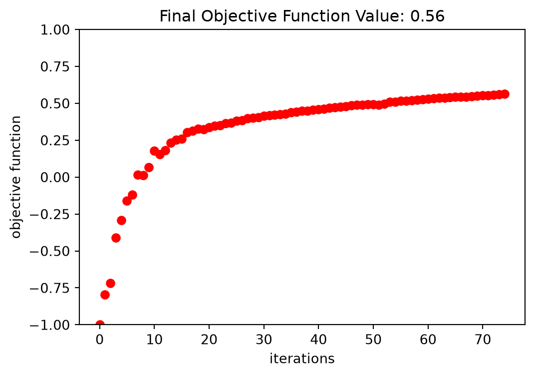
The final grating coupler structure is well binarized, with mostly black (eps_max) and white (eps_min) regions.
fig, ax = plt.subplots(1, figsize=(4, 4))
sim_final = make_adjoint_sim(final_par, beta=final_beta, unfold=True)
sim_final.plot_eps(z=0, source_alpha=0, monitor_alpha=0, ax=ax)
plt.show()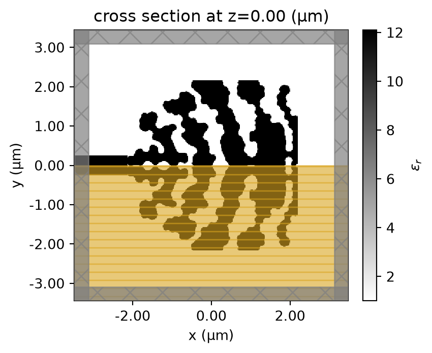
Once the inverse design is complete, we can visualize the field distributions and the wavelength dependent coupling efficiency.
# Field monitors to visualize the final fields.
field_xy = td.FieldMonitor(
    size=(td.inf, td.inf, 0),
    freqs=[freq],
    name="field_xy",
)

field_xz = td.FieldMonitor(
    size=(td.inf, 0, td.inf),
    freqs=[freq],
    name="field_xz",
)

# Monitor to compute the grating coupler efficiency.
gc_efficiency = td.ModeMonitor(
    center=[mon_pos_x, 0, 0],
    size=[0, mon_w, mon_h],
    freqs=freqs,
    mode_spec=mode_spec,
    name="gc_efficiency",
)

sim_final = sim_final.copy(update=dict(monitors=(field_xy, field_xz, gc_efficiency)))
sim_data_final = web.run(sim_final, task_name="inv_des_final")
09:31:39 UTC Created task 'inv_des_final' with resource_id 'fdve-bf94c3b7-933b-4f34-9460-e7cc235a164d' and task_type 'FDTD'.
             View task using web UI at
             'https://tidy3d.simulation.cloud/workbench?taskId=fdve-bf94c3b7-933
             b-4f34-9460-e7cc235a164d'.
Task folder: 'default'.
09:31:41 UTC Estimated FlexCredit cost: 0.212. This assumes the FDTD solver runs
             for the full simulation time; if early shutoff is reached, the
             billed cost can be lower. Use 'web.real_cost(task_id)' to get the
             billed FlexCredit cost after a simulation run.
09:31:42 UTC status = queued
             To cancel the simulation, use 'web.abort(task_id)' or
             'web.delete(task_id)' or abort/delete the task in the web UI.
             Terminating the Python script will not stop the job running on the
             cloud.
09:31:50 UTC status = preprocess
09:31:54 UTC starting up solver
running solver
09:32:06 UTC early shutoff detected at 12%, exiting.
status = postprocess
09:32:09 UTC status = success
09:32:11 UTC View simulation result at
             'https://tidy3d.simulation.cloud/workbench?taskId=fdve-bf94c3b7-933
             b-4f34-9460-e7cc235a164d'.
09:32:12 UTC Loading results from simulation_data.hdf5
mode_amps = sim_data_final["gc_efficiency"]
coeffs_f = mode_amps.amps.sel(direction="-")
power_0 = np.abs(coeffs_f.sel(mode_index=0)) ** 2
power_0_db = 10 * np.log10(power_0)

sim_plot = sim_final.updated_copy(symmetry=(0, 0, 0), monitors=(field_xy, field_xz, gc_efficiency))
sim_data_plot = sim_data_final.updated_copy(simulation=sim_plot)

f, ax = plt.subplots(2, 2, figsize=(8, 6), tight_layout=True)
sim_plot.plot_eps(z=0, source_alpha=0, monitor_alpha=0, ax=ax[0, 1])
ax[1, 0].plot(wl_range, power_0_db, "-k")
ax[1, 0].set_xlabel("Wavelength (um)")
ax[1, 0].set_ylabel("Power (db)")
ax[1, 0].set_ylim(-15, 0)
ax[1, 0].set_xlim(wl - bw / 2, wl + bw / 2)
ax[1, 0].set_title("Coupling Efficiency")
sim_data_plot.plot_field("field_xy", "E", "abs^2", z=0, ax=ax[1, 1])
ax[0, 0].plot(obj_vals, "ro")
ax[0, 0].set_xlabel("iterations")
ax[0, 0].set_ylabel("objective function")
ax[0, 0].set_ylim(-1, 1)
ax[0, 0].set_title(f"Final Objective Function Value: {obj_vals[-1]:.2f}")
plt.show()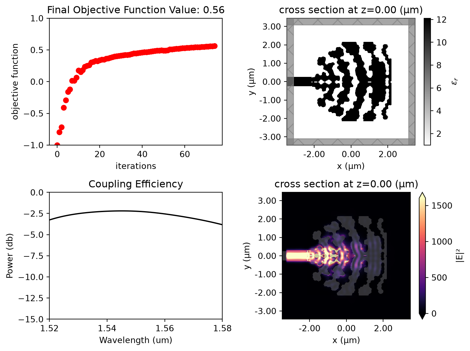
loss_db = max(power_0_db)
print(f"optimized loss of {loss_db:.2f} dB")
optimized loss of -2.20 dBExport to GDS
The Simulation object has the .to_gds_file convenience function to export the final design to a GDS file. In addition to a file name, it is necessary to set a cross-sectional plane (z = 0 in this case) on which to evaluate the geometry, a frequency to evaluate the permittivity, and a permittivity_threshold to define the shape boundaries in custom mediums. See the GDS export notebook for a detailed example on using .to_gds_file and other GDS related functions.
sim_final.to_gds_file(
    fname="./misc/inverse_designed_gc.gds",
    z=0,
    permittivity_threshold=(eps_max + eps_min) / 2,
    frequency=freq,
)


 TERMS & CONDITIONS


 How the process works:
 Try this real URL to see an example: