





import autograd.numpy as anp
import matplotlib.pyplot as plt
import numpy as np
import tidy3d as td
import tidy3d.web as web
from autograd.scipy.signal import convolve
from tidy3d.components.autograd import get_static
from tidy3d.plugins.autograd import adam, optimize

td.config.logging.level = "ERROR"  # disable warning about large number of source grid points
# Operating wavelength and frequency (units: µm)
wvl = 1.55
freq0 = td.C_0 / wvl

# Fiber geometry and refractive indices (approximate SMF-28 values)
d_smf_core = 8.2  # core diameter (µm)
n_smf_core = 1.449217  # core refractive index
n_smf_clad = 1.444  # cladding refractive index
n_design = 2.0  # refractive index of lens material (e.g., polymer or glass)
base_design_radius = 10  # radius of the lens base (µm)
fiber_length = 2  # length of fiber section in simulation (µm)

# Longitudinal layout (µm)
initial_height = 2.0  # starting height for all rings
free_space_length = 20.0  # propagation distance to focal plane
pml_buffer = wvl * 1.5  # buffer between structures and PML
monitor_buffer = 0.5  # buffer for source/monitor placement

# Simulation domain extent (µm)
sim_Ly = sim_Lz = 2 * base_design_radius + pml_buffer
sim_Lx = fiber_length + free_space_length
exit_monitor_size = 0.5  # size of the focal spot monitor

# Mesh parameterization
num_rings = 128  # number of concentric rings (design parameters)
ring_segments = 128  # polygon edges per ring (angular resolution)
smooth_sigma_frac = 0.02  # smoothing kernel width = num_rings * smooth_sigma_frac

# Height bounds for optimization (µm)
min_height, max_height = 0.1, 10.0
TIDY3D
LEARNING CENTER
Example Library

Point-symmetric fiber lens optimization
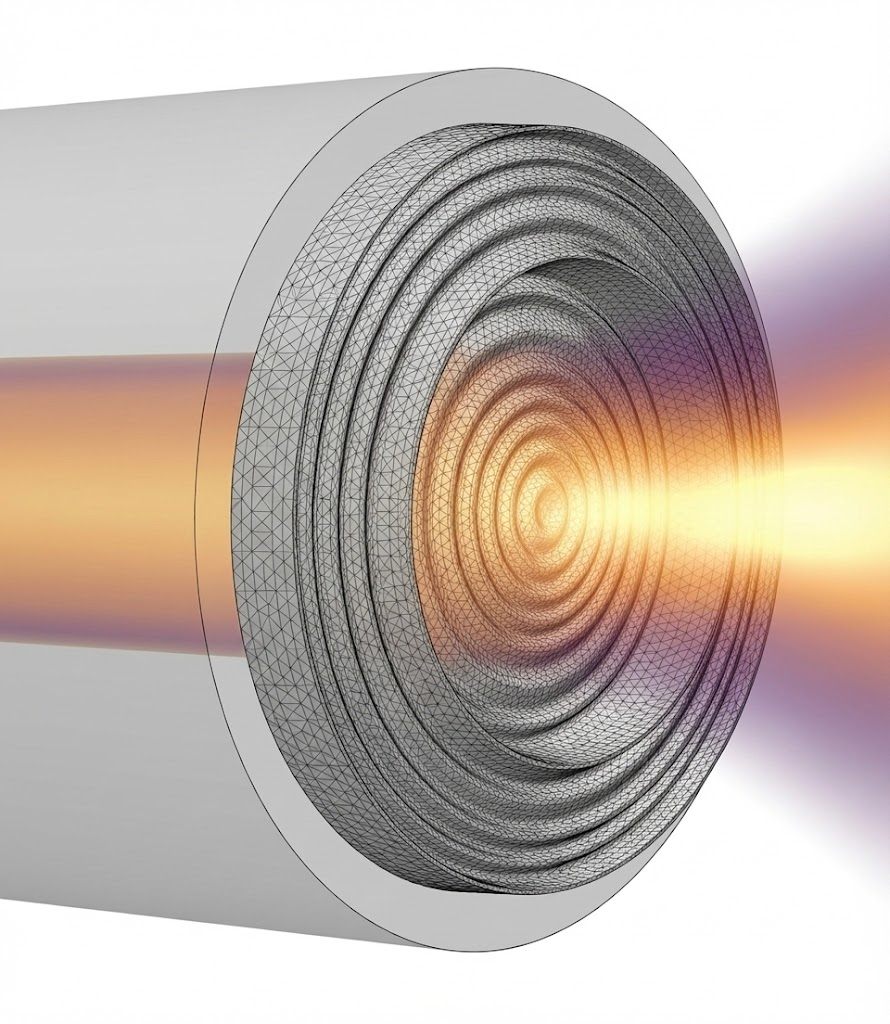
Fiber lenses, or microlenses fabricated directly on optical fiber tips, are essential components for beam shaping, focusing, and coupling in fiber-optic systems. Applications range from optical trapping and sensing to endoscopy and telecommunications.
In this notebook, we design a fiber lens by optimizing the 3D surface profile of a cylindrically symmetric structure attached to the tip of a single-mode fiber. The lens surface is parameterized as concentric rings whose heights are adjusted via gradient-based inverse design using Tidy3D’s native autograd support. The objective is to maximize the optical flux transmitted to a small focal region in front of the fiber.
We demonstrate free-form 3D shape optimization using a fully differentiable TriangleMesh geometry. Unlike topology optimization on a fixed pixel grid, this approach directly optimizes vertex positions of a surface mesh, enabling smooth, fabrication-ready freeform surfaces that can be exported directly to STL. This capability is particularly powerful for freeform optics where the optimal shape cannot be described by simple geometric primitives.
Initial Setup
We begin by importing the necessary packages and defining the key parameters for our simulation. The physical setup consists of:
- Fiber base: A single-mode fiber with core and cladding
- Lens structure: A cylinder-like design region whose top surface will be optimized
- Exit monitor: A small flux monitor at the target focal plane to measure focusing efficiency
The lens surface is discretized into num_rings concentric rings, each with an adjustable height. A Gaussian smoothing kernel is applied to ensure smooth, fabricable transitions between adjacent rings.
Simulation Setup
We now construct the base simulation containing the optical fiber without the lens structure. The fiber consists of a cylindrical core (higher refractive index) surrounded by cladding (lower refractive index). Both extend beyond the simulation boundaries to avoid edge effects at the PML.
INF = 1000
clad = td.Structure(
    geometry=td.Box.from_bounds((-INF, -INF, -INF), (fiber_length, INF, INF)),
    medium=td.Medium(permittivity=n_smf_clad**2),
)

core = td.Structure(
    geometry=td.Cylinder(
        center=clad.geometry.center,
        radius=d_smf_core / 2,
        length=clad.geometry.size[0],
        axis=0,
    ),
    medium=td.Medium(permittivity=n_smf_core**2),
)
We excite the fundamental mode of the fiber using a ModeSource. The mode solver automatically finds the guided mode, and we filter for TE polarization. The source emits a Gaussian pulse centered at the operating wavelength.
mode_source = td.ModeSource(
    size=(0, sim_Ly, sim_Lz),
    center=(monitor_buffer, 0, 0),
    source_time=td.GaussianPulse(freq0=freq0, fwidth=0.2 * freq0),
    mode_spec=td.ModeSpec(
        num_modes=1,
        target_neff=n_smf_core,
        sort_spec=td.ModeSortSpec(filter_key="TE_fraction", filter_reference=0.5),
        num_pml=(12, 12),
    ),
    direction="+",
    name="fiber_input",
)
A FluxMonitor is placed at the target focal plane to measure the transmitted optical power directly. The monitor size defines the “focal spot” region where we want to concentrate light.
exit_monitor = td.FluxMonitor(
    center=(sim_Lx - monitor_buffer, 0, 0),
    size=(0, exit_monitor_size, exit_monitor_size),
    freqs=[freq0],
    name="flux_exit",
    enable_adjoint=True,
)
We now assemble the base simulation with the fiber structures, source, and monitors. Optionally, a field monitor at z=0 can be added to visualize the field propagation along the optical axis.
def make_base_simulation(monitor_propagation=False):
    """Create the parameter-independent base simulation."""
    monitors = [exit_monitor]
    if monitor_propagation:
        monitors.append(
            td.FieldMonitor(
                center=(0, 0, 0), size=(td.inf, td.inf, 0), freqs=[freq0], name="field_z_0"
            )
        )

    propagation_distance = initial_height + free_space_length
    run_time = 10 * propagation_distance / td.C_0
    sim = td.Simulation(
        size=(sim_Lx, sim_Ly, sim_Lz),
        center=(sim_Lx / 2, 0, 0),
        grid_spec=td.GridSpec.auto(min_steps_per_wvl=20, wavelength=wvl),
        structures=[clad, core],
        sources=[mode_source],
        monitors=monitors,
        run_time=run_time,
    )

    return sim


base_sim = make_base_simulation()
Let’s visualize the base simulation in 2D cross-sections and 3D to verify the geometry and component placement.
f, (ax1, ax2) = plt.subplots(1, 2, tight_layout=True, figsize=(12, 4))
base_sim.plot(x=fiber_length / 2, ax=ax1)
ax1.set_title(f"Cross-section at x = {fiber_length / 2} µm")
base_sim.plot(z=0, ax=ax2)
ax2.set_title("Top view at z = 0")
plt.show()

base_sim.plot_3d()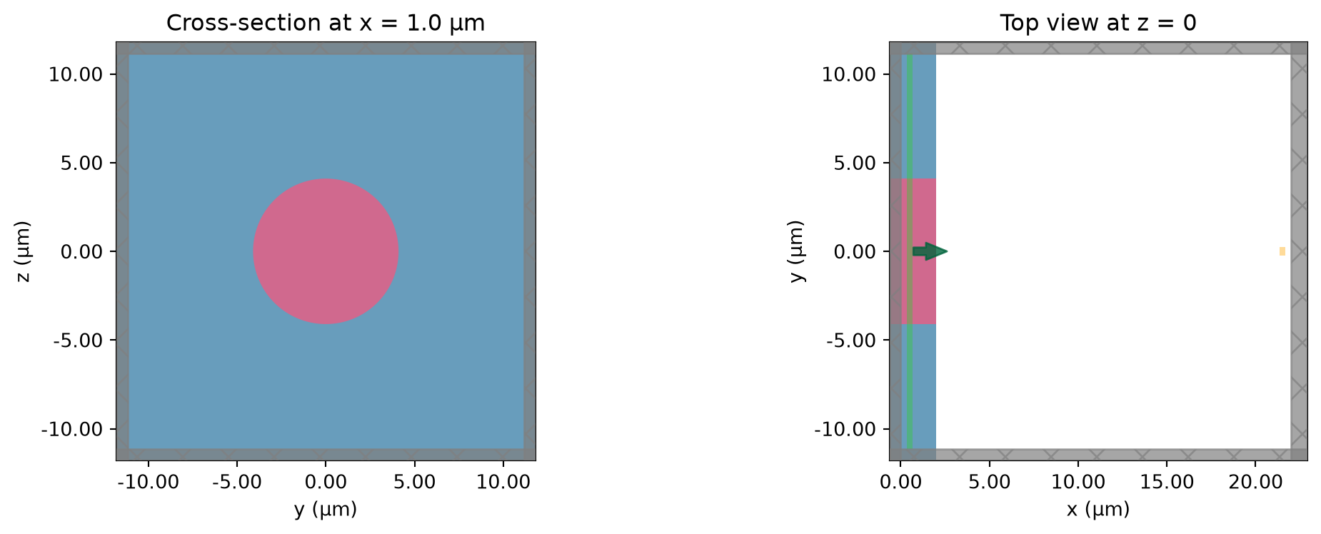
Mesh Construction
The lens geometry is defined as a TriangleMesh constructed from vertices and faces. The surface is parameterized as follows:
- Base ring: A circle at the fiber tip (height = 0) forming the lens base
- Concentric top rings: Each ring has an adjustable height controlled by the optimization parameters
- Center vertices: Top and bottom center points to close the mesh
The height profile is smoothed using a Gaussian kernel to ensure gradual transitions between adjacent rings, which improves manufacturability and avoids sharp discontinuities that could cause meshing issues.
def vertices_from_params(params):
    def smooth_param_profile(params):
        sigma = smooth_sigma_frac * len(params)
        if sigma == 0:
            return params
        pad = max(1, int(4 * sigma))

        # gaussian kernel
        x = anp.arange(-pad, pad + 1)
        k = anp.exp(-0.5 * (x / sigma) ** 2)
        k /= k.sum()

        # padding
        left_pad = params[1 : pad + 1][::-1]
        right_pad = params[-pad - 1 : -1][::-1]
        padded = anp.concatenate([left_pad, params, right_pad])

        # convolve
        smoothed = convolve(padded, k, mode="valid")
        return smoothed

    heights = smooth_param_profile(params)
    theta = anp.linspace(0.0, 2.0 * anp.pi, ring_segments, endpoint=False)
    cos_t = anp.cos(theta)
    sin_t = anp.sin(theta)

    rings = []

    # bottom base ring at height = 0
    X = anp.full(ring_segments, fiber_length)
    Y = base_design_radius * cos_t
    Z = base_design_radius * sin_t
    rings.append(anp.stack([X, Y, Z], axis=1))

    # rings for radius > 0
    ring_radii = np.linspace(0.0, base_design_radius, num_rings)
    for radius, h in zip(ring_radii[1:], heights[1:]):
        X = anp.full(ring_segments, fiber_length + h)
        Y = radius * cos_t
        Z = radius * sin_t
        rings.append(anp.stack([X, Y, Z], axis=1))

    vertices = anp.concatenate(rings, axis=0)

    # bottom and top center vertex
    top_center = anp.array([[fiber_length + heights[0], 0.0, 0.0]])
    bottom_center = anp.array([[fiber_length + 0.0, 0.0, 0.0]])

    vertices = anp.concatenate([vertices, top_center, bottom_center], axis=0)
    return vertices
Next, we define the triangular faces that connect the vertices. The vertex ordering must be counter-clockwise when viewed from outside the mesh to ensure correct surface normals.
def build_faces(num_rings):
    faces: list[list[int]] = []

    def ring_offset(i: int) -> int:
        return i * ring_segments

    K = num_rings - 1  # index of the outermost top ring

    top_center_idx = num_rings * ring_segments
    bottom_center_idx = top_center_idx + 1

    # ---- side wall between base ring and outermost top ring ----
    base = ring_offset(0)
    outer = ring_offset(K)
    for j in range(ring_segments):
        jn = (j + 1) % ring_segments
        faces.append([base + j, base + jn, outer + j])
        faces.append([base + jn, outer + jn, outer + j])

    # center fan on top surface: top_center ↔ ring 1
    inner_ring = ring_offset(1)
    for j in range(ring_segments):
        jn = (j + 1) % ring_segments
        faces.append([top_center_idx, inner_ring + j, inner_ring + jn])

    # ring-by-ring faces between top rings:
    # connect 1↔2, 2↔3, ..., (K-1)↔K
    for i in range(1, K):
        r0 = ring_offset(i)
        r1 = ring_offset(i + 1)
        for j in range(ring_segments):
            jn = (j + 1) % ring_segments
            faces.append([r0 + j, r1 + j, r0 + jn])
            faces.append([r0 + jn, r1 + j, r1 + jn])

    # ---- bottom disk: fan from bottom_center to base ring ----
    base_start = ring_offset(0)
    for j in range(ring_segments):
        jn = (j + 1) % ring_segments
        faces.append([bottom_center_idx, base_start + jn, base_start + j])
    faces = anp.array(faces, dtype=int)
    return faces
We can now construct the complete mesh from a parameter vector. The mesh_from_params function computes vertices from the parameters and combines them with the precomputed face connectivity to create a TriangleMesh object.
FACE_ARRAY = build_faces(num_rings)


def mesh_from_params(params):
    vertices = vertices_from_params(params)
    triangles = vertices[FACE_ARRAY]
    mesh = td.TriangleMesh.from_triangles(triangles)
    return mesh
Mesh Visualization
Before optimization, let’s verify the mesh construction by creating a lens with randomized ring heights. This helps confirm that the geometry, smoothing, and triangulation work correctly.
def get_fiber_design_sim(params, monitor_propagation=False):
    """Create simulation with fiber and parameterized lens structure."""
    mesh = mesh_from_params(params)
    base_sim = make_base_simulation(monitor_propagation=monitor_propagation)
    medium = td.Medium(permittivity=n_design**2)
    design_structure = td.Structure(geometry=mesh, medium=medium, name="lens")
    new_structures = [*base_sim.structures, design_structure]
    return base_sim.updated_copy(structures=new_structures, validate=True)


# Create example with random perturbations
example_params = np.full(num_rings, initial_height) + np.random.randn(num_rings) * 0.5
example_design_sim = get_fiber_design_sim(example_params)
example_design_sim.plot_3d()  # 3D plot
example_design_sim.plot(z=0)  # 2D plot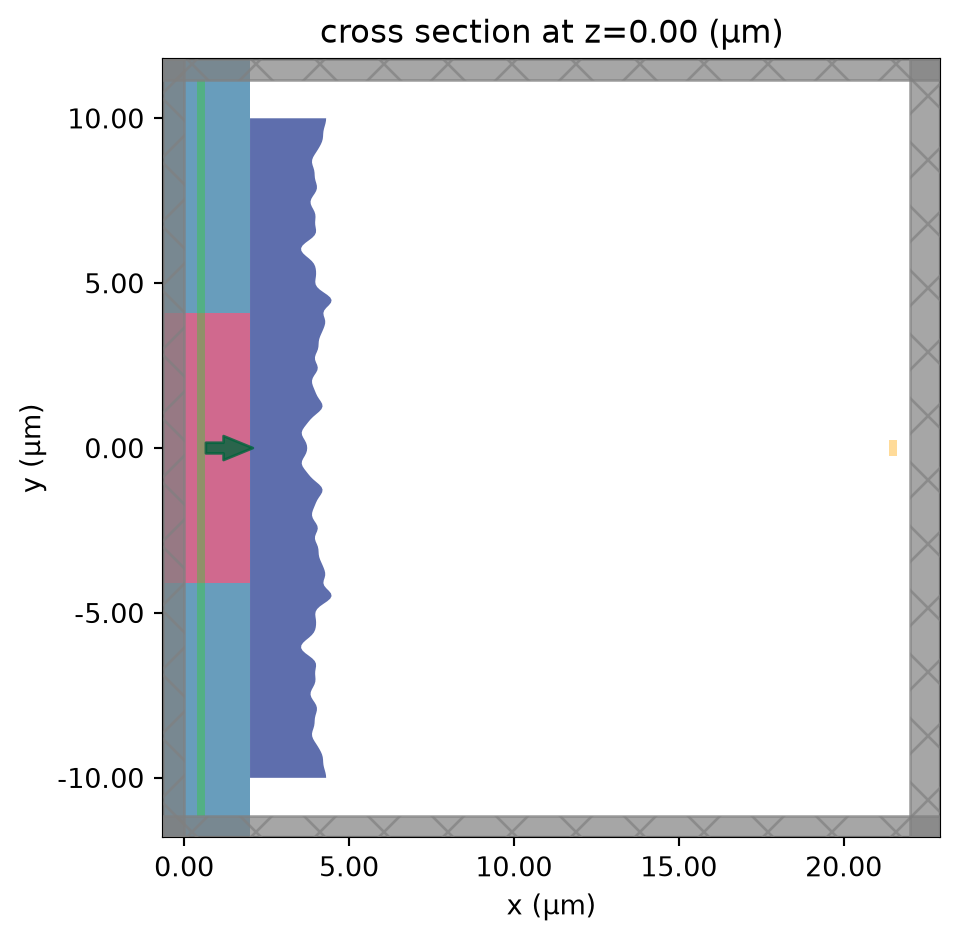
Objective Function
The objective function defines what we want to optimize. Here, we maximize the optical power (flux) transmitted through the exit monitor at the focal plane. The function:
- Constructs a simulation from the current parameters
- Runs the FDTD simulation via
web.run() - Extracts and returns the flux from the flux monitor
def objective(params):
    """Compute the flux at the focal plane for a given set of ring heights."""
    sim = get_fiber_design_sim(params)
    sim_data = web.run(sim, task_name="fiber_lens_opt", verbose=False)
    flux = sim_data["flux_exit"].flux.data
    return flux
Optimization
We use Tidy3D’s Adam optimizer to iteratively improve the lens design. The optimize does the actual iterative optimization. It requires the starting parameters (params0), the optimizer instance, the number of steps to run, optionally parameter bounds, a callback which is run on every iteration, and the optimization direction.
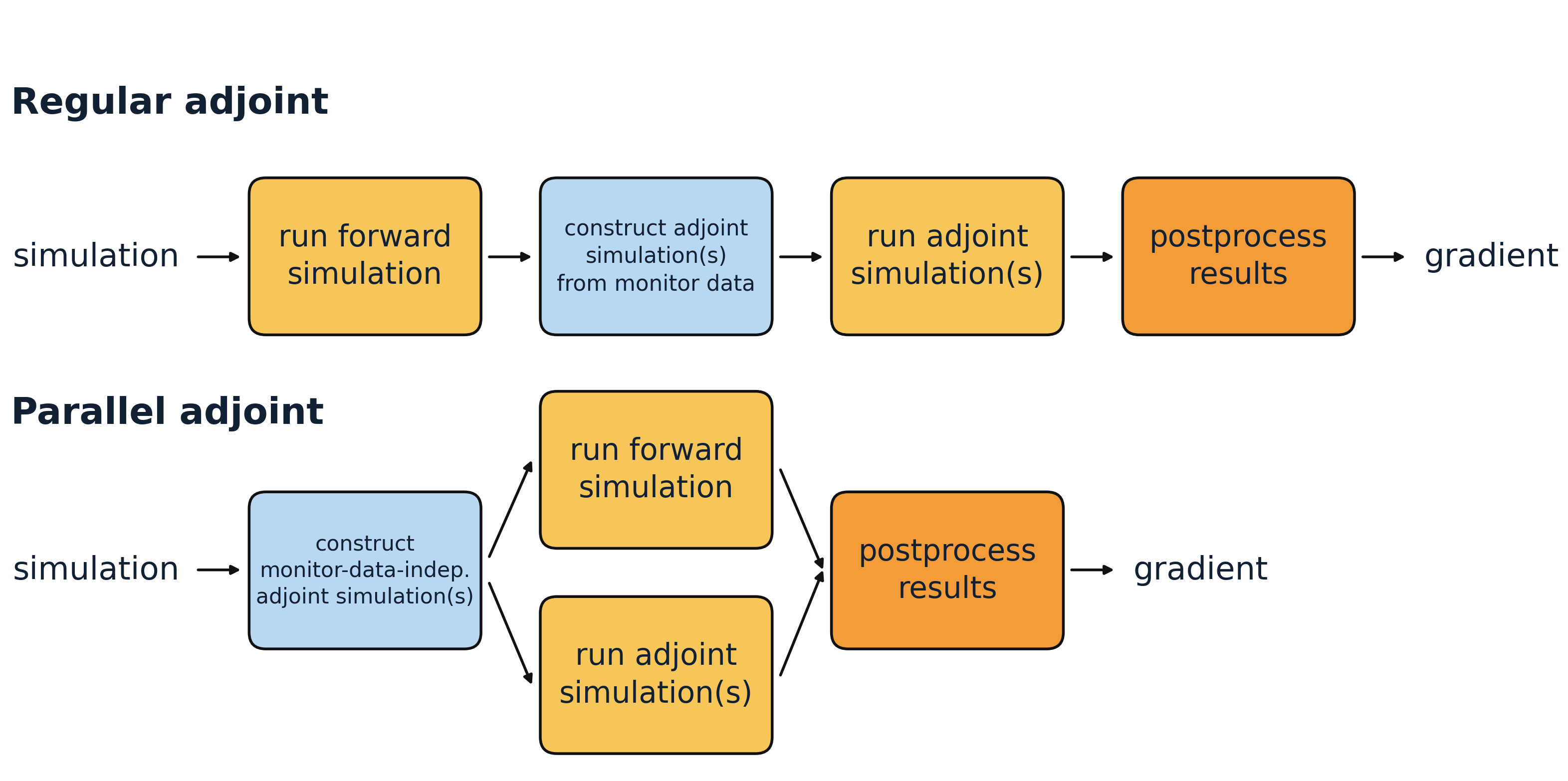
The gradient is computed efficiently via the adjoint method: only two simulations (forward + adjoint) are needed per step, regardless of the 128 design parameters.
# Optimization configuration
num_steps = 25
learning_rate = 0.1

# Initialize parameters (uniform height) and optimizer
params0 = anp.full(num_rings, initial_height, dtype=float)
optimizer = adam(learning_rate=learning_rate)


def report_step(current_params, grad, state, step_index, objective_val):
    grad_norm = float(np.linalg.norm(grad))
    print(
        f"Step {step_index + 1:02d}/{num_steps}: flux = {float(objective_val):.4e}, ||∇|| = {grad_norm:.4e}"
    )


params, opt_state, history = optimize(
    objective,
    params0=params0,
    optimizer=optimizer,
    num_steps=num_steps,
    bounds=(min_height, max_height),
    callback=report_step,
    direction="max",
)
Step 01/25: flux = 5.6067e-03, ||∇|| = 8.6056e-03
Step 02/25: flux = 1.3564e-02, ||∇|| = 9.5117e-03
Step 03/25: flux = 1.9683e-02, ||∇|| = 7.9498e-03
Step 04/25: flux = 2.4573e-02, ||∇|| = 8.1977e-03
Step 05/25: flux = 2.7097e-02, ||∇|| = 1.0408e-02
Step 06/25: flux = 2.8608e-02, ||∇|| = 1.0657e-02
Step 07/25: flux = 3.0063e-02, ||∇|| = 9.9798e-03
Step 08/25: flux = 3.1285e-02, ||∇|| = 9.2707e-03
Step 09/25: flux = 3.1822e-02, ||∇|| = 9.7427e-03
Step 10/25: flux = 3.2152e-02, ||∇|| = 1.0404e-02
Step 11/25: flux = 3.2829e-02, ||∇|| = 9.2300e-03
Step 12/25: flux = 3.3369e-02, ||∇|| = 7.6085e-03
Step 13/25: flux = 3.3805e-02, ||∇|| = 8.2213e-03
Step 14/25: flux = 3.4679e-02, ||∇|| = 7.4624e-03
Step 15/25: flux = 3.5596e-02, ||∇|| = 6.1975e-03
Step 16/25: flux = 3.6124e-02, ||∇|| = 5.7143e-03
Step 17/25: flux = 3.6528e-02, ||∇|| = 5.0211e-03
Step 18/25: flux = 3.6698e-02, ||∇|| = 4.8604e-03
Step 19/25: flux = 3.6805e-02, ||∇|| = 5.5941e-03
Step 20/25: flux = 3.7151e-02, ||∇|| = 6.1068e-03
Step 21/25: flux = 3.7636e-02, ||∇|| = 5.4431e-03
Step 22/25: flux = 3.8224e-02, ||∇|| = 4.8717e-03
Step 23/25: flux = 3.8597e-02, ||∇|| = 5.1774e-03
Step 24/25: flux = 3.9002e-02, ||∇|| = 5.1325e-03
Step 25/25: flux = 3.9491e-02, ||∇|| = 4.0352e-03Results Analysis
Let’s analyze the optimization results by plotting the convergence history and visualizing the optimized lens alongside the field distribution. The optimized design typically exhibits a wave-like (Fresnel-like) surface profile that focuses light to the target region.
def plot_history(history):
    """Plot the optimization convergence history."""
    plt.figure(figsize=(8, 4))
    plt.plot(np.arange(1, len(history) + 1), history, "o-", linewidth=2, markersize=4)
    plt.xlabel("Optimization Step")
    plt.ylabel("Flux at Focal Plane")
    plt.title("Optimization Convergence")
    plt.grid(True, alpha=0.3)
    plt.tight_layout()
    plt.show()


def plot_design_and_field(sim, data):
    """Plot the lens geometry and field distribution side by side."""
    f, (ax1, ax2) = plt.subplots(1, 2, tight_layout=True, figsize=(12, 4))
    sim.plot(z=0, ax=ax1)
    ax1.set_title("Optimized Lens (top view)")
    data.plot_field("field_z_0", "E", "abs^2", ax=ax2)
    ax2.set_title("Field Intensity |E|²")
    plt.show()


# Plot convergence
plot_history(history["objective_fn_val"])

# Run final simulation with propagation monitor
final_sim = get_fiber_design_sim(params, monitor_propagation=True)
final_data = web.run(
    final_sim, task_name="fiber_lens_final", verbose=False, path="fiber_lens_final.hdf5"
)

# Report final performance
final_flux = final_data["flux_exit"].flux.values
print(f"\nFinal flux at focal plane: {final_flux.item():.4e}")

# Visualize results
plot_design_and_field(final_sim, final_data)
final_sim.plot_3d()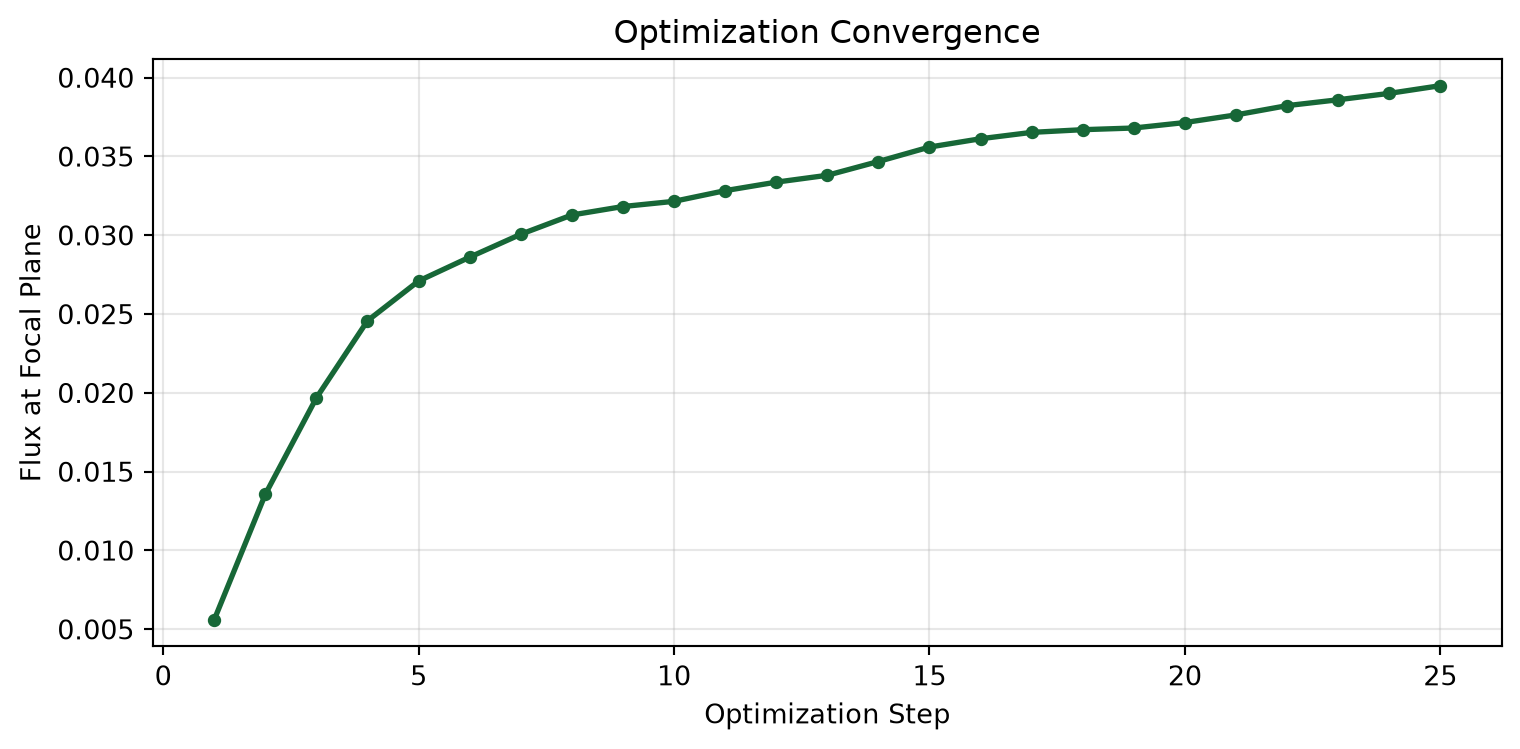
Final flux at focal plane: 3.9822e-02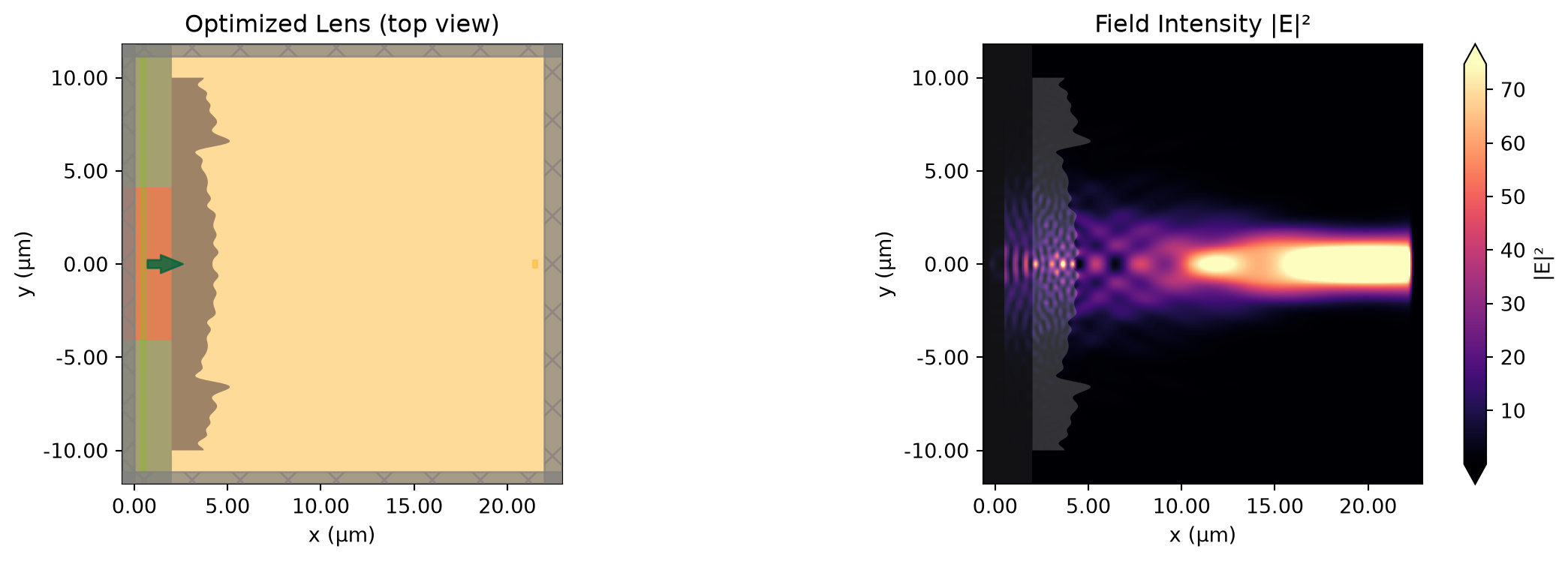
Export Results
Finally, we save the optimized parameters and export the lens geometry as an STL file for fabrication or further analysis in CAD software.
# Save optimized parameters
npy_export_path = "misc/fiber_lens_params.npy"
np.save(npy_export_path, get_static(params))
print(f"Saved {num_rings} optimized ring heights to '{npy_export_path}'")

# Export mesh as STL
mesh = mesh_from_params(params)
stl_export_path = "misc/fiber_lens.stl"
mesh.to_stl(stl_export_path)
print(f"Exported lens geometry to '{stl_export_path}'")
Saved 128 optimized ring heights to 'misc/fiber_lens_params.npy'
Exported lens geometry to 'misc/fiber_lens.stl'Summary
In this notebook, we demonstrated inverse design of a fiber lens using Tidy3D’s native autograd support. Key takeaways:
- TriangleMesh parameterization: Complex 3D surfaces can be optimized by making vertex positions differentiable
- Gaussian smoothing: Applying a smoothing kernel to parameters ensures manufacturable designs
- Adjoint efficiency: Gradients for 128 parameters are computed with just 2 simulations per step
- STL export: Optimized geometries can be directly exported for fabrication
Related Examples
- Inverse Design Overview: Introduction to autograd in Tidy3D
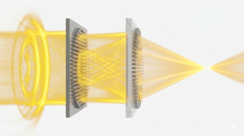
- Metalens Optimization: Optimizing a flat metalens for focusing
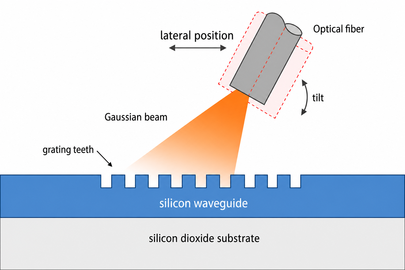
- Grating Coupler: Inverse design of fiber-to-chip coupling
- Boundary Gradients: Shape optimization fundamentals


 TERMS & CONDITIONS


 How the process works:
 Try this real URL to see an example: