





import matplotlib.pyplot as plt
import numpy as np
import tidy3d as td
import trimesh
TIDY3D
LEARNING CENTER
Tidy3D Python

Complete this course to
earn 50 FlexCredits
Credits are added to your account when all course items are checked in green.
Defining complex geometries using trimesh
Tidy3D offers four primitive geometric shapes: Box, Cylinder, Sphere, and PolySlab. An extensive array of intricate geometrical configurations can be defined from these fundamental building blocks by manipulating their properties and hierarchical arrangements. For instance, our tutorials on the Luneburg lens waveguide size converter and the Fresnel lens showcase the creation of curved surfaces through the strategic layering of cylindrical elements.
Beyond the in-built primitives, Tidy3D accommodates external geometrical specifications in either the gds or stl file formats, allowing users to import custom geometries created in their preferred design tools. Additionally, compatibility with external libraries like gdstk and shapely opens the gateway to even more complex geometric possibilities. Using gdstk to create various waveguide structures has been demonstrated in various examples such as the polarization splitter and rotator based on 90 degree bends.
In this tutorial, we’ll introduce an alternative avenue for crafting complex geometries using the trimesh library. Through examples featuring a torus, an ellipsoid, and a custom planar solid with holes, we’ll guide you through the process of defining a mesh structure that is directly usable in Tidy3D simulations.
Remember to install Tidy3D as pip install "tidy3d[trimesh]", which will install optional dependencies needed for processing surface meshes.
Built-in Geometries
First off all, trimesh provides some built-in geometries such as ring (annulus), box, capsule, cone, cylinder, and so on. Let’s create a ring as an example.
After the mesh is created, we can visualize the mesh in 3D.
n_sections = 100 # how many sections to discretize the mesh
# create a ring mesh
ring_mesh = trimesh.creation.annulus(r_min=9, r_max=10, height=1, sections=n_sections)
# plot the mesh
ring_mesh.show()To use this geometry in a Tidy3D simulation, we need to convert the mesh into a Tidy3D TriangleMesh geometry. The from_trimesh() method conveniently converts a mesh to a Tidy3D geometry. From there, you can further define Tidy3D Structure and put it into a Simulation.
# define a tidy3d geometry from a mesh
ring_geo = td.TriangleMesh.from_trimesh(ring_mesh)
# plot a 2d cross section of the geometry
ring_geo.plot(z=0)
plt.show()13:59:26 UTC WARNING: Plotting a 'TriangleMesh' may give inconsistent results if the mesh is not unionized. We recommend unionizing all meshes before import. A 'PermittivityMonitor' can be used to check that the mesh is loaded correctly.
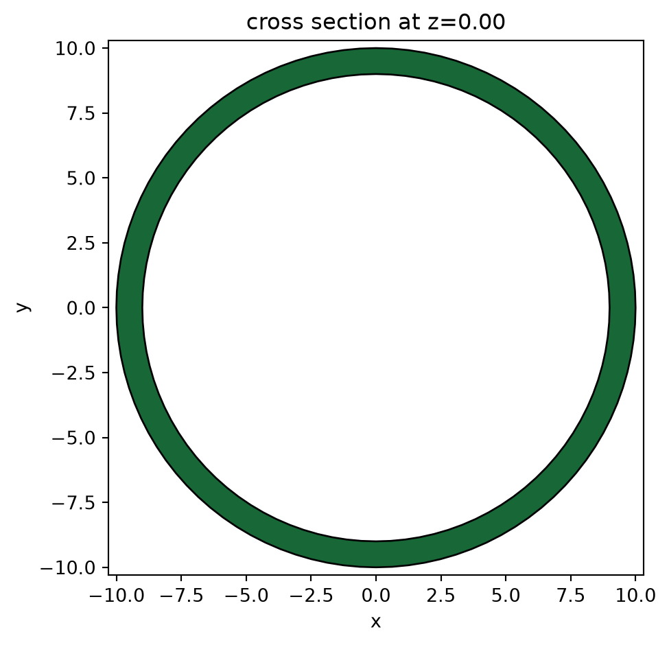
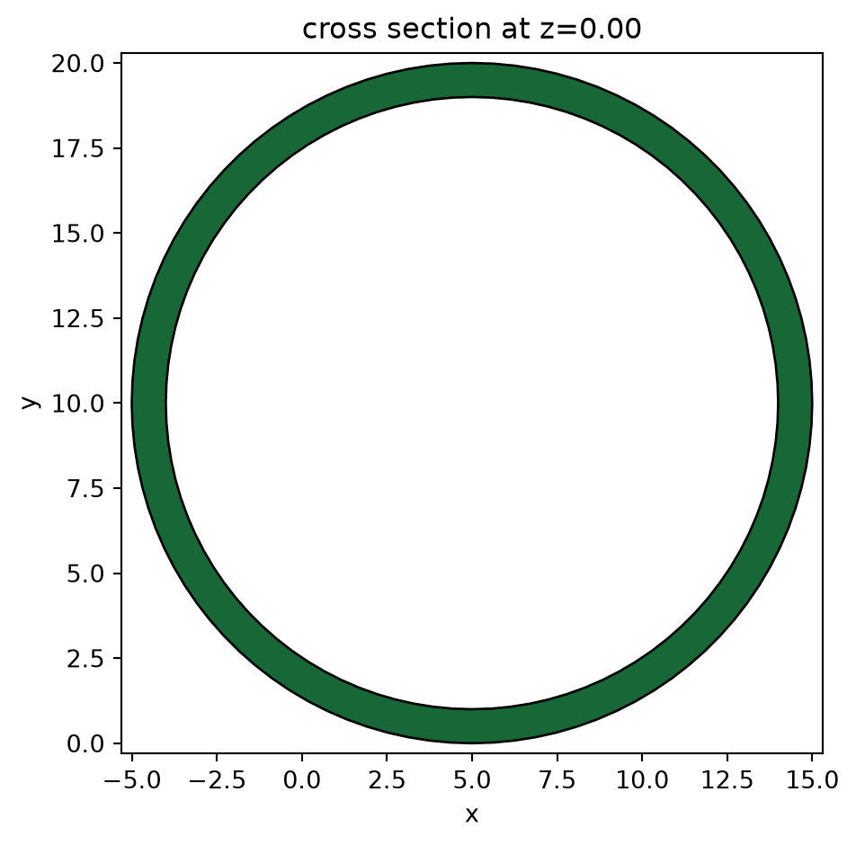
In addition, you can easily apply operations to a mesh such as translation and rotation. Here we demonstrate how to translate the previously created ring by a vector (5, 10, 0). The resulting ring is centered at (5, 10, 0).
# translate the ring
ring_mesh.apply_translation([5, 10, 0])
# define a tidy3d geometry from a mesh
ring_geo = td.TriangleMesh.from_trimesh(ring_mesh)
ring_geo.plot(z=0)
plt.show()WARNING: Plotting a 'TriangleMesh' may give inconsistent results if the mesh is not unionized. We recommend unionizing all meshes before import. A 'PermittivityMonitor' can be used to check that the mesh is loaded correctly.
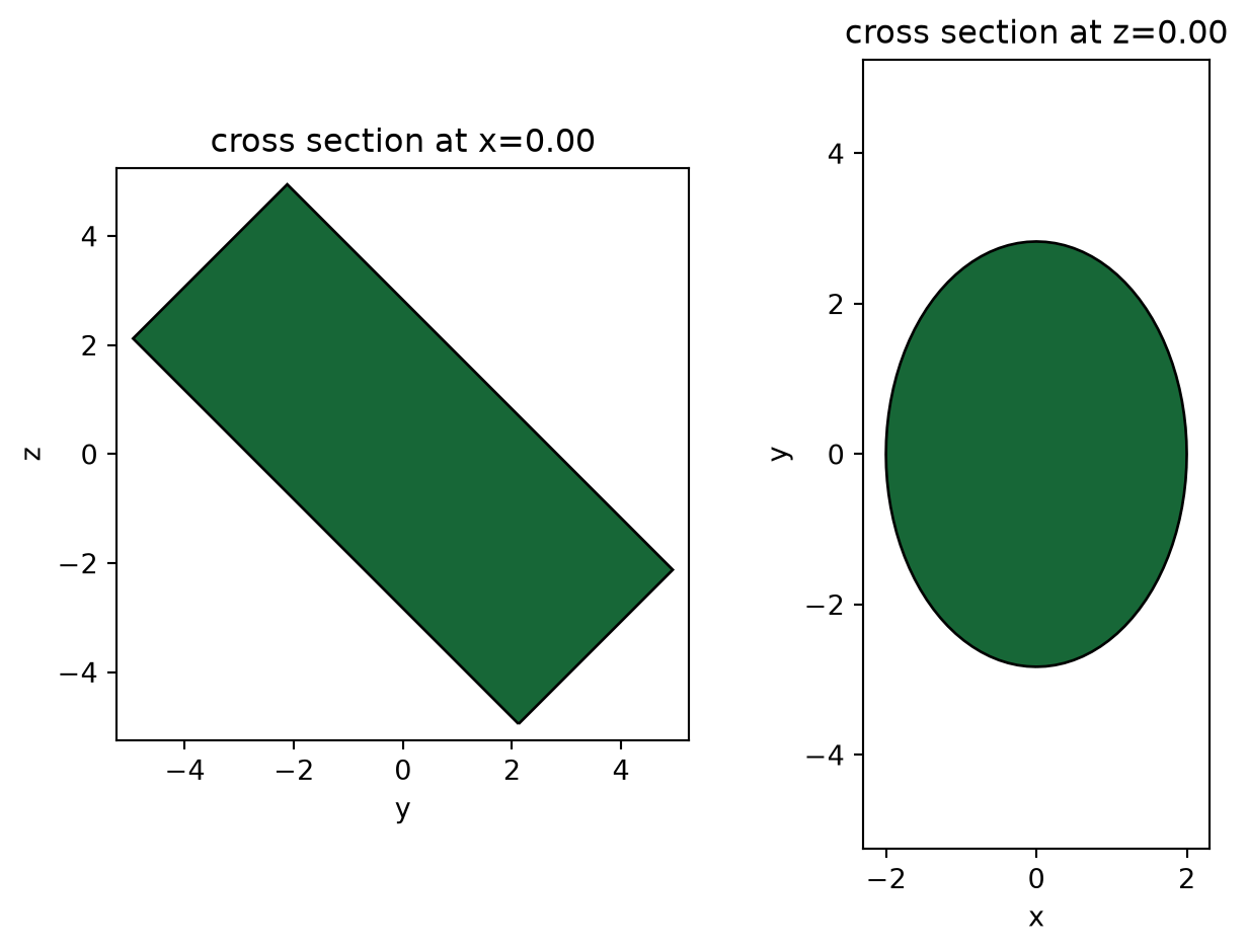
In a grating coupler simulation, very often we want to use a tilted cylinder to model the fiber core at an angle. This can be done with the help of trimesh too. First create a cylinder and then apply a rotation transformation to it.
# create a cylinder
cylinder_mesh = trimesh.creation.cylinder(radius=2, height=10, sections=n_sections)
# apply rotation
rot_x = trimesh.transformations.rotation_matrix(np.radians(45), [1, 0, 0])
cylinder_mesh.apply_transform(rot_x)
cylinder_mesh.show()Convert the mesh into a Tidy3D geometry and plot the cross section views.
cylinder_geo = td.TriangleMesh.from_trimesh(cylinder_mesh)
fig, (ax1, ax2) = plt.subplots(1, 2, tight_layout=True)
cylinder_geo.plot(x=0, ax=ax1)
cylinder_geo.plot(z=0, ax=ax2)
plt.show()WARNING: Plotting a 'TriangleMesh' may give inconsistent results if the mesh is not unionized. We recommend unionizing all meshes before import. A 'PermittivityMonitor' can be used to check that the mesh is loaded correctly.
WARNING: Plotting a 'TriangleMesh' may give inconsistent results if the mesh is not unionized. We recommend unionizing all meshes before import. A 'PermittivityMonitor' can be used to check that the mesh is loaded correctly.
Defining Complex Geometries from Vertices and Faces
Defining a Box
Beyond the built-in geometries, much more complex geometries can be created in trimesh. To do so, we need to define the vertices and triangular faces for the geometry.
First we demonstrate the idea by defining a simple box. The eight vertices of the box can be easily calculated given the width, height, and depth of the box. Then, a triangular face can be defined from three vertex indices. The box has six rectangular faces, which can be broken down into twelve triangular faces. Note that when defining the faces, we need to be careful about the order of the vertex indices to make sure the surface normal direction is consistent.
def create_box(width, height, depth):
# create vertices
vertices = np.array(
[
[+width / 2, +height / 2, +depth / 2], # front top right
[-width / 2, +height / 2, +depth / 2], # front top left
[-width / 2, -height / 2, +depth / 2], # front bottom left
[+width / 2, -height / 2, +depth / 2], # front bottom right
[+width / 2, +height / 2, -depth / 2], # back top right
[-width / 2, +height / 2, -depth / 2], # back top left
[-width / 2, -height / 2, -depth / 2], # back bottom left
[+width / 2, -height / 2, -depth / 2], # back bottom right
]
)
# define faces
faces = np.array(
[
[0, 1, 2], # front face
[0, 2, 3],
[4, 6, 5], # back face
[4, 7, 6],
[0, 4, 5], # left face
[0, 5, 1],
[3, 2, 6], # right face
[3, 6, 7],
[1, 5, 6], # top face
[1, 6, 2],
[0, 3, 7], # bottom face
[0, 7, 4],
]
)
return trimesh.Trimesh(vertices=vertices, faces=faces, process=False)Create a box using the above function to verify that it works as expected.
box_mesh = create_box(1, 2, 3)
box_mesh.show()Defining a Torus
The previous box example is just to illustrate the idea of defining a mesh from vertices and faces. Next we showcase how to define a torus and a ellipsoid using the same approach. Both geometries are difficult to define natively in Tidy3D.
Let’s start with the torus. The vertices of the torus are given by
\[ x = (R+r\cos\phi)\cos\theta \]
\[ y =( R+r\cos\phi)\sin\theta \]
\[ z =r\sin\phi, \]
where \(R\) is the radius of the major circle, \(r\) is the radius of the minor circle, \(\phi\) is the angle that parameterizes the minor circle and \(\theta\) is the angle that parameterizes the major circle. major_segments and minor_segments control the number of segments in the major and minor circles, respectively.
def create_torus(major_radius, minor_radius, major_segments, minor_segments):
# initialize empty lists to store the torus vertices and faces
vertices = []
faces = []
# create vertices
# loop over the major circle (the "doughnut" shape)
for i in range(major_segments):
# calculate the angle for the current major segment
theta = i * 2 * np.pi / major_segments
# loop over the minor circle (the "cross-section" of the doughnut)
for j in range(minor_segments):
# calculate the angle for the current minor segment
phi = j * 2 * np.pi / minor_segments
# calculate the x, y, z coordinates for the current vertex
# the vertex lies on the smaller circle, which is then rotated around the origin
x = (major_radius + minor_radius * np.cos(phi)) * np.cos(theta)
y = (major_radius + minor_radius * np.cos(phi)) * np.sin(theta)
z = minor_radius * np.sin(phi)
# append the current vertex to the vertices list
vertices.append([x, y, z])
# create faces
# loop over the major circle again to create faces
for i in range(major_segments):
# loop over the minor circle to create faces
for j in range(minor_segments):
# calculate indices for the next major and minor segments
# use modulo to wrap-around at the end
next_i = (i + 1) % major_segments
next_j = (j + 1) % minor_segments
# indices of vertices around the face, based on the current and next segments
v1 = i * minor_segments + j
v2 = next_i * minor_segments + j
v3 = next_i * minor_segments + next_j
v4 = i * minor_segments + next_j
# create two triangular faces to form a quad face connecting these vertices
# this covers the current segment of the torus
faces.append([v1, v2, v4])
faces.append([v2, v3, v4])
# create mesh using the generated vertices and faces
return trimesh.Trimesh(vertices=vertices, faces=faces)Create a specific torus and plot it.
torus_mesh = create_torus(
major_radius=2,
minor_radius=0.3,
major_segments=n_sections,
minor_segments=n_sections,
)
torus_mesh.show()Defining an Ellipsoid
As the last example, we showcase how to define an ellipsoid. The vertices of an ellipsoid are given by
\[ x = a\sin\theta \cos\phi \]
\[ y=b\sin\theta \sin\phi \]
\[ z=c\cos\theta, \]
where \(a\), \(b\), and \(c\) are radii along the \(x\), \(y\), and \(z\) axes, respectively. u_segments and v_segments control the number of segments in the latitude and longitude, respectively.
def create_ellipsoid(a, b, c, u_segments, v_segments):
# initialize empty lists for vertices and faces
vertices = []
faces = []
# create vertices
for i in range(u_segments + 1):
theta = i * np.pi / u_segments # angle for the latitude (0 to pi)
for j in range(v_segments + 1):
phi = j * 2 * np.pi / v_segments # angle for the longitude (0 to 2*pi)
# compute vertex position using ellipsoidal equations
x = a * np.sin(theta) * np.cos(phi)
y = b * np.sin(theta) * np.sin(phi)
z = c * np.cos(theta)
vertices.append([x, y, z])
# create faces
for i in range(u_segments):
for j in range(v_segments):
# compute indices for vertices
v1 = i * (v_segments + 1) + j
v2 = (i + 1) * (v_segments + 1) + j
v3 = (i + 1) * (v_segments + 1) + (j + 1)
v4 = i * (v_segments + 1) + (j + 1)
# create faces using the vertices
faces.append([v1, v2, v3])
faces.append([v1, v3, v4])
# create mesh using the generated vertices and faces
return trimesh.Trimesh(vertices=vertices, faces=faces)Create a specific ellipsoid and plot it.
ellipsoid_mesh = create_ellipsoid(a=1.3, b=0.4, c=0.3, u_segments=100, v_segments=100)
ellipsoid_mesh.update_faces(ellipsoid_mesh.nondegenerate_faces())
ellipsoid_mesh.show()Lastly, we demonstrate again how to define Tidy3D Structures from the mesh. We will put the previously defined torus and ellipsoid into a Simulation and plot the cross section of it. As expected, we see a ring and an ellipse in the plot.
# define tidy3d geometries from the torus mesh and ellipsoid mesh
torus_geo = td.TriangleMesh.from_trimesh(torus_mesh)
ellipsoid_geo = td.TriangleMesh.from_trimesh(ellipsoid_mesh)
# define tidy3d structures from the geometries
torus_structure = td.Structure(geometry=torus_geo, medium=td.Medium(permittivity=2))
ellipsoid_structure = td.Structure(
geometry=ellipsoid_geo, medium=td.Medium(permittivity=2)
)
# put the structures into a simulation
sim = td.Simulation(
size=(5, 5, 5),
structures=[torus_structure, ellipsoid_structure],
grid_spec=td.GridSpec.auto(min_steps_per_wvl=25, wavelength=1),
run_time=1e-12,
)
# plot the cross section of the simulation
sim.plot(z=0)
plt.show()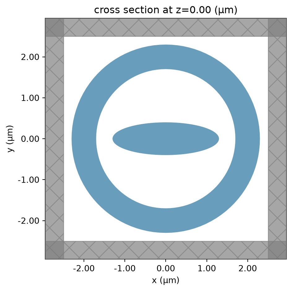
Revolving a Polygon Profile
Another powerful way to generate complex surfaces is to revolve a 2D polygon around an axis. This is especially handy for axisymmetric components such as lenses, resonators, or tapered fibers where the cross section is easier to sketch in 2D. We can sketch the profile as a list of vertices and let trimesh sweep it through 360° to obtain a solid mesh.
def revolve_polygon(
vertices,
segments=128,
rotation_angle_deg=0,
rotation_axis=np.array([1, 0, 0]),
):
"""Return a revolved `trimesh.Trimesh` by sweeping a 2D polygon about the z-axis.
Parameters
----------
vertices : (N, 2) np.ndarray
Polygon vertices ordered along the profile in the x-z plane.
segments : int, optional
Number of azimuthal segments used in the revolution; higher values give smoother meshes.
rotation_angle_deg : float, optional
Additional rotation applied to the mesh (in degrees) about `rotation_axis` after revolution.
rotation_axis : array-like, optional
Axis for the optional post-rotation, expressed in Cartesian coordinates.
"""
rotation_angle = np.deg2rad(rotation_angle_deg)
mesh = trimesh.creation.revolve(
vertices,
segments=segments,
angle=2 * np.pi,
)
if rotation_angle != 0:
rotation_matrix = trimesh.transformations.rotation_matrix(
rotation_angle,
rotation_axis,
point=None,
)
mesh.apply_transform(rotation_matrix)
return mesh# define a simple aspheric-like lens profile in the x-z plane
lens_vertices = np.array(
[
[0.0, 0.0],
[0.5, 0.0],
[0.8, 0.15],
[0.9, 0.35],
[0.5, 0.6],
[0.0, 0.6],
]
)
# visualize the 2D polygon profile before revolving
fig, ax = plt.subplots(tight_layout=True)
closed_vertices = np.vstack([lens_vertices, lens_vertices[0]])
ax.plot(closed_vertices[:, 0], closed_vertices[:, 1], marker="o")
ax.fill(closed_vertices[:, 0], closed_vertices[:, 1], alpha=0.2)
ax.set_aspect("equal")
ax.set_xlabel("x (μm)")
ax.set_ylabel("z (μm)")
ax.set_title("Polygon profile prior to revolution")
plt.show()
lens_mesh = revolve_polygon(lens_vertices, segments=180)
lens_mesh.show()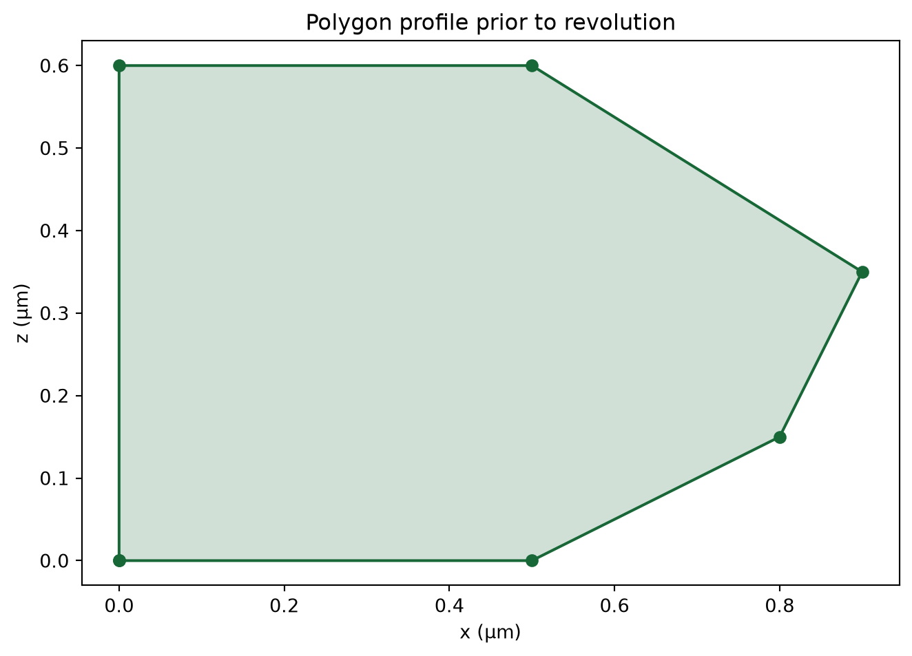
Defining a PlanarSolid Object
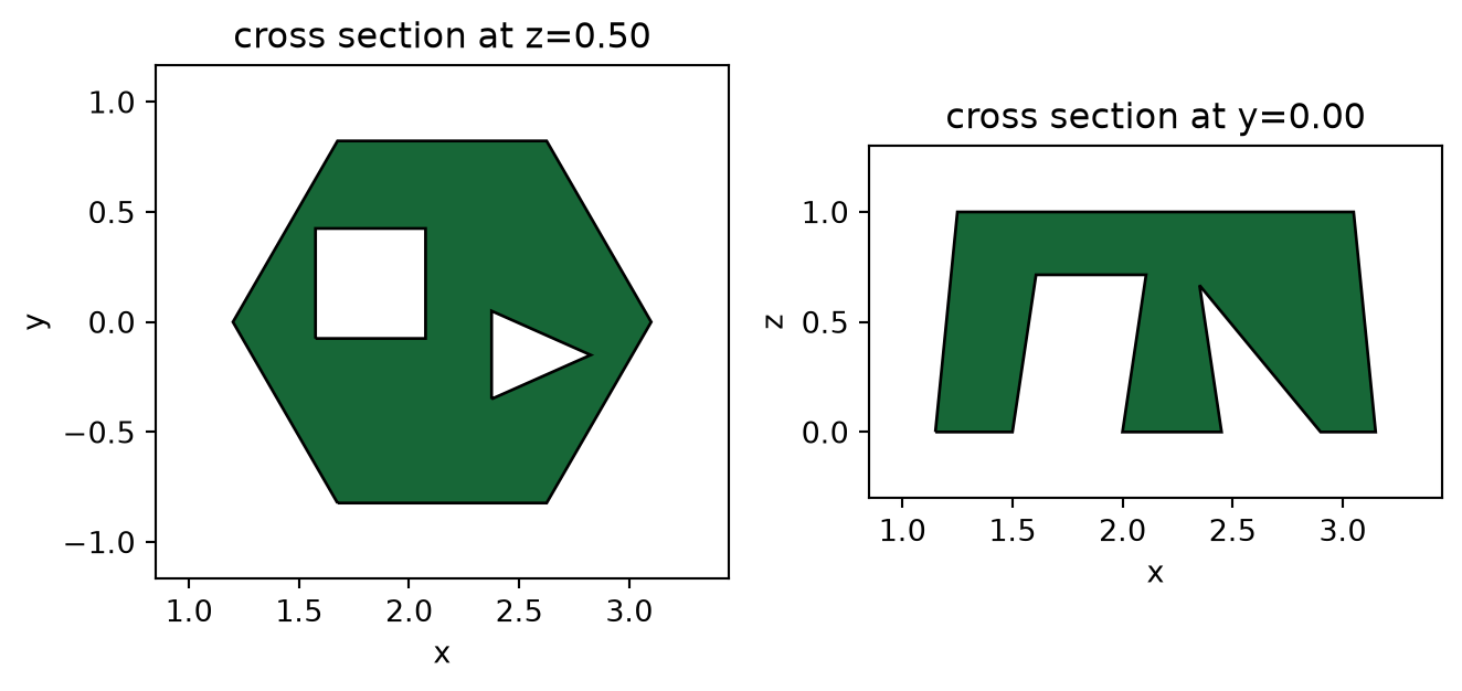
For shapes that are neither primitives nor revolved profiles, trimesh can build a planar solid: a set of vertices connected by flat facets, each optionally punctured by holes. Because every facet is defined independently, this is also handy when a fabricated sidewall angle isn’t uniform across a device; each wall can be tilted differently, which a single extrusion or revolution can’t capture. Below we build an example of hexagonal prism with tapered sidewalls, pierced by a slanted square hole and a slanted triangular hole.
Define the vertices: a bottom ring at \(z=0\) and a top ring at \(z=1\) for each feature, shifted and shrunk to create the taper and slant.
vtx = np.array(
[
# hexagon, bottom ring (z=0)
[3.15, 0.0, 0],
[2.65, 0.866025, 0],
[1.65, 0.866025, 0],
[1.15, 0.0, 0],
[1.65, -0.866025, 0],
[2.65, -0.866025, 0],
# hexagon, top ring (z=1) -- shrunk to 90% for the sidewall angle
[3.05, 0.0, 1],
[2.60, 0.7794225, 1],
[1.70, 0.7794225, 1],
[1.25, 0.0, 1],
[1.70, -0.7794225, 1],
[2.60, -0.7794225, 1],
# square hole, bottom ring (z=0)
[1.50, -0.25, 0],
[2.00, -0.25, 0],
[2.00, 0.25, 0],
[1.50, 0.25, 0],
# square hole, top ring (z=1) -- shifted, so the hole is slanted
[1.65, 0.10, 1],
[2.15, 0.10, 1],
[2.15, 0.60, 1],
[1.65, 0.60, 1],
# triangular hole, bottom ring (z=0)
[2.45, -0.20, 0],
[2.90, 0.00, 0],
[2.45, 0.20, 0],
# triangular hole, top ring (z=1) -- shifted, opposite direction
[2.30, -0.50, 1],
[2.75, -0.30, 1],
[2.30, -0.10, 1],
]
)Plot the vertices with index labels to check them before defining facets.
fig = plt.figure()
ax = fig.add_subplot(projection="3d")
ax.scatter(*vtx.T, s=20)
for ii, pt in enumerate(vtx):
ax.text(*pt, str(ii), color="b", fontsize=12)
ax.set_xlabel(r"$x$ ($\mu$m)", labelpad=12)
ax.set_ylabel(r"$y$ ($\mu$m)", labelpad=12)
ax.set_zlabel(r"$z$ ($\mu$m)", labelpad=12)
ax.set_aspect("equal")
fig.subplots_adjust(left=0.05, right=0.85, bottom=0.1, top=0.95);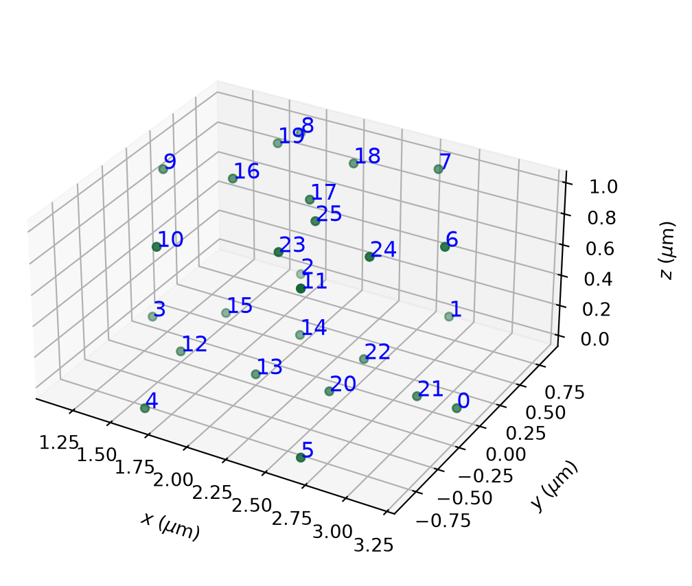
Each facet is given as a list of index rings: outer boundary first, then holes. Winding order sets the outward normal; hole rings wind opposite to their outer boundary so shapely subtracts them correctly.
facets = [None] * 15
facets[0] = [
[5, 4, 3, 2, 1, 0], # bottom cap (outward normal -z), hexagon reversed
[12, 13, 14, 15], # square hole
[20, 21, 22], # triangular hole
]
facets[1] = [
[6, 7, 8, 9, 10, 11], # top cap (outward normal +z)
[19, 18, 17, 16], # square hole (reversed to match the slant)
[25, 24, 23], # triangular hole (reversed)
]
facets[2] = [[0, 1, 7, 6]] # hexagon side wall
facets[3] = [[1, 2, 8, 7]]
facets[4] = [[2, 3, 9, 8]]
facets[5] = [[3, 4, 10, 9]]
facets[6] = [[4, 5, 11, 10]]
facets[7] = [[5, 0, 6, 11]]
facets[8] = [[12, 13, 17, 16]] # square hole inner wall
facets[9] = [[13, 14, 18, 17]]
facets[10] = [[14, 15, 19, 18]]
facets[11] = [[15, 12, 16, 19]]
facets[12] = [[20, 21, 24, 23]] # triangular hole inner wall
facets[13] = [[21, 22, 25, 24]]
facets[14] = [[22, 20, 23, 25]]Sanity-check the facet table: one outer ring plus any holes per facet.
for i, facet in enumerate(facets):
print(f"facet {i:2d}:")
for j, poly in enumerate(facet):
tag = "outer" if j == 0 else f"hole {j}"
print(f" {tag:8s} {poly}")facet 0:
outer [5, 4, 3, 2, 1, 0]
hole 1 [12, 13, 14, 15]
hole 2 [20, 21, 22]
facet 1:
outer [6, 7, 8, 9, 10, 11]
hole 1 [19, 18, 17, 16]
hole 2 [25, 24, 23]
facet 2:
outer [0, 1, 7, 6]
facet 3:
outer [1, 2, 8, 7]
facet 4:
outer [2, 3, 9, 8]
facet 5:
outer [3, 4, 10, 9]
facet 6:
outer [4, 5, 11, 10]
facet 7:
outer [5, 0, 6, 11]
facet 8:
outer [12, 13, 17, 16]
facet 9:
outer [13, 14, 18, 17]
facet 10:
outer [14, 15, 19, 18]
facet 11:
outer [15, 12, 16, 19]
facet 12:
outer [20, 21, 24, 23]
facet 13:
outer [21, 22, 25, 24]
facet 14:
outer [22, 20, 23, 25]Each facet is triangulated in its own 2D plane: _facet_basis fits a local basis, _to_2d/_to_3d convert coordinates, and shapely + trimesh.creation.triangulate_polygon triangulate the polygon-with-holes. The pieces are merged into one mesh with consistent normals.
from shapely.geometry import Polygon
def _facet_basis(pts, atol=1e-8):
"""Build an orthonormal (origin, u, v, normal) basis for a planar polygon.
Raises ValueError if pts are collinear or not (nearly) coplanar. The
tolerance is relative to the facet's own bounding-box diagonal, so it
scales correctly whether coordinates are in nm, um, or m.
"""
pts = np.asarray(pts, dtype=float)
p0 = pts[0]
u = pts[1] - p0
u = u / np.linalg.norm(u)
normal = None
for i in range(2, len(pts)):
n = np.cross(u, pts[i] - p0)
if np.linalg.norm(n) > 1e-12:
normal = n / np.linalg.norm(n)
break
if normal is None:
raise ValueError("facet points are collinear; cannot define a plane")
v = np.cross(normal, u)
rel = pts - p0
dist_from_plane = rel @ normal
scale = np.linalg.norm(pts.max(axis=0) - pts.min(axis=0))
scale = scale if scale > 0 else 1.0
max_dev = np.abs(dist_from_plane).max()
if max_dev > atol * scale:
bad = int(np.argmax(np.abs(dist_from_plane)))
raise ValueError(
f"facet points are not coplanar: point {bad} is {max_dev:.3e} off "
f"the plane (tolerance {atol * scale:.3e} for this facet's size)"
)
return p0, u, v, normal
def _to_2d(pts, p0, u, v):
rel = pts - p0
return np.column_stack([rel @ u, rel @ v])
def _to_3d(pts2d, p0, u, v):
return p0 + np.outer(pts2d[:, 0], u) + np.outer(pts2d[:, 1], v)
def planarsolid_to_trimesh(vtx, facets):
"""Triangulate a planar-solid facet table (0-based vertex indices, outer
boundary + optional hole rings per facet) into a trimesh.Trimesh."""
verts_out = []
faces_out = []
for facet in facets:
outer_pts = vtx[np.array(facet[0])]
p0, u, v, normal = _facet_basis(outer_pts)
outer_2d = _to_2d(outer_pts, p0, u, v)
holes_2d = [_to_2d(vtx[np.array(hole)], p0, u, v) for hole in facet[1:]]
poly = Polygon(outer_2d, holes_2d)
v2d, faces = trimesh.creation.triangulate_polygon(poly, engine="triangle")
v3d = _to_3d(v2d, p0, u, v)
offset = len(verts_out)
verts_out.extend(v3d)
faces_out.extend(faces + offset)
mesh = trimesh.Trimesh(vertices=np.array(verts_out), faces=np.array(faces_out))
mesh.merge_vertices()
mesh.fix_normals()
return meshBuild and visualize the mesh.
planarsolid_mesh = planarsolid_to_trimesh(vtx, facets)
planarsolid_mesh.show()Convert the mesh into a Tidy3D TriangleMesh and check both the cross sections and the 3D view of the resulting structure in Tidy3D.
planarsolid_geo = td.TriangleMesh.from_trimesh(planarsolid_mesh)
fig, (ax1, ax2) = plt.subplots(1, 2, tight_layout=True)
planarsolid_geo.plot(z=0.5, ax=ax1)
planarsolid_geo.plot(y=0, ax=ax2)
plt.show()
planarsolid_str = td.Structure(geometry=planarsolid_geo, medium=td.Medium())
scene = td.Scene(structures=[planarsolid_str])
scene.plot_3d()13:59:28 UTC WARNING: Plotting a 'TriangleMesh' may give inconsistent results if the mesh is not unionized. We recommend unionizing all meshes before import. A 'PermittivityMonitor' can be used to check that the mesh is loaded correctly.
WARNING: Plotting a 'TriangleMesh' may give inconsistent results if the mesh is not unionized. We recommend unionizing all meshes before import. A 'PermittivityMonitor' can be used to check that the mesh is loaded correctly.


 TERMS & CONDITIONS


 How the process works:
 Try this real URL to see an example: