





import matplotlib.pyplot as plt
import numpy as np
import tidy3d as td
import tidy3d.web as web
TIDY3D
LEARNING CENTER
Example Library

Integrated vector vortex beam generator
Note: the cost of running the entire notebook is larger than 10 FlexCredits.
A whispering-gallery mode of a microring is an angular-momentum eigenstate: the field varies as \(e^{im\theta}\), so every photon carries \(m\hbar\) of orbital angular momentum (OAM) about the ring axis. That momentum is trapped, because the azimuthal wavevector \(m/R_0 = k_0 n_\mathrm{eff}\) lies outside the free-space light cone. Etching \(q\) identical scattering elements into the ring breaks the continuous rotational symmetry down to a discrete \(q\)-fold one, so angular momentum is conserved only modulo \(q\). The mode can then shed \(q\) units and escape as a free-space beam of topological charge
\[\ell = m - q,\]
which is the angular phase-matching condition. Because every scatterer is an identical rotated copy, the emitted polarization rotates with the azimuthal coordinate as well, so the output is a vector vortex beam rather than a scalar one.
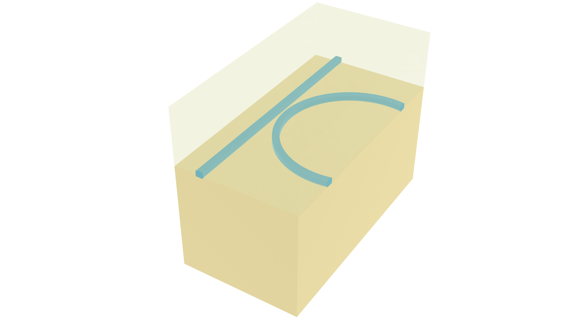
In this notebook, we reproduce the far-field emission of the vertically coupled device of S. A. Schulz, T. Machula, E. Karimi, and R. W. Boyd, “Integrated multi vector vortex beam generator,” Opt. Express 21, 16130-16141 (2013). A single ring of radius \(R_0 = 3.9\ \mu m\) is driven through a bus waveguide in a separate layer, 275 nm of silica below it. With \(m = 39\) at the design wavelength, gratings of \(q = 38\) and \(q = 37\) emit \(\ell = +1\) and \(\ell = +2\). The headline result is topological: the \(\ell = +2\) beam is a doughnut with a dark vortex core, while the \(\ell = +1\) beam has a bright core. A radially polarized beam of charge \(\ell\) splits into circular components of charge \(\ell - 1\) and \(\ell + 1\), and a charge-zero component is the only one that survives on axis — so \(\ell = \pm 1\) is the exception that fills the middle in. We measure 99.6% relative on-axis intensity for \(\ell = +1\) and 0.2% for \(\ell = +2\).
Moving the bus out of the ring’s plane frees the plane so that concentric rings can each be addressed by their own buried waveguide, which is what allows OAM qudit states to be synthesized on chip.

For more integrated photonic examples, please visit our examples page. If you are new to the finite-difference time-domain (FDTD) method, we highly recommend going through our FDTD101 tutorials.
Simulation Setup
The design wavelength is 1542 nm. We use a broad source so that several ring resonances appear in the bus spectrum, and record the far field on a narrower band bracketing the \(m = 39\) resonance.
lda0 = 1.542  # design wavelength (um)
freq0 = td.C_0 / lda0

ldas_wide = np.linspace(1.45, 1.65, 401)  # bus transmission spectrum
freqs_wide = td.C_0 / ldas_wide

ldas = np.linspace(1.522, 1.562, 41)  # far-field band around m = 39
freqs = td.C_0 / ldas

fwidth = 0.7 * (np.max(freqs_wide) - np.min(freqs_wide))
Both the ring and the bus are 220 nm thick and 500 nm wide silicon, encapsulated in silica, with the two silicon layers separated by 275 nm of oxide. The ring mode number at the design wavelength is \(m = 39\), so \(q = 38\) and \(q = 37\) give \(\ell = +1\) and \(\ell = +2\).
R0 = 3.9  # ring radius, i.e. the waveguide centreline (um)
w_wg = 0.5  # waveguide width
t_si = 0.22  # silicon layer thickness
t_sep = 0.275  # silica between the bus layer and the ring layer
t_top = 0.3  # silica over the ring

m_ring = 39  # ring mode number at lda0
q_values = [38, 37]  # grating element counts -> l = m - q = +1, +2

r_in, r_out = R0 - w_wg / 2, R0 + w_wg / 2

# layer stack, bottom to top: oxide | bus Si | 275 nm oxide | ring Si | 300 nm oxide | air
z_bus = (0.0, t_si)
z_ring = (t_si + t_sep, t_si + t_sep + t_si)
z_ox_top = z_ring[1] + t_top
y_bus = -R0  # the bus runs tangent to the ring, directly beneath the waveguide
The grating element size is the one dimension the source paper does not specify. Its radiation strength is set by the Fourier amplitude of the perturbation at the escaping order, which for rectangular teeth of azimuthal width \(w\) at pitch \(\Lambda\) scales as \(\sin(\pi w / \Lambda)\). A 60 nm wide tooth gives a loaded \(Q\) of about 2000, well above the 700-1000 quoted in the paper; widening it to 250 nm (\(w/\Lambda = 0.41\)) raises the radiated power roughly tenfold and brings \(Q\) into the reported range. Radial depth is the weaker knob, because the field outside the wall decays over roughly 124 nm. The extra silicon also shifts the \(m = 39\) resonance from 1542 nm to 1550 nm; that is 0.5%, which a 17 nm reduction of \(R_0\) would absorb and which sits below the two significant figures to which the radius is quoted, so we leave \(R_0 = 3.9\ \mu m\) as published rather than tuning it.
tooth_r = 0.06  # inward protrusion of a grating element
tooth_a = 0.25  # azimuthal width of a grating element
We use the dispersive crystalline silicon model from Tidy3D’s material library. Silica dispersion is negligible over this 200 nm band, so a constant index is used.
si = td.material_library["cSi"]["Li1993_293K"]
sio2 = td.Medium(permittivity=1.444**2)
The ring is an annulus with q teeth protruding inward from its inner wall, built as a GeometryGroup of a ClipOperation difference of two Cylinder objects plus one PolySlab per tooth. Each tooth overlaps the wall slightly so the union is watertight.
def grating_ring(q: int) -> td.Structure:
    """Ring annulus plus q grating teeth protruding inward from the inner wall."""
    annulus = td.Cylinder(
        center=(0, 0, np.mean(z_ring)), radius=r_out, length=t_si, axis=2
    ) - td.Cylinder(center=(0, 0, np.mean(z_ring)), radius=r_in, length=2 * t_si, axis=2)

    corners = np.array(
        [
            (r_in - tooth_r, -tooth_a / 2),
            (r_in + 0.01, -tooth_a / 2),
            (r_in + 0.01, tooth_a / 2),
            (r_in - tooth_r, tooth_a / 2),
        ]
    )
    teeth = []
    for j in range(q):
        angle = 2 * np.pi * j / q
        rot = np.array(
            [[np.cos(angle), -np.sin(angle)], [np.sin(angle), np.cos(angle)]]
        )
        teeth.append(
            td.PolySlab(vertices=corners @ rot.T, slab_bounds=z_ring, axis=2)
        )

    return td.Structure(
        geometry=td.GeometryGroup(geometries=[annulus, *teeth]), medium=si
    )


oxide = td.Structure(
    geometry=td.Box.from_bounds((-td.inf, -td.inf, -100), (td.inf, td.inf, z_ox_top)),
    medium=sio2,
)
bus = td.Structure(
    geometry=td.Box(center=(0, y_bus, np.mean(z_bus)), size=(td.inf, w_wg, t_si)),
    medium=si,
)
The domain is deliberately wide. The emitted beam is an annulus of radius \(R_0\) that keeps expanding, and a far-field projection is only meaningful if the collection plane captures essentially all of it — we verify this explicitly after the run.
Lx = Ly = 17.4  # domain size in x and y (um)
Lz, z_center = 4.5, 1.05
z_nf = 1.6  # collection plane, ~0.6 um above the top oxide
mon_size = 15.0  # collection plane extent (+-7.5 um)
x_port = 6.0
port_size = (0, 2.2, 1.8)
run_time = 15e-12
The quasi-TE mode of the bus is launched with a ModeSource. A FluxMonitor at the far end of the bus locates the resonances, a second one above the chip records the emitted power, and a FieldMonitor on the collection plane is used for the containment check.
The far field itself comes from a FieldProjectionAngleMonitor, which evaluates the Stratton-Chu integral on the server and returns the fields on any angular grid we choose. This is the right tool here: it samples the emission cone at whatever resolution we like without the windowing and aliasing that a discrete Fourier transform of a finite near-field plane would introduce.
def make_sim(q: int) -> td.Simulation:
    """Build the vertically coupled ring emitter with a q-element angular grating."""
    mode_source = td.ModeSource(
        center=(-x_port, y_bus, np.mean(z_bus)),
        size=port_size,
        source_time=td.GaussianPulse(freq0=freq0, fwidth=fwidth),
        direction="+",
        mode_spec=td.ModeSpec(num_modes=1, target_neff=2.5),
        mode_index=0,
    )
    thru_monitor = td.FluxMonitor(
        center=(x_port, y_bus, np.mean(z_bus)),
        size=port_size,
        freqs=freqs_wide,
        name="thru",
    )
    up_monitor = td.FluxMonitor(
        center=(0, 0, z_nf), size=(mon_size, mon_size, 0), freqs=freqs, name="up"
    )
    field_monitor = td.FieldMonitor(
        center=(0, 0, z_nf),
        size=(mon_size, mon_size, 0),
        freqs=freqs,
        fields=["Ex", "Ey", "Ez"],
        interval_space=(5, 5, 1),
        colocate=True,
        name="near",
    )
    far_monitor = td.FieldProjectionAngleMonitor(
        center=(0, 0, z_nf),
        size=(mon_size, mon_size, 0),
        freqs=freqs,
        theta=list(np.deg2rad(np.linspace(0, 25, 126))),
        phi=list(np.linspace(0, 2 * np.pi, 181)[:-1]),
        proj_distance=1e5,
        far_field_approx=True,
        name="far",
    )
    return td.Simulation(
        center=(0, 0, z_center),
        size=(Lx, Ly, Lz),
        grid_spec=td.GridSpec.auto(min_steps_per_wvl=30, wavelength=lda0),
        structures=[oxide, grating_ring(q), bus],
        sources=[mode_source],
        monitors=[thru_monitor, up_monitor, field_monitor, far_monitor],
        run_time=run_time,
        shutoff=1e-5,
        # The silicon bus crosses the x boundary, as a port must. A dispersive
        # medium inside a PML is numerically unstable, so x uses an Absorber;
        # the y and z boundaries see only oxide and air.
        boundary_spec=td.BoundarySpec(
            x=td.Boundary.absorber(), y=td.Boundary.pml(), z=td.Boundary.pml()
        ),
        medium=td.Medium(),  # air above the top oxide
    )


sims = {f"l{m_ring - q}": make_sim(q) for q in q_values}
Before submitting, we visualize the setup. The right-hand panel shows the vertical coupler: the bus sits directly beneath the ring waveguide, separated by 275 nm of silica.
fig, (ax1, ax2, ax3) = plt.subplots(1, 3, figsize=(15, 4), tight_layout=True)
sim = sims["l1"]
sim.plot(z=np.mean(z_ring), ax=ax1)
ax1.set_title("Ring layer")
sim.plot(x=0, ax=ax2)
ax2.set_title("Vertical stack")
sim.plot(x=0, ax=ax3)
ax3.set_xlim(-5.2, -2.6)
ax3.set_ylim(-0.35, 1.25)
ax3.set_title("Vertical coupler")
plt.show()
Verifying the ring mode number
Before running the full 3D simulation, we check the design analytically. The resonance condition \(R_0 = m \lambda / (2 \pi n_\mathrm{eff})\) fixes the effective index that the ring waveguide must have for \(m = 39\) at 1542 nm. We solve the bent-waveguide mode with a ModeSimulation locally, setting bend_radius=-R0 because the mode plane sits at \(y = -R_0\) while the centre of curvature is at the origin.
lda_scan = np.linspace(1.50, 1.60, 21)
mode_wg = td.Structure(
    geometry=td.Box(center=(0, -R0, np.mean(z_ring)), size=(td.inf, w_wg, t_si)),
    medium=si,
)
mode_bg = td.Simulation(
    center=(0, -R0, np.mean(z_ring)),
    size=(1.0, 4.0, 3.0),
    grid_spec=td.GridSpec.auto(min_steps_per_wvl=40, wavelength=lda0),
    structures=[oxide, mode_wg],
    run_time=1e-13,
    boundary_spec=td.BoundarySpec.all_sides(boundary=td.PML()),
    medium=td.Medium(),
)
mode_sim = td.ModeSimulation.from_simulation(
    simulation=mode_bg,
    plane=td.Box(center=(0, -R0, np.mean(z_ring)), size=(0, 4.0, 3.0)),
    mode_spec=td.ModeSpec(num_modes=1, target_neff=2.5, bend_radius=-R0, bend_axis=1),
    freqs=list(td.C_0 / lda_scan),
)
mode_data = mode_sim.run_local().modes

n_eff = mode_data.n_eff.isel(mode_index=0).values.real
n_required = m_ring * lda0 / (2 * np.pi * R0)
print(f"n_eff at {lda0} um       : {np.interp(lda0, lda_scan, n_eff):.4f}")
print(f"required for m = {m_ring}    : {n_required:.4f}")

m_of_lda = 2 * np.pi * R0 * n_eff / lda_scan
lda_res = np.interp(m_ring, m_of_lda[::-1], lda_scan[::-1])
print(f"predicted m = {m_ring} resonance: {lda_res * 1e3:.1f} nm (paper: 1542 nm)")
Unable to connect to flexcompute.com. Please make sure you have a working internet connection for license verification.20:50:25 UTC ERROR: Unable to connect to flexcompute.com. Please make sure you have a working internet connection for license verification.
             ERROR: Unable to connect to flexcompute.com. Please make sure you
             have a working internet connection for license verification.
20:50:26 UTC ERROR: Unable to connect to flexcompute.com. Please make sure you
             have a working internet connection for license verification.
n_eff at 1.542 um       : 2.4945
required for m = 39    : 2.4542
predicted m = 39 resonance: 1557.0 nm (paper: 1542 nm)
The mode solve reproduces the paper’s design point to better than 0.1%, so we submit the two simulations as a Batch. We first check the maximum FlexCredit cost; the run shuts off automatically once the field has decayed, so we are only billed for the effective run time.
batch = web.Batch(simulations=sims, folder_name="vector-vortex-beam")
cost = batch.estimate_cost()
20:50:58 UTC Maximum FlexCredit cost: 46.553 for the whole batch.
batch_data = batch.run(path_dir="data")20:50:59 UTC Started working on Batch containing 2 tasks.
Maximum FlexCredit cost: 46.553 for the whole batch.
             Use 'Batch.real_cost()' to get the billed FlexCredit cost after
             completion.
Postprocessing
Several ring resonances fall inside the recorded band, and they carry different topological charges because \(\ell = m - q\) changes with \(m\). Selecting the brightest peak would therefore compare two different modes, so instead we identify every resonance, measure its charge from the azimuthal Fourier spectrum of the far field, and keep the one that matches \(\ell = m - q\).
def azimuthal_charge(field: np.ndarray, n_modes: int = 1) -> list:
    """Dominant exp(i m phi) harmonics of a far-field component, as (m, weight)."""
    coeff = np.fft.fftshift(np.fft.fft(field, axis=-1), axes=-1) / field.shape[-1]
    orders = np.fft.fftshift(
        np.fft.fftfreq(field.shape[-1], 1 / field.shape[-1])
    ).astype(int)
    weight = (np.abs(coeff) ** 2).sum(axis=0)
    best = np.argsort(weight)[::-1][:n_modes]
    return [(int(orders[i]), weight[i] / weight.sum()) for i in best]


results = {}
for q in q_values:
    ell = m_ring - q
    sim_data = batch_data[f"l{ell}"]
    # monitor data is stored on its own frequency coordinate (ascending), so we
    # read wavelengths from the data rather than from the input array
    f_band = sim_data["up"].flux.f.values
    lda_band = td.C_0 / f_band * 1e3
    up = np.abs(sim_data["up"].flux.values)

    peaks = [
        k
        for k in range(1, len(up) - 1)
        if up[k] >= up[k - 1] and up[k] >= up[k + 1] and up[k] > 0.15 * up.max()
    ]
    charges = []
    for k in peaks:
        e_theta = (
            sim_data["far"]
            .Etheta.sel(f=f_band[k])
            .squeeze(drop=True)
            .transpose("theta", "phi")
            .values
        )
        charges.append((k, azimuthal_charge(e_theta)[0][0]))

    print(f"q = {q}: " + ", ".join(
        f"{lda_band[k]:.0f} nm -> l = {c:+d} (m = {c + q})" for k, c in charges
    ))
    k_res = [k for k, c in charges if c == ell][0]
    results[ell] = dict(
        freq=float(f_band[k_res]), lda=float(lda_band[k_res]), eta=float(up[k_res]),
        data=sim_data
    )
q = 38: 1527 nm -> l = +2 (m = 40), 1550 nm -> l = +1 (m = 39)
q = 37: 1526 nm -> l = +3 (m = 40), 1550 nm -> l = +2 (m = 39)The far field is only trustworthy if the collection plane actually contained the beam. We check the enclosed transverse intensity as a function of radius: the curve must flatten before the edge of the plane, otherwise the pattern would be dominated by diffraction from the truncated aperture rather than by the device.
for ell, res in results.items():
    near = res["data"]["near"]
    ex = near.Ex.sel(f=res["freq"]).squeeze(drop=True)
    ey = near.Ey.sel(f=res["freq"]).squeeze(drop=True)
    intensity = (np.abs(ex) ** 2 + np.abs(ey) ** 2).transpose("x", "y").values
    xx, yy = np.meshgrid(ex.x.values, ey.y.values, indexing="ij")
    radius = np.hypot(xx, yy)
    frac = [intensity[radius < r].sum() / intensity.sum() for r in (3, 5, 6, 7, 7.4)]
    print(f"l = {ell:+d}: enclosed intensity at r = 3/5/6/7/7.4 um -> "
          + ", ".join(f"{f:.1%}" for f in frac))
l = +1: enclosed intensity at r = 3/5/6/7/7.4 um -> 23.8%, 86.6%, 95.4%, 98.9%, 99.4%
l = +2: enclosed intensity at r = 3/5/6/7/7.4 um -> 29.0%, 90.8%, 96.6%, 99.0%, 99.5%We also extract the loaded quality factor from the bus transmission dip and the fraction of the launched power radiated upward.
for ell, res in results.items():
    thru_data = res["data"]["thru"].flux
    lda_thru = td.C_0 / thru_data.f.values * 1e3
    thru = np.abs(thru_data.values)
    baseline = np.median(thru)
    window = np.abs(lda_thru - res["lda"]) < 6
    depth = 1 - thru[window] / baseline
    above = lda_thru[window][depth > depth.max() / 2]
    q_factor = res["lda"] / (above.max() - above.min())
    print(f"l = {ell:+d}: resonance {res['lda']:.1f} nm, Q = {q_factor:.0f}, "
          f"dip depth {depth.max():.0%}, upward emission {res['eta']:.1%}")
l = +1: resonance 1550.0 nm, Q = 1033, dip depth 95%, upward emission 21.6%
l = +2: resonance 1550.0 nm, Q = 1033, dip depth 95%, upward emission 18.7%Result Visualization
The far-field intensity is the reproduction of Fig. 4 of the source paper. The \(\ell = +2\) beam is a doughnut whose main lobe sits on the predicted emission cone \(\sin\theta = \ell / (k_0 R_0)\), while the \(\ell = +1\) beam is brightest exactly on axis. The concentric rings around both are the Bessel diffraction pattern of the annular source.
fig, axes = plt.subplots(2, 2, figsize=(11, 9), tight_layout=True)
for col, ell in enumerate(sorted(results)):
    res = results[ell]
    far = res["data"]["far"]
    theta = far.Etheta.theta.values
    phi = far.Ephi.phi.values
    e_theta = far.Etheta.sel(f=res["freq"]).squeeze(drop=True).transpose("theta", "phi").values
    e_phi = far.Ephi.sel(f=res["freq"]).squeeze(drop=True).transpose("theta", "phi").values
    intensity = np.abs(e_theta) ** 2 + np.abs(e_phi) ** 2

    # close the azimuthal grid so the polar mesh has no seam at phi = 0
    phi_c = np.append(phi, phi[0] + 2 * np.pi)
    intensity_c = np.concatenate([intensity, intensity[:, :1]], axis=1)
    tt, pp = np.meshgrid(np.degrees(theta), phi_c, indexing="ij")
    ax = axes[0, col]
    ax.pcolormesh(tt * np.cos(pp), tt * np.sin(pp), intensity_c / intensity_c.max(),
                  cmap="magma", shading="gouraud")
    ax.set_aspect("equal")
    ax.set_xlabel(r"$\theta\cos\phi$ (deg)")
    ax.set_ylabel(r"$\theta\sin\phi$ (deg)")
    ax.set_title(rf"$q={m_ring - ell}$, $\ell={ell:+d}$, $\lambda={res['lda']:.0f}$ nm")

    ax = axes[1, col]
    ax.plot(np.degrees(theta), intensity.mean(axis=1) / intensity.max(), lw=1.5)
    ax.axvline(np.degrees(np.arcsin(abs(ell) * lda0 / (2 * np.pi * R0))),
               color="C1", ls="--", lw=1, label=r"$\sin^{-1}(\ell / k_0 R_0)$")
    ax.set_xlabel(r"$\theta$ (deg)")
    ax.set_ylabel("Normalized intensity")
    ax.set_ylim(0, 1.05)
    ax.grid(alpha=0.3)
    ax.legend()
plt.show()
Finally we quantify the topology. A radially polarized vector vortex of charge \(\ell\) decomposes in the circular basis as \(E_x \pm i E_y \propto e^{i(\ell \pm 1)\phi}\), so the two spin components carry orbital charges \(\ell - 1\) and \(\ell + 1\). A component of charge \(n\) vanishes on axis as \(r^{|n|}\) unless \(n = 0\), which is why only \(\ell = \pm 1\) produces a bright core.
print(f"{'l':>4} {'measured l':>11} {'charge(Ex+iEy)':>15} {'charge(Ex-iEy)':>15} {'on-axis':>9}")
for ell in sorted(results):
    res = results[ell]
    far = res["data"]["far"]
    phi = far.Ephi.phi.values
    e_theta = far.Etheta.sel(f=res["freq"]).squeeze(drop=True).transpose("theta", "phi").values
    e_phi = far.Ephi.sel(f=res["freq"]).squeeze(drop=True).transpose("theta", "phi").values
    intensity = np.abs(e_theta) ** 2 + np.abs(e_phi) ** 2

    e_x = e_theta * np.cos(phi)[None, :] - e_phi * np.sin(phi)[None, :]
    e_y = e_theta * np.sin(phi)[None, :] + e_phi * np.cos(phi)[None, :]
    on_axis = intensity[0].mean() / intensity.max()
    print(f"{ell:>+4d} {azimuthal_charge(e_theta)[0][0]:>+11d} "
          f"{azimuthal_charge(e_x + 1j * e_y)[0][0]:>+15d} "
          f"{azimuthal_charge(e_x - 1j * e_y)[0][0]:>+15d} {on_axis:>9.1%}")
l measured l charge(Ex+iEy) charge(Ex-iEy) on-axis
+1 +1 +2 +0 99.6%
+2 +2 +3 +1 0.2%The measured charges follow \(\ell \pm 1\) exactly, and the \(\ell = +1\) device produces a charge-zero circular component, which is precisely why its core is bright while the \(\ell = +2\) core is dark.
No matching results found.


 TERMS & CONDITIONS


 How the process works:
 Try this real URL to see an example: