Author: Donghee Lee, University of Seoul

This notebook designs and analyzes a compact silicon waveguide Bragg grating notch filter using Tidy3D FDTD. The device is a primitive for photonic integrated circuits (PICs), telecommunication and WDM systems, and photonic neural-network interconnects. A Bragg grating reflects a narrow wavelength band while transmitting nearby wavelengths, which makes it useful for wavelength-selective routing, filtering, and channel conditioning.

The simulation uses a 2D effective-index model of a corrugated waveguide, broadband ModeSource excitation, and ModeMonitor measurements of the forward and backward modal power. A small Batch sweeps the grating period, and a short convergence check compares results across grid resolutions.

For more advanced PIC examples, see the PIC components notebook and the waveguide grating coupler notebook.

Schematic of the silicon waveguide Bragg grating filter

Setup¶

If this is your first time using Tidy3D, please follow the Start Here guide to install the package and configure your API key.

[1]:

from pathlib import Path

import numpy as np
import pandas as pd
import matplotlib.pyplot as plt
from IPython.display import display, Image

import tidy3d as td
import tidy3d.web as web

# Keep repeated non-fatal geometry warnings from cluttering the notebook output.
td.config.logging_level = "ERROR"

print("Tidy3D version:", td.__version__)
print("NumPy version:", np.__version__)


DATA_DIR = Path("data_bragg_grating_filter")
DATA_DIR.mkdir(exist_ok=True)

SUMMARY_CSV = DATA_DIR / "bragg_period_sweep_summary.csv"
SPECTRUM_CSV = DATA_DIR / "bragg_period_sweep_spectra.csv"
CONV_CSV = DATA_DIR / "bragg_convergence_check.csv"
FIELD_PNG = DATA_DIR / "best_bragg_filter_field.png"
FIELD_HDF5 = DATA_DIR / "best_bragg_filter_field.hdf5"

Tidy3D version: 2.10.2
NumPy version: 2.4.4

Device Concept¶

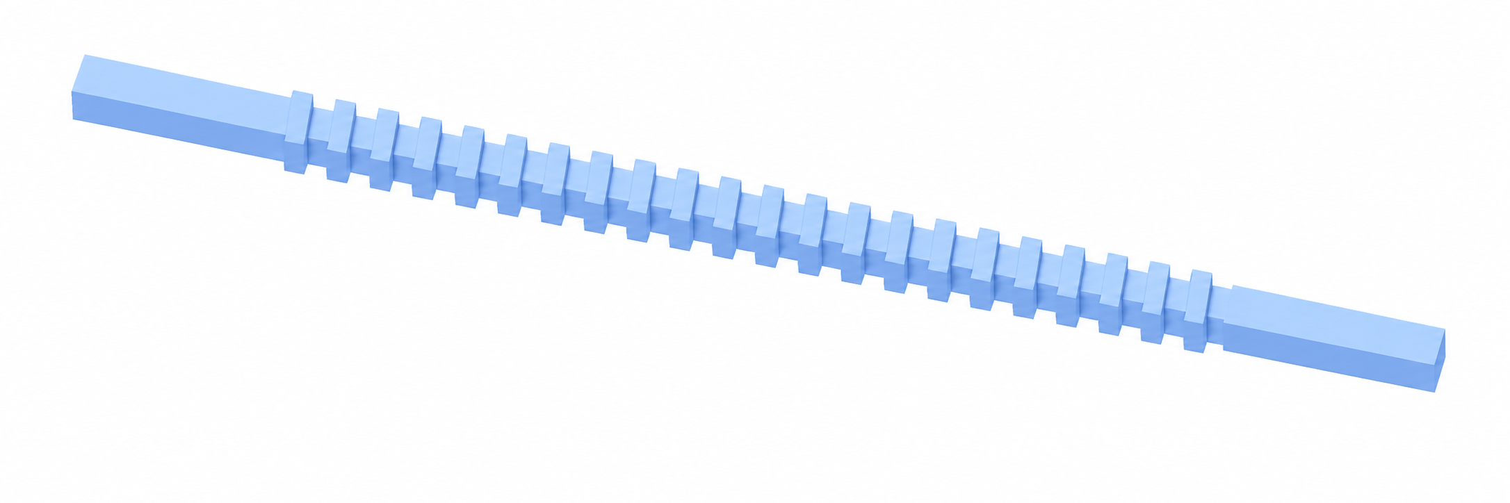
A waveguide Bragg grating consists of a periodic effective-index perturbation along a guided waveguide. Near the Bragg wavelength,

$$ \lambda_B \approx 2 n_{\mathrm{eff}} \Lambda, $$

the forward mode couples strongly into the backward mode, producing a reflection peak and a transmission notch.

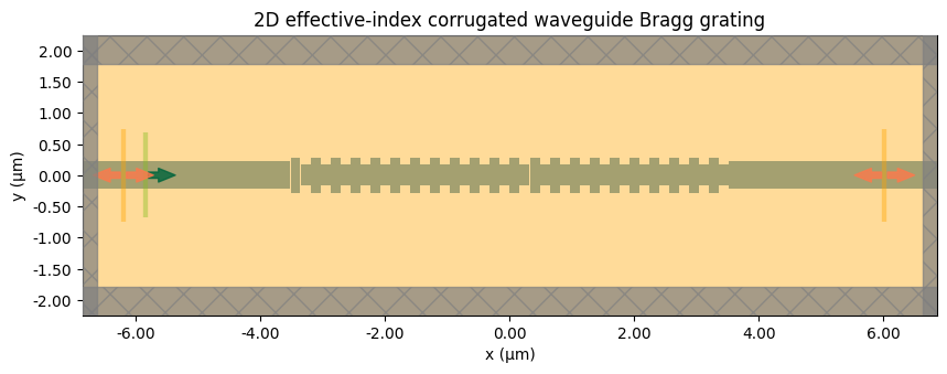
Here we use a 2D effective-index approximation, which captures the physics and the simulation workflow with a small computational footprint. The corrugation is implemented as alternating wider and narrower waveguide sections, defined as a list of Structure objects with Box geometries.

[2]:

# Units: Tidy3D uses micrometers for length.
um = 1.0

# Wavelength and frequency setup.
lambda_min = 1.50 * um
lambda_max = 1.60 * um
num_wavelengths = 101

# Use an ascending frequency grid. The corresponding wavelength grid will be descending.
wavelength_grid = np.linspace(lambda_min, lambda_max, num_wavelengths)
freq_grid_unsorted = td.C_0 / wavelength_grid
freqs = np.sort(freq_grid_unsorted)
wavelengths = td.C_0 / freqs

lambda0 = 1.55 * um
freq0 = td.C_0 / lambda0
fwidth = 0.10 * freq0

# 2D effective-index model.
# These are typical effective-index-like values, not a specific foundry stack.
n_core = 2.80
n_clad = 1.44

core = td.Medium(permittivity=n_core**2)
clad = td.Medium(permittivity=n_clad**2)

# Waveguide and grating geometry.
wg_width = 0.45 * um
corrugation_depth = 0.06 * um
num_periods = 22

input_len = 2.0 * um
output_len = 2.0 * um

# Simulation domain padding.
pad_x = 1.1 * um
pad_y = 1.5 * um

# Temporal and numerical settings.
min_steps_per_wvl_default = 28
run_time = 2.6e-12

# Compact Bragg-period sweep.
# Bragg estimate: lambda_B ≈ 2 n_eff Lambda. For lambda_B ~ 1.55 um and n_eff ~ 2.4,
# Lambda is around 0.32 um.
periods = np.linspace(0.300, 0.340, 5) * um

print("Wavelength grid [um]:", f"{wavelength_grid[0]:.3f} to {wavelength_grid[-1]:.3f}")
print("Number of Bragg periods per device:", num_periods)
print("Period sweep [um]:", np.round(periods, 4))

Wavelength grid [um]: 1.500 to 1.600
Number of Bragg periods per device: 22
Period sweep [um]: [0.3  0.31 0.32 0.33 0.34]

Simulation Setup¶

The function below builds a single 2D FDTD Simulation for a chosen grating period. A broadband ModeSource injects the fundamental guided mode at the input, and two ModeMonitor objects record the forward transmitted and backward reflected modal power. The grid is set with GridSpec.auto and the boundaries use PML on all sides.

[3]:

def make_bragg_sim(
    period,
    min_steps_per_wvl=min_steps_per_wvl_default,
    include_field_monitor=False,
):
    """Create a 2D effective-index Tidy3D simulation for a corrugated Bragg waveguide."""

    grating_length = num_periods * period
    x_total = input_len + grating_length + output_len + 2 * pad_x
    y_total = wg_width + 2 * corrugation_depth + 2 * pad_y

    x_grating_start = -grating_length / 2
    x_grating_end = +grating_length / 2

    x_left_wg_start = -x_total / 2 - pad_x  # extend input port through and past the PML
    x_source = -x_total / 2 + 0.70 * pad_x
    x_ref_monitor = -x_total / 2 + 0.38 * pad_x

    x_trans_monitor = x_total / 2 - 0.55 * pad_x
    x_right_wg_end = x_total / 2 + pad_x  # extend output port through and past the PML

    # Uniform input and output waveguide sections.
    structures = [
        td.Structure(
            geometry=td.Box(
                center=((x_left_wg_start + x_grating_start) / 2, 0, 0),
                size=(x_grating_start - x_left_wg_start, wg_width, td.inf),
            ),
            medium=core,
            name="input_waveguide",
        ),
        td.Structure(
            geometry=td.Box(
                center=((x_grating_end + x_right_wg_end) / 2, 0, 0),
                size=(x_right_wg_end - x_grating_end, wg_width, td.inf),
            ),
            medium=core,
            name="output_waveguide",
        ),
    ]

    # Corrugated grating: alternating wide and narrow half-period sections.
    # A small x-margin avoids exact contact between neighboring sub-cell boundaries
    # in the geometry validator while preserving the intended duty cycle.
    segment_margin = min(1e-3 * um, 0.02 * period)
    half_period = period / 2
    wide_width = wg_width + 2 * corrugation_depth
    narrow_width = wg_width - 2 * corrugation_depth

    for i in range(num_periods):
        x0 = x_grating_start + i * period

        wide_center = x0 + half_period / 2
        narrow_center = x0 + half_period + half_period / 2

        structures.append(
            td.Structure(
                geometry=td.Box(
                    center=(wide_center, 0, 0),
                    size=(half_period - segment_margin, wide_width, td.inf),
                ),
                medium=core,
                name=f"wide_{i:02d}",
            )
        )

        structures.append(
            td.Structure(
                geometry=td.Box(
                    center=(narrow_center, 0, 0),
                    size=(half_period - segment_margin, narrow_width, td.inf),
                ),
                medium=core,
                name=f"narrow_{i:02d}",
            )
        )

    pulse = td.GaussianPulse(freq0=freq0, fwidth=fwidth)
    mode_spec = td.ModeSpec(num_modes=1, target_neff=n_core)

    source = td.ModeSource(
        center=(x_source, 0, 0),
        size=(0, 2.4 * wide_width, td.inf),
        source_time=pulse,
        direction="+",
        mode_spec=mode_spec,
        mode_index=0,
        name="input_mode",
    )

    monitors = [
        td.ModeMonitor(
            center=(x_ref_monitor, 0, 0),
            size=(0, 2.6 * wide_width, td.inf),
            freqs=freqs,
            mode_spec=mode_spec,
            name="reflection_mode",
        ),
        td.ModeMonitor(
            center=(x_trans_monitor, 0, 0),
            size=(0, 2.6 * wide_width, td.inf),
            freqs=freqs,
            mode_spec=mode_spec,
            name="transmission_mode",
        ),
    ]

    if include_field_monitor:
        monitors.append(
            td.FieldMonitor(
                center=(0, 0, 0),
                size=(td.inf, td.inf, 0),
                freqs=[freq0],
                fields=["Ex", "Ey", "Ez"],
                name="field_xy",
            )
        )

    return td.Simulation(
        size=(x_total, y_total, 0),
        medium=clad,
        structures=structures,
        sources=[source],
        monitors=monitors,
        run_time=run_time,
        boundary_spec=td.BoundarySpec.all_sides(boundary=td.PML()),
        grid_spec=td.GridSpec.auto(min_steps_per_wvl=min_steps_per_wvl),
    )

Geometry Preview¶

Plot the 2D layout to confirm the grating geometry before submitting any cloud jobs.

[4]:

preview_sim = make_bragg_sim(periods[len(periods) // 2], include_field_monitor=True)

fig, ax = plt.subplots(figsize=(10, 3.6))
preview_sim.plot(z=0, ax=ax)
ax.set_title("2D effective-index corrugated waveguide Bragg grating")
plt.show()

No description has been provided for this image

Post-Processing Helpers¶

The helpers below extract the modal-power spectrum from each ModeMonitor, compute summary metrics for the Bragg filter, and assemble the per-period spectrum and summary tables.

[5]:

def extract_mode_power_spectrum(sim_data, monitor_name, direction, mode_index=0):
    """Extract |a|^2 spectrum from a Tidy3D ModeMonitor."""

    amp = (
        sim_data[monitor_name]
        .amps.sel(direction=direction, mode_index=mode_index)
        .values
    )
    return np.abs(np.asarray(amp).squeeze()) ** 2


def bragg_metrics(wavelength_um, transmission, reflection):
    """Return compact spectral metrics for a Bragg grating filter."""

    wavelength_um = np.asarray(wavelength_um)
    transmission = np.asarray(transmission)
    reflection = np.asarray(reflection)

    t_min_idx = int(np.argmin(transmission))
    r_max_idx = int(np.argmax(reflection))

    notch_wavelength_um = float(wavelength_um[t_min_idx])
    reflection_peak_wavelength_um = float(wavelength_um[r_max_idx])

    min_transmission = float(transmission[t_min_idx])
    max_reflection = float(reflection[r_max_idx])

    notch_depth_db = -10 * np.log10(max(min_transmission, 1e-30))

    # Combined score: high reflection, deep notch, center wavelength near 1.55 um.
    center_error_um = abs(reflection_peak_wavelength_um - 1.55)
    score = max_reflection - min_transmission - 2.0 * center_error_um

    return {
        "notch_wavelength_um": notch_wavelength_um,
        "reflection_peak_wavelength_um": reflection_peak_wavelength_um,
        "min_transmission": min_transmission,
        "max_reflection": max_reflection,
        "notch_depth_dB": float(notch_depth_db),
        "center_error_um": float(center_error_um),
        "filter_score": float(score),
    }


def summarize_bragg_batch(batch_results, task_meta, summary_csv, spectrum_csv):
    """Convert a completed Bragg-grating BatchData into summary and spectrum tables.

    task_meta maps each task name to a dict with keys ``period_um`` and
    ``min_steps_per_wvl``.
    """

    rows_summary = []
    rows_spectrum = []

    wl_um = np.asarray(td.C_0 / freqs)
    wl_order = np.argsort(wl_um)
    wl_sorted = wl_um[wl_order]

    for task_name in batch_results.keys():
        sim_data = batch_results[task_name]

        period_um = task_meta[task_name]["period_um"]
        resolution = task_meta[task_name].get("min_steps_per_wvl", np.nan)

        transmission = extract_mode_power_spectrum(sim_data, "transmission_mode", "+")
        reflection = extract_mode_power_spectrum(sim_data, "reflection_mode", "-")

        transmission = np.asarray(transmission)[wl_order]
        reflection = np.asarray(reflection)[wl_order]

        metrics = bragg_metrics(wl_sorted, transmission, reflection)

        rows_summary.append(
            {
                "task": task_name,
                "period_um": period_um,
                "min_steps_per_wvl": resolution,
                **metrics,
            }
        )

        for wl, t_val, r_val in zip(wl_sorted, transmission, reflection):
            rows_spectrum.append(
                {
                    "task": task_name,
                    "period_um": period_um,
                    "min_steps_per_wvl": resolution,
                    "wavelength_um": float(wl),
                    "transmission": float(t_val),
                    "reflection": float(r_val),
                }
            )

    summary_df = (
        pd.DataFrame(rows_summary).sort_values("period_um").reset_index(drop=True)
    )
    spectrum_df = (
        pd.DataFrame(rows_spectrum)
        .sort_values(["period_um", "wavelength_um"])
        .reset_index(drop=True)
    )

    summary_df.to_csv(summary_csv, index=False)
    spectrum_df.to_csv(spectrum_csv, index=False)

    return summary_df, spectrum_df

Bragg Period Sweep¶

Submit a small Batch of FDTD jobs covering five grating periods. If the cached CSV files already exist, the cell loads them instead of resubmitting.

[6]:

if SUMMARY_CSV.exists() and SPECTRUM_CSV.exists():
    summary_df = pd.read_csv(SUMMARY_CSV)
    spectrum_df = pd.read_csv(SPECTRUM_CSV)

else:
    sweep_sims = {
        f"P_{float(P):.3f}um": make_bragg_sim(P, include_field_monitor=False)
        for P in periods
    }
    sweep_meta = {
        name: {"period_um": float(P), "min_steps_per_wvl": min_steps_per_wvl_default}
        for name, P in zip(sweep_sims.keys(), periods)
    }

    bragg_batch_results = web.Batch(simulations=sweep_sims, verbose=True).run(
        path_dir=str(DATA_DIR / "sweep")
    )

    summary_df, spectrum_df = summarize_bragg_batch(
        batch_results=bragg_batch_results,
        task_meta=sweep_meta,
        summary_csv=SUMMARY_CSV,
        spectrum_csv=SPECTRUM_CSV,
    )

display(summary_df)

best_row = summary_df.sort_values("filter_score", ascending=False).iloc[0]
best_period = float(best_row["period_um"]) * um

print("\nBest Bragg grating design:")
display(best_row)
print(f"Best period = {best_period:.3f} um")

	task	period_um	min_steps_per_wvl	notch_wavelength_um	reflection_peak_wavelength_um	min_transmission	max_reflection	notch_depth_dB	center_error_um	filter_score
0	P_0.300um	0.30	28	1.515	1.511	0.126762	0.872484	8.970103	0.039	0.667722
1	P_0.310um	0.31	28	1.559	1.560	0.113829	0.884512	9.437475	0.010	0.750683
2	P_0.320um	0.32	28	1.600	1.599	0.102077	0.898692	9.910727	0.049	0.698615
3	P_0.330um	0.33	28	1.600	1.600	0.345951	0.651996	4.609856	0.050	0.206045
4	P_0.340um	0.34	28	1.592	1.592	0.862651	0.130350	0.641646	0.042	-0.816301

Best Bragg grating design:

task                             P_0.310um
period_um                             0.31
min_steps_per_wvl                       28
notch_wavelength_um                  1.559
reflection_peak_wavelength_um         1.56
min_transmission                  0.113829
max_reflection                    0.884512
notch_depth_dB                    9.437475
center_error_um                       0.01
filter_score                      0.750683
Name: 1, dtype: object

Best period = 0.310 um

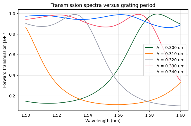
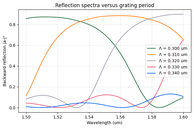
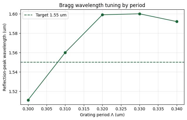
Spectrum Visualization¶

Plot the broadband transmission and reflection spectra for each grating period, and the Bragg-peak wavelength as a function of period. A useful filter shows a clear transmission notch and reflection peak near the target WDM wavelength.

[7]:

fig, ax = plt.subplots(figsize=(7.5, 4.5))

for period_um, group in spectrum_df.groupby("period_um"):
    ax.plot(
        group["wavelength_um"],
        group["transmission"],
        label=f"Λ = {period_um:.3f} um",
    )

ax.set_xlabel("Wavelength (um)")
ax.set_ylabel("Forward transmission |a+|²")
ax.set_title("Transmission spectra versus grating period")
ax.grid(True, alpha=0.3)
ax.legend()
plt.show()

fig, ax = plt.subplots(figsize=(7.5, 4.5))

for period_um, group in spectrum_df.groupby("period_um"):
    ax.plot(
        group["wavelength_um"],
        group["reflection"],
        label=f"Λ = {period_um:.3f} um",
    )

ax.set_xlabel("Wavelength (um)")
ax.set_ylabel("Backward reflection |a-|²")
ax.set_title("Reflection spectra versus grating period")
ax.grid(True, alpha=0.3)
ax.legend()
plt.show()

fig, ax = plt.subplots(figsize=(7.2, 4.2))
ax.plot(
    summary_df["period_um"], summary_df["reflection_peak_wavelength_um"], marker="o"
)
ax.axhline(1.55, linestyle="--", label="Target 1.55 um")
ax.set_xlabel("Grating period Λ (um)")
ax.set_ylabel("Reflection-peak wavelength (um)")
ax.set_title("Bragg wavelength tuning by period")
ax.grid(True, alpha=0.3)
ax.legend()
plt.show()

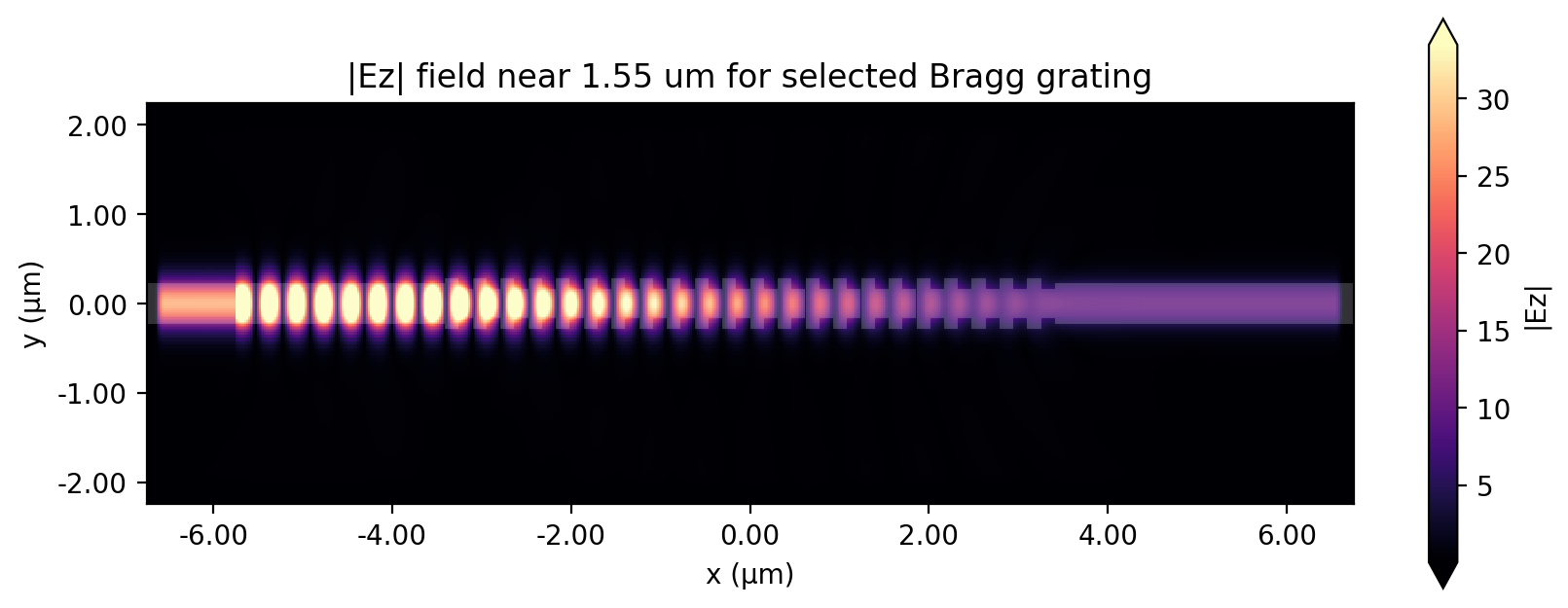
Field Plot for the Selected Design¶

The grating period that maximizes the filter score is rerun with a FieldMonitor to visualize the guided wave interacting with the corrugated region near the center wavelength.

[8]:

if FIELD_PNG.exists():
    print(f"Using cached field plot: {FIELD_PNG}")
    display(Image(filename=str(FIELD_PNG)))

else:
    best_sim = make_bragg_sim(
        best_period,
        min_steps_per_wvl=min_steps_per_wvl_default,
        include_field_monitor=True,
    )

    best_field_data = web.run(
        best_sim,
        task_name=f"best_bragg_P_{best_period:.3f}um_field",
        path=str(FIELD_HDF5),
        verbose=True,
    )

    fig, ax = plt.subplots(figsize=(10, 3.8))
    best_field_data.plot_field("field_xy", "Ez", val="abs", f=freq0, ax=ax)
    ax.set_title("|Ez| field near 1.55 um for selected Bragg grating")
    fig.savefig(FIELD_PNG, dpi=200, bbox_inches="tight")
    plt.show()

    print(f"Saved field plot to: {FIELD_PNG}")

Using cached field plot: data_bragg_grating_filter/best_bragg_filter_field.png

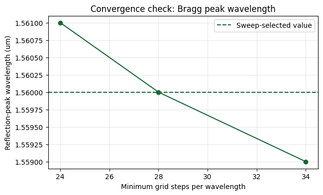
Short Convergence Check¶

A compact grid-resolution check on the selected design. The goal is not perfect numerical convergence but a sanity check that the spectral features do not shift dramatically with the grid step.

[9]:

if CONV_CSV.exists():
    conv_df = pd.read_csv(CONV_CSV)

else:
    conv_steps = [24, 28, 34]

    conv_sims = {
        f"P_{best_period:.3f}um_res_{steps}": make_bragg_sim(
            best_period,
            min_steps_per_wvl=steps,
            include_field_monitor=False,
        )
        for steps in conv_steps
    }
    conv_meta = {
        name: {"period_um": float(best_period), "min_steps_per_wvl": int(steps)}
        for name, steps in zip(conv_sims.keys(), conv_steps)
    }

    bragg_conv_batch_results = web.Batch(simulations=conv_sims, verbose=True).run(
        path_dir=str(DATA_DIR / "convergence")
    )

    conv_summary_df, _ = summarize_bragg_batch(
        batch_results=bragg_conv_batch_results,
        task_meta=conv_meta,
        summary_csv=DATA_DIR / "_tmp_bragg_convergence_summary.csv",
        spectrum_csv=DATA_DIR / "_tmp_bragg_convergence_spectra.csv",
    )

    conv_df = (
        conv_summary_df[
            [
                "min_steps_per_wvl",
                "period_um",
                "reflection_peak_wavelength_um",
                "notch_wavelength_um",
                "max_reflection",
                "min_transmission",
                "notch_depth_dB",
                "filter_score",
            ]
        ]
        .sort_values("min_steps_per_wvl")
        .reset_index(drop=True)
    )

    conv_df.to_csv(CONV_CSV, index=False)

display(conv_df)

fig, ax = plt.subplots(figsize=(7, 4))
ax.plot(
    conv_df["min_steps_per_wvl"], conv_df["reflection_peak_wavelength_um"], marker="o"
)
ax.axhline(
    best_row["reflection_peak_wavelength_um"],
    linestyle="--",
    label="Sweep-selected value",
)
ax.set_xlabel("Minimum grid steps per wavelength")
ax.set_ylabel("Reflection-peak wavelength (um)")
ax.set_title("Convergence check: Bragg peak wavelength")
ax.grid(True, alpha=0.3)
ax.legend()
plt.show()

	min_steps_per_wvl	period_um	reflection_peak_wavelength_um	notch_wavelength_um	max_reflection	min_transmission	notch_depth_dB	filter_score
0	24	0.31	1.561	1.559	0.884125	0.114291	9.419866	0.747834
1	28	0.31	1.560	1.559	0.884512	0.113829	9.437475	0.750683
2	34	0.31	1.559	1.558	0.885720	0.112461	9.489965	0.755259

Final Remarks¶

This notebook builds a 2D effective-index Bragg grating, sweeps the grating period, extracts wavelength-dependent transmission and reflection from mode monitors, selects a design near the target WDM wavelength, visualizes the field, and verifies the result with a short convergence check. The same workflow extends naturally to a 3D simulation of a foundry stack by replacing the effective-index slab with the full layer geometry and updating the materials accordingly.

TIDY3D
LEARNING CENTER

FDTD design of a silicon waveguide Bragg grating filter for WDM photonic circuits¶

Setup¶

Device Concept¶

Simulation Setup¶

Geometry Preview¶

Post-Processing Helpers¶

Bragg Period Sweep¶

Spectrum Visualization¶

Field Plot for the Selected Design¶

Short Convergence Check¶

Final Remarks¶

More Notebooks

TIDY3D LEARNING CENTER

FDTD design of a silicon waveguide Bragg grating filter for WDM photonic circuits¶

Setup¶

Device Concept¶

Simulation Setup¶

Geometry Preview¶

Post-Processing Helpers¶

Bragg Period Sweep¶

Spectrum Visualization¶

Field Plot for the Selected Design¶

Short Convergence Check¶

Final Remarks¶

More Notebooks

Cookie preferences

Privacy choices

TIDY3D
LEARNING CENTER