





Author: Haneul Lee, Korea Advanced Institute of Science and Technology
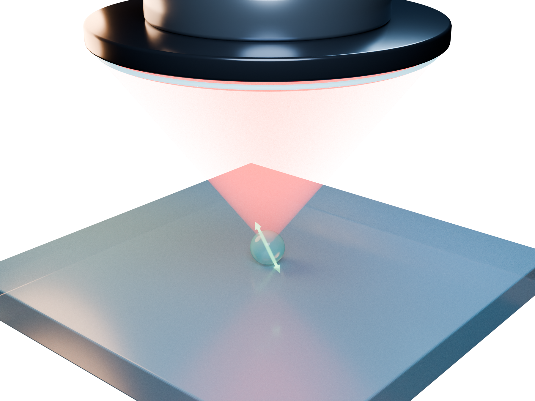
This notebook evaluates the fluorescence collection efficiency of diamond NV centers through a microscope objective for the following geometries:
- A spherical nanodiamond on a silica substrate
- A bulk-diamond NV center located beneath a planar air–diamond interface
- An NV center embedded in a finite-thickness diamond film on a silica substrate
The primary parameters investigated through systematic sweeps are:
- Nanodiamond diameter
- Polar and azimuthal orientations of the NV symmetry axis
- NV depth below the surface or position within the nanodiamond
- Emission wavelength
- Mesh spacing and near-to-far-field projection area
This notebook is developed using the official Tidy3D API from the 2.12 release series. Throughout the simulations, Tidy3D uses µm for length, Hz for frequency, and s for time.
Cloud execution and cost: Cells that call
run_batch_with_cost_estimate(...)first print the maximum estimated cost and then submit the batch to the Tidy3D cloud. Run the baseline and convergence stages selectively rather than using Run All, and review the task count printed by each stage before executing its batch cell.
0. Modeling Preliminaries
Distinction Between Established Facts and Modeling Assumptions
Facts Supported by the Literature and Tidy3D API
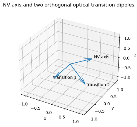
- The optical emission of an NV center is not modeled as a single dipole oriented along the NV symmetry axis. Instead, it is represented by two mutually orthogonal optical transition dipoles lying in the plane perpendicular to the NV symmetry axis.
- A three-dimensional Tidy3D
FluxMonitorenclosing the source integrates the net outward electromagnetic power flux through the closed monitoring surface. - A
FieldProjectionAngleMonitorprojects the recorded near-field distribution into specified far-field angular directions parameterized by $(\theta,\phi)$. - When an open projection surface is used for near-to-far-field transformation, convergence with respect to the projection-surface size must be verified. In particular, the projection boundary should be placed sufficiently far from the region of significant near-field amplitude so that truncation of the recorded field does not appreciably affect the projected far field.
Initial Modeling Assumptions Used in This Notebook
- The nanodiamond is assumed to be a perfect sphere.
- Diamond and silica are treated as isotropic, linear, nonmagnetic, and lossless dielectric materials.
- The NV center is modeled as a point electric dipole emitter.
- Unless otherwise specified, the NV center is assumed to be located at the center of the nanodiamond.
- The optical axis of the microscope objective is assumed to coincide with the surface normal, defined as the $+z$ direction.
- The silica substrate surface is assumed to be perfectly planar and laterally infinite.
If experimentally relevant effects such as the actual AFM/SEM-derived nanodiamond morphology, crystallographic faceting, the true spatial offset of the NV center within the nanodiamond, surface layers, material absorption, or surface roughness become important, the corresponding geometry and/or material models should be replaced accordingly while retaining the overall simulation framework.
Physical Quantity of Interest
Consider a microscope objective located on the air side, collecting radiation in the $+z$ direction. Let the refractive index of the medium on the objective side be $n_{\mathrm{obj}}$. The maximum polar angle accepted by an objective with numerical aperture $\mathrm{NA}$ is
$$ \theta_{\max} = \sin^{-1}\!\left( \frac{\mathrm{NA}}{n_{\mathrm{obj}}} \right). $$
If the far-field angular radiation intensity is expressed as
$$ \frac{dP}{d\Omega}(\theta,\phi,\lambda), $$
the optical power collected within the numerical aperture of the objective is
$$ P_{\mathrm{NA}}(\lambda) = \int_{0}^{2\pi} \int_{0}^{\theta_{\max}} \frac{dP}{d\Omega}(\theta,\phi,\lambda) \sin\theta \, d\theta \, d\phi. $$
Let $P_{\mathrm{tot}}(\lambda)$ denote the total radiated power obtained by integrating the electromagnetic power flux through a closed flux-monitor box surrounding the emitter. The fluorescence collection efficiency is then defined as
$$ \boxed{ \eta_{\mathrm{coll}}(\lambda) = \frac{ P_{\mathrm{NA}}(\lambda) }{ P_{\mathrm{tot}}(\lambda) } }. $$
The quantity $\eta_{\mathrm{coll}}$ represents the fraction of the total electromagnetic power radiated by the emitter that falls within the angular acceptance cone of the objective and can therefore reach its entrance pupil.
This definition does not include the following experimental losses or efficiencies:
- Objective transmission
- Dichroic-mirror and spectral-filter transmission
- Detector quantum efficiency
- Fiber-mode overlap and fiber-coupling efficiency
- Internal quantum efficiency of the NV center
- Nonradiative quenching associated with surfaces or interfaces
- Aberrations of the actual microscope objective
- Finite-pupil apodization and other pupil-dependent transmission effects
Therefore, $\eta_{\mathrm{coll}}$ should not be interpreted as the overall photon-detection efficiency of the experimental setup. To predict the experimentally measured photon count rate, the relevant optical transmission factors, detector response, and emitter quantum efficiency must be incorporated separately.
1. Prerequisites and Setup
Using the Tidy3D cloud solver requires a Flexcompute account and a valid API key; see the Get Started page for installation and authentication instructions.
The cell below imports the required packages and sets up the results directory for simulation outputs.
import json
from collections.abc import Mapping
from dataclasses import asdict, dataclass, replace
from pathlib import Path
from typing import Literal

import matplotlib.pyplot as plt
import numpy as np
import pandas as pd
import tidy3d as td
from IPython.display import display
from tidy3d import web

td.config.local_cache.enabled = False

RESULTS_DIR = Path("tidy3d_nv_results")
RESULTS_DIR.mkdir(parents=True, exist_ok=True)
RESULT_SET_TAG = "domain8_air1p4_film_absorber40"


def result_dir(stage_name: str) -> Path:
    """Return a settings-tagged directory so incompatible checkpoints cannot mix."""
    return RESULTS_DIR / f"{stage_name}_{RESULT_SET_TAG}"


print("Tidy3D version:", td.__version__)
print("Result directory:", RESULTS_DIR)
Tidy3D version: 2.12.0
Result directory: tidy3d_nv_results
2. Objective Acceptance Cone and Optical Constants
2.1 Acceptance Angle for an Objective with NA = 0.6
For a dry objective operating in air, $n_{\mathrm{obj}} = 1$. Therefore, the maximum collection angle is
$$ \theta_{\max} = \sin^{-1}\!\left(\frac{\mathrm{NA}}{n_{\mathrm{obj}}}\right) = \sin^{-1}(0.6) = 36.87^\circ. $$
Throughout this notebook, the $+z$ direction is defined as the direction toward the microscope objective.
OBJECTIVE_NA = 0.60
COLLECTION_INDEX = 1.0

if OBJECTIVE_NA > COLLECTION_INDEX:
    raise ValueError("NA must not exceed the collection-medium refractive index.")

theta_objective_rad = np.arcsin(OBJECTIVE_NA / COLLECTION_INDEX)
theta_objective_deg = np.degrees(theta_objective_rad)
print(f"Objective half-angle = {theta_objective_deg:.6f} deg")
Objective half-angle = 36.869898 deg
2.2 Refractive Indices of Diamond and Silica
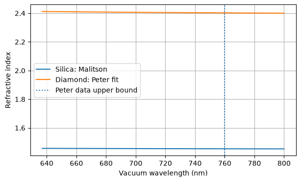
For silica, the refractive index is calculated using the Malitson Sellmeier equation for fused silica [1]:
$$ n^2 - 1 = \frac{0.6961663\lambda^2}{\lambda^2 - 0.0684043^2} + \frac{0.4079426\lambda^2}{\lambda^2 - 0.1162414^2} + \frac{0.8974794\lambda^2}{\lambda^2 - 9.896161^2}, $$
where the wavelength $\lambda$ is expressed in $\mathrm{\mu m}$.
For diamond, the refractive index is calculated using the Peter diamond Sellmeier equation [2]:
$$ n^2 - 1 = \frac{0.3306\lambda^2}{\lambda^2 - 0.1750^2} + \frac{4.3356\lambda^2}{\lambda^2 - 0.1060^2}, $$
where $\lambda$ is also expressed in $\mathrm{\mu m}$.
The reported validity range of the Peter refractive-index data extends to approximately 760 nm. Therefore, refractive-index values evaluated at wavelengths longer than 760 nm are treated as extrapolations of the Sellmeier model and should be interpreted accordingly.
SILICA_MALITSON_COEFFS = (
    (0.6961663, 0.0684043**2),
    (0.4079426, 0.1162414**2),
    (0.8974794, 9.896161**2),
)

DIAMOND_PETER_COEFFS = (
    (0.3306, 0.1750**2),
    (4.3356, 0.1060**2),
)

AIR = td.Medium(permittivity=1.0, name="air")
SILICA = td.Sellmeier(coeffs=SILICA_MALITSON_COEFFS, name="silica_malitson")
DIAMOND_PETER = td.Sellmeier(coeffs=DIAMOND_PETER_COEFFS, name="diamond_peter")


def sellmeier_n(
    wavelength_um: np.ndarray, coeffs: tuple[tuple[float, float], ...]
) -> np.ndarray:
    """Evaluate n(lambda) for Tidy3D-style Sellmeier coefficients (B_i, C_i)."""
    wavelength_um = np.asarray(wavelength_um, dtype=float)
    lam2 = wavelength_um**2
    n2 = np.ones_like(wavelength_um)
    for b_i, c_i in coeffs:
        n2 += b_i * lam2 / (lam2 - c_i)
    return np.sqrt(n2)


wvl_plot_nm = np.linspace(637.0, 800.0, 300)
wvl_plot_um = 1e-3 * wvl_plot_nm

fig, ax = plt.subplots(figsize=(7, 4))
ax.plot(
    wvl_plot_nm,
    sellmeier_n(wvl_plot_um, SILICA_MALITSON_COEFFS),
    label="Silica: Malitson",
)
ax.plot(
    wvl_plot_nm,
    sellmeier_n(wvl_plot_um, DIAMOND_PETER_COEFFS),
    label="Diamond: Peter fit",
)
ax.axvline(760.0, linestyle=":", label="Peter data upper bound")
ax.set_xlabel("Vacuum wavelength (nm)")
ax.set_ylabel("Refractive index")
ax.grid(True)
ax.legend()
plt.show()
3. NV Symmetry Axis and Two Optical Transition Dipoles
Let the polar and azimuthal angles of the NV symmetry axis be denoted by $\beta$ and $\alpha$, respectively. The corresponding unit vector is
$$ \hat{\mathbf{u}}_{\mathrm{NV}} = \left( \sin\beta\cos\alpha,\; \sin\beta\sin\alpha,\; \cos\beta \right). $$
The two optical transition dipoles, $\hat{\mathbf{e}}_1$ and $\hat{\mathbf{e}}_2$, are constructed such that both are perpendicular to the NV symmetry axis and mutually orthogonal:
$$ \hat{\mathbf{e}}_1 \cdot \hat{\mathbf{u}}_{\mathrm{NV}} = 0, \qquad \hat{\mathbf{e}}_2 \cdot \hat{\mathbf{u}}_{\mathrm{NV}} = 0, \qquad \hat{\mathbf{e}}_1 \cdot \hat{\mathbf{e}}_2 = 0. $$
Because the two optical transitions are treated as mutually incoherent, they are simulated independently and their radiated powers are summed at the power level.
The resulting NV-center collection efficiency is therefore defined as
$$ \eta_{\mathrm{NV}} = \frac{ P_{\mathrm{NA},1} + P_{\mathrm{NA},2} }{ P_{\mathrm{tot},1} + P_{\mathrm{tot},2} }. $$
In general, the arithmetic mean of the individual collection efficiencies,
$$ \frac{\eta_1+\eta_2}{2}, $$
is not equivalent to the expression above when the total radiated powers of the two transitions differ. The physically relevant quantity is the ratio of the sum of the collected powers to the sum of the total radiated powers.
def unit_vector_from_angles(beta_deg: float, alpha_deg: float) -> np.ndarray:
    """Polar beta is measured from +z; azimuth alpha is measured from +x toward +y."""
    beta = np.deg2rad(beta_deg)
    alpha = np.deg2rad(alpha_deg)
    return np.array(
        [np.sin(beta) * np.cos(alpha), np.sin(beta) * np.sin(alpha), np.cos(beta)],
        dtype=float,
    )


def nv_transition_basis(
    beta_deg: float, alpha_deg: float
) -> tuple[np.ndarray, np.ndarray, np.ndarray]:
    """Return NV axis u and a robust orthonormal transition-dipole basis e1, e2."""
    u_nv = unit_vector_from_angles(beta_deg, alpha_deg)
    u_nv /= np.linalg.norm(u_nv)

    z_hat = np.array([0.0, 0.0, 1.0])
    x_hat = np.array([1.0, 0.0, 0.0])
    reference = z_hat if abs(np.dot(u_nv, z_hat)) < 0.90 else x_hat

    e1 = np.cross(u_nv, reference)
    e1 /= np.linalg.norm(e1)
    e2 = np.cross(u_nv, e1)
    e2 /= np.linalg.norm(e2)
    return u_nv, e1, e2


def vector_to_spherical_angles(vector: np.ndarray) -> tuple[float, float]:
    """Return Tidy3D polar and azimuth angles in radians for a Cartesian direction."""
    vector = np.asarray(vector, dtype=float)
    vector /= np.linalg.norm(vector)
    theta = np.arccos(np.clip(vector[2], -1.0, 1.0))
    phi = np.mod(np.arctan2(vector[1], vector[0]), 2 * np.pi)
    return float(theta), float(phi)


u_test, e1_test, e2_test = nv_transition_basis(beta_deg=54.7356, alpha_deg=0.0)
G = np.array(
    [
        [np.dot(u_test, u_test), np.dot(u_test, e1_test), np.dot(u_test, e2_test)],
        [np.dot(e1_test, u_test), np.dot(e1_test, e1_test), np.dot(e1_test, e2_test)],
        [np.dot(e2_test, u_test), np.dot(e2_test, e1_test), np.dot(e2_test, e2_test)],
    ]
)

fig = plt.figure(figsize=(6, 5))
ax = fig.add_subplot(111, projection="3d")
origin = np.zeros(3)
for vector, label in [
    (u_test, "NV axis"),
    (e1_test, "transition 1"),
    (e2_test, "transition 2"),
]:
    ax.quiver(*origin, *vector, length=1.0, normalize=True)
    ax.text(*(1.08 * vector), label)
ax.set_xlim(-1.2, 1.2)
ax.set_ylim(-1.2, 1.2)
ax.set_zlim(-1.2, 1.2)
ax.set_xlabel("x")
ax.set_ylabel("y")
ax.set_zlabel("z")
ax.set_title("NV axis and two orthogonal optical transition dipoles")
plt.show()
4. Simulation Conditions and Geometry
The coordinate convention used throughout this notebook is defined as follows:
- Planar sample surface:
z = 0 - Microscope objective: located in the $+z$ direction
- Nanodiamond geometry: a spherical nanodiamond in contact with the silica substrate
- Bulk-diamond geometry: the entire half-space $z < 0$ is occupied by diamond
- Diamond-film geometry: the region $-t_{\mathrm{film}} < z < 0$ is occupied by diamond, with silica underneath
The parameter nv_depth_nm denotes the depth of the NV center measured downward from the top surface in the bulk-diamond and diamond-film geometries.
The parameter nv_offset_nm denotes the displacement of the NV center relative to the center of the nanodiamond in the nanodiamond geometry.
GeometryKind = Literal["nanodiamond", "bulk_halfspace", "diamond_film"]
DiamondModel = Literal["peter_sellmeier"]

# Large lateral reference domain used by the physical sweeps. The PML is
# added outside this non-PML domain by Tidy3D.
LARGE_DOMAIN_XY_SPAN_UM = 8.0
LARGE_PROJECTION_SPAN_UM = 4.8
# Half a wavelength is a hard construction guard, not a convergence claim.
# The baseline below targets about two wavelengths of lateral clearance at 700 nm.
MIN_PML_CLEARANCE_WAVELENGTHS = 0.5

@dataclass(frozen=True)
class ModelConfig:
    geometry: GeometryKind = "nanodiamond"
    wavelengths_nm: tuple[float, ...] = (700.0,)

    objective_na: float = 0.60
    collection_index: float = 1.0

    nd_diameter_nm: float = 40.0
    nd_embed_nm: float = 0.0
    nv_offset_nm: tuple[float, float, float] = (0.0, 0.0, 0.0)

    nv_depth_nm: float = 20.0
    film_thickness_nm: float = 500.0

    nv_beta_deg: float = 54.7356
    nv_alpha_deg: float = 0.0

    diamond_model: DiamondModel = "peter_sellmeier"

    mesh_dl_nm: float = 5.0
    min_steps_per_wvl: int = 20

    xy_span_um: float = LARGE_DOMAIN_XY_SPAN_UM
    air_buffer_um: float = 1.40
    substrate_buffer_um: float = 0.80

    projection_gap_um: float = 0.15
    projection_span_um: float = LARGE_PROJECTION_SPAN_UM
    projection_distance_um: float = 1000.0
    far_theta_max_deg: float = 80.0
    n_theta: int = 81
    n_phi: int = 181

    run_time_s: float = 2e-13
    shutoff: float = 1e-6
    film_absorber_num_layers: int = 40


def nm_to_um(value_nm: float | np.ndarray) -> float | np.ndarray:
    return 1e-3 * np.asarray(value_nm)


def get_diamond_medium(cfg: ModelConfig):
    if cfg.diamond_model == "peter_sellmeier":
        if max(cfg.wavelengths_nm) > 760.0:
            print(
                "WARNING: Peter diamond dispersion is being extrapolated above 760 nm."
            )
        return DIAMOND_PETER
    raise ValueError(f"Unknown diamond model: {cfg.diamond_model}")


def validate_config(cfg: ModelConfig) -> None:
    if not cfg.wavelengths_nm or min(cfg.wavelengths_nm) <= 0:
        raise ValueError("wavelengths_nm must contain positive values.")
    if not (0 < cfg.objective_na <= cfg.collection_index):
        raise ValueError("Require 0 < objective_na <= collection_index.")
    if cfg.far_theta_max_deg <= np.degrees(
        np.arcsin(cfg.objective_na / cfg.collection_index)
    ):
        raise ValueError(
            "far_theta_max_deg must exceed the objective acceptance angle."
        )
    if cfg.projection_span_um >= cfg.xy_span_um:
        raise ValueError("projection_span_um must be smaller than xy_span_um.")
    longest_wavelength_um = 1e-3 * max(cfg.wavelengths_nm)
    minimum_clearance_um = MIN_PML_CLEARANCE_WAVELENGTHS * longest_wavelength_um
    lateral_monitor_buffer = 0.5 * (cfg.xy_span_um - cfg.projection_span_um)
    if lateral_monitor_buffer < minimum_clearance_um - 1e-12:
        raise ValueError(
            f"Require at least {MIN_PML_CLEARANCE_WAVELENGTHS:g} times the longest "
            "vacuum wavelength between each projection-plane edge and the lateral PML start."
        )
    vertical_monitor_buffer = cfg.air_buffer_um - cfg.projection_gap_um
    if vertical_monitor_buffer < minimum_clearance_um - 1e-12:
        raise ValueError(
            f"Require at least {MIN_PML_CLEARANCE_WAVELENGTHS:g} times the longest "
            "vacuum wavelength between the projection plane and the +z PML start."
        )
    if cfg.mesh_dl_nm <= 0:
        raise ValueError("mesh_dl_nm must be positive.")
    if cfg.film_absorber_num_layers <= 0:
        raise ValueError("film_absorber_num_layers must be positive.")

    if cfg.geometry == "nanodiamond":
        radius_nm = 0.5 * cfg.nd_diameter_nm
        if radius_nm <= 0:
            raise ValueError("nd_diameter_nm must be positive.")
        if not (0 <= cfg.nd_embed_nm < cfg.nd_diameter_nm):
            raise ValueError("Require 0 <= nd_embed_nm < nd_diameter_nm.")
        if np.linalg.norm(np.asarray(cfg.nv_offset_nm, dtype=float)) >= radius_nm:
            raise ValueError(
                "The NV offset must remain inside the spherical nanodiamond."
            )
    elif cfg.geometry == "bulk_halfspace":
        if cfg.nv_depth_nm <= 0:
            raise ValueError("nv_depth_nm must be positive for bulk_halfspace.")
    elif cfg.geometry == "diamond_film":
        if cfg.film_thickness_nm <= 0:
            raise ValueError("film_thickness_nm must be positive.")
        if not (0 < cfg.nv_depth_nm < cfg.film_thickness_nm):
            raise ValueError(
                "For diamond_film, require 0 < nv_depth_nm < film_thickness_nm."
            )
    else:
        raise ValueError(f"Unknown geometry: {cfg.geometry}")


def wavelength_frequency_arrays(cfg: ModelConfig) -> tuple[np.ndarray, np.ndarray]:
    wavelengths_um = 1e-3 * np.asarray(cfg.wavelengths_nm, dtype=float)
    freqs = np.sort(td.C_0 / wavelengths_um)
    return wavelengths_um, freqs
Extend planar substrate geometries well beyond the nominal simulation domain so that they pass completely through the -z PML. This does not enlarge the FDTD computational domain.
PML_STRUCTURE_EXTENSION_UM = 2.0


def build_geometry(cfg: ModelConfig) -> dict:
    """Construct structures and return useful geometric coordinates."""
    validate_config(cfg)
    diamond = get_diamond_medium(cfg)
    xy_span = max(cfg.xy_span_um, cfg.projection_span_um + 0.35)

    structures = []

    if cfg.geometry == "nanodiamond":
        radius = 0.5 * float(nm_to_um(cfg.nd_diameter_nm))
        embed = float(nm_to_um(cfg.nd_embed_nm))
        sphere_center_z = radius - embed
        sphere_bottom_z = sphere_center_z - radius
        sphere_top_z = sphere_center_z + radius

        z_min = -max(cfg.substrate_buffer_um, abs(sphere_bottom_z) + 0.50)
        z_max = sphere_top_z + cfg.air_buffer_um
        z_structure_min = z_min - PML_STRUCTURE_EXTENSION_UM

        substrate = td.Structure(
            geometry=td.Box(
                center=(0.0, 0.0, 0.5 * z_structure_min),
                size=(td.inf, td.inf, -z_structure_min),
            ),
            medium=SILICA,
            name="silica_substrate",
        )
        sphere = td.Structure(
            geometry=td.Sphere(center=(0.0, 0.0, sphere_center_z), radius=radius),
            medium=diamond,
            name="nanodiamond",
        )
        # Later structures override earlier structures in overlap regions.
        structures.extend([substrate, sphere])

        offset_um = np.asarray(cfg.nv_offset_nm, dtype=float) * 1e-3
        nv_position = np.array([0.0, 0.0, sphere_center_z]) + offset_um
        object_top_z = sphere_top_z
        object_bottom_z = min(0.0, sphere_bottom_z)

    elif cfg.geometry == "bulk_halfspace":
        depth = float(nm_to_um(cfg.nv_depth_nm))
        z_min = -max(cfg.substrate_buffer_um, depth + 0.60)
        z_max = cfg.air_buffer_um
        z_structure_min = z_min - PML_STRUCTURE_EXTENSION_UM
        bulk = td.Structure(
            geometry=td.Box(
                center=(0.0, 0.0, 0.5 * z_structure_min),
                size=(td.inf, td.inf, -z_structure_min),
            ),
            medium=diamond,
            name="bulk_diamond",
        )
        structures.append(bulk)
        nv_position = np.array([0.0, 0.0, -depth])
        object_top_z = 0.0
        object_bottom_z = z_min

    elif cfg.geometry == "diamond_film":
        film_thickness = float(nm_to_um(cfg.film_thickness_nm))
        depth = float(nm_to_um(cfg.nv_depth_nm))
        z_min = -(film_thickness + cfg.substrate_buffer_um)
        z_max = cfg.air_buffer_um
        z_structure_min = z_min - PML_STRUCTURE_EXTENSION_UM
        silica_thickness = -film_thickness - z_structure_min
        substrate = td.Structure(
            geometry=td.Box(
                center=(0.0, 0.0, 0.5 * (z_structure_min - film_thickness)),
                size=(td.inf, td.inf, silica_thickness),
            ),
            medium=SILICA,
            name="silica_substrate",
        )
        film = td.Structure(
            geometry=td.Box(
                center=(0.0, 0.0, -0.5 * film_thickness),
                size=(td.inf, td.inf, film_thickness),
            ),
            medium=diamond,
            name="diamond_film",
        )
        structures.extend([substrate, film])
        nv_position = np.array([0.0, 0.0, -depth])
        object_top_z = 0.0
        object_bottom_z = -film_thickness

    else:
        raise ValueError(f"Unknown geometry: {cfg.geometry}")

    sim_center = (0.0, 0.0, 0.5 * (z_min + z_max))
    sim_size = (xy_span, xy_span, z_max - z_min)

    return {
        "structures": tuple(structures),
        "nv_position": tuple(float(v) for v in nv_position),
        "sim_center": sim_center,
        "sim_size": sim_size,
        "xy_span": xy_span,
        "z_min": z_min,
        "z_max": z_max,
        "object_top_z": object_top_z,
        "object_bottom_z": object_bottom_z,
    }
5. Tidy3D Sources, Monitors, Mesh, and Simulation Setup
Each transition-dipole simulation contains the following three monitors:
-
total_flux: a three-dimensional closed surface enclosing the NV center and the adjacent structure. Used to calculate $P_{\mathrm{tot}}$. -
air_flux: a planar monitor that measures the $+z$ flux through the air region. Used as an auxiliary diagnostic quantity. -
far_field: projects the near field recorded in the same air region into the angular far field. Used to calculate $P_{\mathrm{NA}}$.
Because FieldProjectionAngleMonitor assumes a homogeneous propagation medium, the entire projection plane is placed within the air region. Since the open projection plane has a finite size, convergence with respect to projection_span_um is examined in Stage 8.
A single transition dipole with an arbitrary orientation is represented as a coherent combination of Cartesian component sources. A negative Cartesian component is represented by adding a phase shift of $\pi$ rather than by using a negative amplitude.
In contrast, the two NV optical transitions are simulated separately, and their powers are summed only after the simulations.
def make_angular_grid(cfg: ModelConfig) -> tuple[np.ndarray, np.ndarray]:
    theta_obj = np.arcsin(cfg.objective_na / cfg.collection_index)
    theta = np.linspace(0.0, np.deg2rad(cfg.far_theta_max_deg), cfg.n_theta)
    theta = np.unique(np.sort(np.append(theta, theta_obj)))
    phi = np.linspace(0.0, 2.0 * np.pi, cfg.n_phi, endpoint=True)
    return theta, phi


def make_source_time(freqs: np.ndarray) -> td.GaussianPulse:
    freqs = np.asarray(freqs, dtype=float)
    f_min, f_max = float(freqs.min()), float(freqs.max())
    freq0 = 0.5 * (f_min + f_max)
    if np.isclose(f_min, f_max):
        fwidth = freq0 / 10.0
    else:
        fwidth = max(0.60 * (f_max - f_min), freq0 / 30.0)
    return td.GaussianPulse(freq0=freq0, fwidth=fwidth)


def make_directional_dipole_sources(
    direction: np.ndarray,
    source_time: td.GaussianPulse,
    center: tuple[float, float, float],
) -> tuple[td.PointDipole, ...]:
    direction = np.asarray(direction, dtype=float)
    direction /= np.linalg.norm(direction)

    sources = []
    for polarization, component in zip(("Ex", "Ey", "Ez"), direction):
        if np.isclose(component, 0.0, rtol=0.0, atol=1e-12):
            continue

        # Tidy3D Pulse.amplitude is non-negative. Encode a negative Cartesian
        # component as a pi phase shift so that all component sources remain coherent.
        component_phase = np.pi if component < 0.0 else 0.0
        component_time = source_time.updated_copy(
            amplitude=source_time.amplitude * abs(float(component)),
            phase=source_time.phase + component_phase,
        )
        sources.append(
            td.PointDipole(
                source_time=component_time,
                polarization=polarization,
                center=center,
                interpolate=True,
            )
        )

    return tuple(sources)
def make_mesh_override(cfg: ModelConfig, geom: Mapping) -> td.MeshOverrideStructure:
    nv_z = geom["nv_position"][2]
    dl_um = float(nm_to_um(cfg.mesh_dl_nm))

    if cfg.geometry == "nanodiamond":
        radius = 0.5 * float(nm_to_um(cfg.nd_diameter_nm))
        center_z = radius - float(nm_to_um(cfg.nd_embed_nm))
        z_lo = min(-0.08, center_z - radius - 0.08, nv_z - 0.15)
        z_hi = max(center_z + radius + 0.08, nv_z + 0.15)
        span_xy = max(2.0 * radius + 0.16, 0.36)
    elif cfg.geometry == "bulk_halfspace":
        z_lo = min(nv_z - 0.22, -0.12)
        z_hi = 0.12
        span_xy = 0.50
    else:  # diamond_film
        film_bottom = -float(nm_to_um(cfg.film_thickness_nm))
        z_lo = min(nv_z - 0.22, film_bottom - 0.05)
        z_hi = 0.12
        span_xy = 0.50

    z_lo = max(z_lo, geom["z_min"] + 0.08)
    z_hi = min(z_hi, geom["z_max"] - 0.08)

    return td.MeshOverrideStructure(
        geometry=td.Box(
            center=(0.0, 0.0, 0.5 * (z_lo + z_hi)),
            size=(span_xy, span_xy, z_hi - z_lo),
        ),
        dl=(dl_um, dl_um, dl_um),
        enforce=True,
        name="local_refinement",
    )


def make_monitors(cfg: ModelConfig, geom: Mapping, freqs: np.ndarray):
    theta, phi = make_angular_grid(cfg)
    nv_z = geom["nv_position"][2]
    projection_z = geom["object_top_z"] + cfg.projection_gap_um

    if projection_z >= geom["z_max"] - 0.12:
        raise ValueError(
            "Increase air_buffer_um: projection plane is too close to the +z boundary/PML."
        )

    if cfg.geometry == "nanodiamond":
        radius = 0.5 * float(nm_to_um(cfg.nd_diameter_nm))
        half_xy = max(radius + 0.10, 0.18)
        z_lo_target = min(nv_z - 0.18, geom["object_bottom_z"] - 0.08)
        z_hi_target = max(nv_z + 0.18, geom["object_top_z"] + 0.08)
    else:
        half_xy = 0.25
        z_lo_target = nv_z - 0.20
        z_hi_target = nv_z + 0.20

    z_lo = max(geom["z_min"] + 0.10, z_lo_target)
    z_hi = min(projection_z - 0.04, geom["z_max"] - 0.10, z_hi_target)
    if not (z_lo < nv_z < z_hi):
        raise ValueError(
            "The total-flux box does not enclose the NV. Adjust buffers or monitor construction."
        )

    total_flux = td.FluxMonitor(
        center=(0.0, 0.0, 0.5 * (z_lo + z_hi)),
        size=(2.0 * half_xy, 2.0 * half_xy, z_hi - z_lo),
        freqs=freqs,
        name="total_flux",
    )

    air_flux = td.FluxMonitor(
        center=(0.0, 0.0, projection_z),
        size=(cfg.projection_span_um, cfg.projection_span_um, 0.0),
        freqs=freqs,
        normal_dir="+",
        name="air_flux",
    )

    far_field = td.FieldProjectionAngleMonitor(
        center=(0.0, 0.0, projection_z),
        size=(cfg.projection_span_um, cfg.projection_span_um, 0.0),
        freqs=freqs,
        theta=theta,
        phi=phi,
        proj_distance=cfg.projection_distance_um,
        custom_origin=geom["nv_position"],
        far_field_approx=True,
        normal_dir="+",
        medium=AIR,
        interval_space=(1, 1, 1),
        name="far_field",
    )

    return total_flux, air_flux, far_field


def make_boundary_spec(cfg: ModelConfig) -> td.BoundarySpec:
    """Use stable absorbers where the dispersive thin-film stack reaches a boundary."""
    if cfg.geometry != "diamond_film":
        return td.BoundarySpec.all_sides(boundary=td.PML())

    # Absorbing layers are added outside Simulation.size; increasing num_layers
    # does not reduce the monitor-to-absorber-start clearance inside the domain.
    # The infinite diamond/silica slab intersects both lateral boundaries and
    # supports guided modes. Standard PML can become unstable when dispersive
    # media enter it, so use adiabatic absorbers on x/y. Silica also reaches
    # the -z boundary; +z is homogeneous air and can retain the lower-reflection PML.
    absorber_layers = cfg.film_absorber_num_layers
    return td.BoundarySpec(
        x=td.Boundary.absorber(num_layers=absorber_layers),
        y=td.Boundary.absorber(num_layers=absorber_layers),
        z=td.Boundary(
            plus=td.PML(),
            minus=td.Absorber(num_layers=absorber_layers),
        ),
    )


def build_transition_simulation(
    cfg: ModelConfig,
    geom: Mapping,
    direction: np.ndarray,
    source_time: td.GaussianPulse,
    freqs: np.ndarray,
) -> td.Simulation:
    sources = make_directional_dipole_sources(
        direction, source_time, geom["nv_position"]
    )
    monitors = make_monitors(cfg, geom, freqs)
    mesh_override = make_mesh_override(cfg, geom)

    grid_spec = td.GridSpec.auto(
        wavelength=min(cfg.wavelengths_nm) * 1e-3,
        min_steps_per_wvl=cfg.min_steps_per_wvl,
        override_structures=[mesh_override],
    )

    return td.Simulation(
        center=geom["sim_center"],
        size=geom["sim_size"],
        medium=AIR,
        structures=geom["structures"],
        sources=sources,
        monitors=monitors,
        grid_spec=grid_spec,
        boundary_spec=make_boundary_spec(cfg),
        run_time=cfg.run_time_s,
        shutoff=cfg.shutoff,
        normalize_index=None,
    )


def build_nv_transition_pair(cfg: ModelConfig) -> tuple[dict[str, td.Simulation], dict]:
    validate_config(cfg)
    geom = build_geometry(cfg)
    _, freqs = wavelength_frequency_arrays(cfg)
    pulse = make_source_time(freqs)
    u_nv, e1, e2 = nv_transition_basis(cfg.nv_beta_deg, cfg.nv_alpha_deg)

    simulations = {
        "t1": build_transition_simulation(cfg, geom, e1, pulse, freqs),
        "t2": build_transition_simulation(cfg, geom, e2, pulse, freqs),
    }
    info = {"geometry": geom, "u_nv": u_nv, "e1": e1, "e2": e2, "freqs": freqs}
    return simulations, info
6. Local Validation, Geometry/Mesh Inspection, and Cost Preview
Before submitting a simulation to the cloud, the following items must be verified:
- Does
sim.validate_pre_upload()complete successfully? - Is the NV center located within the intended material region?
- Is the projection plane entirely located within the air region?
- Does the
total_fluxbox enclose the NV center and all required surrounding structures? - Is there sufficient separation between the PML boundaries and the structures/monitors?
- Does the local mesh adequately resolve the nanodiamond geometry and the region surrounding the source?
The baseline case used below corresponds to a wavelength of 700 nm, a nanodiamond diameter of 40 nm, and an NV-axis polar angle of $54.7356^\circ$.
base_cfg = ModelConfig(
    geometry="nanodiamond",
    wavelengths_nm=(700.0,),
    nd_diameter_nm=40.0,
    nv_beta_deg=54.7356,
    nv_alpha_deg=0.0,
    mesh_dl_nm=5.0,
    diamond_model="peter_sellmeier",
    xy_span_um=LARGE_DOMAIN_XY_SPAN_UM,
    air_buffer_um=1.40,
    projection_span_um=LARGE_PROJECTION_SPAN_UM,
)

base_pair, base_info = build_nv_transition_pair(base_cfg)
base_sim = base_pair["t1"]

base_sim.validate_pre_upload()
print("Validation passed.")
print("NV position (um):", base_info["geometry"]["nv_position"])
print("Simulation size (um):", base_sim.size)
base_wavelength_um = 1e-3 * max(base_cfg.wavelengths_nm)
base_lateral_clearance_um = 0.5 * (base_cfg.xy_span_um - base_cfg.projection_span_um)
base_vertical_clearance_um = base_cfg.air_buffer_um - base_cfg.projection_gap_um
print("Projection edge to lateral PML start (um):", base_lateral_clearance_um)
print("Projection plane to +z PML start (um):", base_vertical_clearance_um)
print(
    "Lateral clearance / longest wavelength:",
    base_lateral_clearance_um / base_wavelength_um,
)
print(
    "Vertical clearance / longest wavelength:",
    base_vertical_clearance_um / base_wavelength_um,
)
print("Yee cells:", base_sim.num_cells)
print("Computational grid points:", base_sim.num_computational_grid_points)
print("Time steps:", base_sim.num_time_steps)
print("Estimated monitor storage (bytes):")
print(json.dumps(base_sim.monitors_data_size, indent=2, default=str))
Validation passed.
NV position (um): (0.0, 0.0, 0.02)
Simulation size (um): (8.0, 8.0, 2.24)
Projection edge to lateral PML start (um): 1.6
Projection plane to +z PML start (um): 1.25
Lateral clearance / longest wavelength: 2.2857142857142856
Vertical clearance / longest wavelength: 1.7857142857142856
Yee cells: 27342000
Computational grid points: 27959188
Time steps: 20982
Estimated monitor storage (bytes):
{
  "total_flux": 4.0,
  "air_flux": 4.0,
  "far_field": 712416.0
}
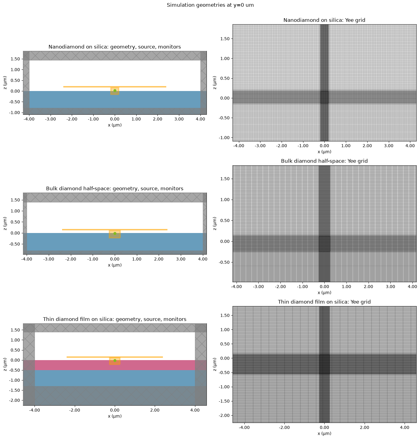
Inspection of the Simulation Domain for All Geometries
The cell below constructs the actual simulation objects for nanodiamond, bulk_halfspace, and diamond_film, and compares the structures, source, monitors, and computational grid in the $y=0$ cross-sectional plane.
Only local simulation objects are generated in this step; no cloud tasks are submitted.
def plot_geometry_gallery(
    configs: Mapping[str, ModelConfig],
    *,
    slice_axis: Literal["x", "y"] = "y",
    slice_position_um: float = 0.0,
) -> dict[str, td.Simulation]:
    """Plot structure/monitor placement and grid for each geometry configuration."""
    if slice_axis not in {"x", "y"}:
        raise ValueError("slice_axis must be 'x' or 'y'.")

    simulations = {}
    fig, axes = plt.subplots(
        len(configs), 2, figsize=(14, 4.8 * len(configs)), squeeze=False
    )
    slice_kwargs = {slice_axis: slice_position_um}

    for row, (label, cfg) in enumerate(configs.items()):
        pair, info = build_nv_transition_pair(cfg)
        sim = pair["t1"]
        sim.validate_pre_upload()
        simulations[label] = sim

        sim.plot(ax=axes[row, 0], **slice_kwargs)
        axes[row, 0].set_title(f"{label}: geometry, source, monitors")
        sim.plot_grid(ax=axes[row, 1], **slice_kwargs)
        axes[row, 1].set_title(f"{label}: Yee grid")

        geom = info["geometry"]
        if cfg.geometry == "nanodiamond":
            geometry_detail = f"diameter={cfg.nd_diameter_nm:g} nm"
        elif cfg.geometry == "bulk_halfspace":
            geometry_detail = f"NV depth={cfg.nv_depth_nm:g} nm"
        else:
            geometry_detail = (
                f"film thickness={cfg.film_thickness_nm:g} nm, "
                f"NV depth={cfg.nv_depth_nm:g} nm"
            )
        print(
            f"{label} ({cfg.geometry}; {geometry_detail}): "
            f"center={sim.center} um, size={sim.size} um, "
            f"NV={geom['nv_position']} um, z=[{geom['z_min']:.3f}, {geom['z_max']:.3f}] um"
        )

    fig.suptitle(
        f"Simulation geometries at {slice_axis}={slice_position_um:g} um", y=1.002
    )
    plt.tight_layout()
    plt.show()
    return simulations


geometry_preview_configs = {
    "Nanodiamond on silica": replace(base_cfg, geometry="nanodiamond"),
    "Bulk diamond half-space": replace(
        base_cfg, geometry="bulk_halfspace", nv_depth_nm=20.0
    ),
    "Thin diamond film on silica": replace(
        base_cfg, geometry="diamond_film", film_thickness_nm=500.0, nv_depth_nm=20.0
    ),
}
geometry_preview_simulations = plot_geometry_gallery(geometry_preview_configs)
Nanodiamond on silica (nanodiamond; diameter=40 nm): center=(0.0, 0.0, 0.31999999999999995) um, size=(8.0, 8.0, 2.24) um, NV=(0.0, 0.0, 0.02) um, z=[-0.800, 1.440] um
Bulk diamond half-space (bulk_halfspace; NV depth=20 nm): center=(0.0, 0.0, 0.29999999999999993) um, size=(8.0, 8.0, 2.2) um, NV=(0.0, 0.0, -0.02) um, z=[-0.800, 1.400] um
Thin diamond film on silica (diamond_film; film thickness=500 nm, NV depth=20 nm): center=(0.0, 0.0, 0.04999999999999993) um, size=(8.0, 8.0, 2.7) um, NV=(0.0, 0.0, -0.02) um, z=[-1.300, 1.400] um
Batch Construction and Cost Estimate
A single NV orientation requires at least two separate simulations because the two optical transition dipoles must be evaluated independently.
Since the number of simulation tasks can increase rapidly during parameter sweeps, the simulations are grouped into a Batch. The helper below prints the maximum estimated computational cost and then submits the batch; it does not pause for confirmation.
def prepare_batch(
    cases: Mapping[str, ModelConfig],
    folder_name: str,
) -> tuple[web.Batch, dict[str, td.Simulation]]:
    simulations: dict[str, td.Simulation] = {}
    for case_name, cfg in cases.items():
        pair, _ = build_nv_transition_pair(cfg)
        simulations[f"{case_name}__t1"] = pair["t1"]
        simulations[f"{case_name}__t2"] = pair["t2"]
    batch = web.Batch(simulations=simulations, folder_name=folder_name, verbose=True)
    return batch, simulations


def run_batch_with_cost_estimate(
    batch: web.Batch,
    path_dir: Path,
    cases: Mapping[str, ModelConfig] | None = None,
):
    path_dir.mkdir(parents=True, exist_ok=True)
    if cases is not None:
        case_definitions = json.loads(
            json.dumps({name: asdict(cfg) for name, cfg in cases.items()})
        )
        manifest_path = path_dir / "case_definitions.json"
        if manifest_path.exists():
            previous_definitions = json.loads(manifest_path.read_text(encoding="utf-8"))
            if previous_definitions != case_definitions:
                raise RuntimeError(
                    f"{manifest_path} describes different simulations. "
                    "Change RESULT_SET_TAG or choose a new result directory before submitting."
                )
        manifest_path.write_text(
            json.dumps(case_definitions, indent=2, sort_keys=True),
            encoding="utf-8",
        )
    estimated_cost = batch.estimate_cost(verbose=True)
    print("Estimated maximum batch cost:", estimated_cost)
    return batch.run(path_dir=path_dir)
7. Baseline Simulation and Post-Processing
Before performing any parameter sweep, run a single baseline case first.
Proceed to the convergence tests in Stage 8 only after confirming that the baseline simulation is physically and numerically well behaved.
single_cases = {"nd40_beta54p7_700nm": base_cfg}
single_batch, single_simulations = prepare_batch(
    single_cases,
    folder_name="NV_collection_single_case",
)

print("Number of simulations:", len(single_simulations))
for task_name, sim in single_simulations.items():
    print(task_name, "cells =", sim.num_cells)

single_data = run_batch_with_cost_estimate(
    single_batch,
    result_dir("stage7_single_case"),
    single_cases,
)
Number of simulations: 2
nd40_beta54p7_700nm__t1 cells = 27342000
nd40_beta54p7_700nm__t2 cells = 27342000
21:23:24 KST Maximum FlexCredit cost: 0.680 for the whole batch.
Output()
Estimated maximum batch cost: 0.679631294311451
21:23:25 KST Started working on Batch containing 2 tasks.
21:23:28 KST Maximum FlexCredit cost: 0.680 for the whole batch.
             Use 'Batch.real_cost()' to get the billed FlexCredit cost after
             completion.
Output()
21:23:29 KST Batch complete.
7.1 Far-Field Cone Integration
The radial Poynting flux of the Tidy3D projected field is given by
$$ S_r = \frac{1}{2} \operatorname{Re} \left( E_\theta H_\phi^* - E_\phi H_\theta^* \right). $$
For a projection radius $r$, the optical power contained within the collection cone is
$$ P_{\mathrm{cone}} = r^2 \int\!\!\int S_r \sin\theta \, d\theta \, d\phi. $$
Tidy3D's built-in integrator requires full-sphere integration over the entire spherical domain, $0 \leq \theta \leq \pi$. Since the present calculation uses only the air-side open projection plane and the objective acceptance cone, the angular integration is implemented numerically.
# NumPy >= 2.0 provides trapezoid; older releases use trapz.
# Use an explicit branch because getattr(..., np.trapz) evaluates np.trapz eagerly.
if hasattr(np, "trapezoid"):
    _TRAPEZOID = np.trapezoid
else:
    _TRAPEZOID = np.trapz


def integrate_angular_power_array(
    power_values: np.ndarray,
    theta: np.ndarray,
    phi: np.ndarray,
    theta_limit_rad: float,
    *,
    projection_radius_um: float = 1.0,
) -> np.ndarray:
    """Integrate S_r over a cone for arrays shaped (theta, phi, ...)."""
    theta = np.asarray(theta, dtype=float)
    phi = np.asarray(phi, dtype=float)
    values = np.real(np.asarray(power_values))

    if values.shape[0] != theta.size or values.shape[1] != phi.size:
        raise ValueError("power_values must have leading dimensions (theta, phi).")

    mask = theta <= theta_limit_rad + 1e-12
    if mask.sum() < 2:
        raise ValueError("Not enough theta samples inside the requested cone.")
    if theta[mask][-1] < theta_limit_rad - 1e-9:
        raise ValueError("theta_limit is not included in the angular grid.")
    if not np.isclose(phi[0], 0.0) or not np.isclose(phi[-1], 2.0 * np.pi):
        raise ValueError("phi must cover 0 to 2pi, including both endpoints.")

    theta_sel = theta[mask]
    values_sel = values[mask, ...]
    sin_shape = (theta_sel.size,) + (1,) * (values_sel.ndim - 1)
    integrand = values_sel * np.sin(theta_sel).reshape(sin_shape)

    integral_phi = _TRAPEZOID(integrand, x=phi, axis=1)
    integral_theta_phi = _TRAPEZOID(integral_phi, x=theta_sel, axis=0)
    return projection_radius_um**2 * integral_theta_phi


def integrate_projected_power_cone(far_data, theta_limit_rad: float) -> np.ndarray:
    """Integrate r^2 S_r over 0 <= theta <= theta_limit and 0 <= phi <= 2pi."""
    power = far_data.power
    if "r" in power.dims:
        power = power.isel(r=0)
    power = power.transpose("theta", "phi", "f")

    theta = np.asarray(power.coords["theta"].values, dtype=float)
    phi = np.asarray(power.coords["phi"].values, dtype=float)
    r_um = float(far_data.monitor.proj_distance)
    return integrate_angular_power_array(
        power.values,
        theta,
        phi,
        theta_limit_rad,
        projection_radius_um=r_um,
    )


# Local unit test: homogeneous-medium z-dipole pattern dP/dOmega proportional to sin^2(theta).
theta_limit_test = theta_objective_rad
theta_test = np.unique(
    np.sort(np.append(np.linspace(0.0, np.pi, 1001), theta_limit_test))
)
phi_test = np.linspace(0.0, 2.0 * np.pi, 721)
dipole_z_pattern = np.sin(theta_test)[:, None] ** 2 * np.ones((1, phi_test.size))
cone_numeric = float(
    integrate_angular_power_array(
        dipole_z_pattern,
        theta_test,
        phi_test,
        theta_limit_test,
    )
)
cos_limit = np.cos(theta_limit_test)
cone_exact = 2.0 * np.pi * (2.0 / 3.0 - cos_limit + cos_limit**3 / 3.0)
assert np.isclose(cone_numeric, cone_exact, rtol=5e-5)
print("Angular-cone integrator unit test passed.")


def _real_1d(data_array) -> np.ndarray:
    return np.real(np.asarray(data_array.values)).reshape(-1)


def extract_transition_metrics(sim_data, cfg: ModelConfig) -> pd.DataFrame:
    total_flux_da = sim_data["total_flux"].flux
    air_flux_da = sim_data["air_flux"].flux
    far_data = sim_data["far_field"]

    freqs = np.asarray(total_flux_da.coords["f"].values, dtype=float)
    p_total = _real_1d(total_flux_da)
    p_air_plane = _real_1d(air_flux_da)

    theta_obj = np.arcsin(cfg.objective_na / cfg.collection_index)
    theta_ff_max = np.deg2rad(cfg.far_theta_max_deg)
    p_na = integrate_projected_power_cone(far_data, theta_obj)
    p_far_cap = integrate_projected_power_cone(far_data, theta_ff_max)

    df = pd.DataFrame(
        {
            "frequency_hz": freqs,
            "wavelength_nm": 1e3 * td.C_0 / freqs,
            "p_total": p_total,
            "p_na": p_na,
            "p_air_plane": p_air_plane,
            "p_far_cap": p_far_cap,
        }
    )
    df["eta_na"] = df["p_na"] / df["p_total"]
    df["eta_air_plane"] = df["p_air_plane"] / df["p_total"]
    df["na_fraction_of_air_plane"] = df["p_na"] / df["p_air_plane"]
    return df.sort_values("wavelength_nm").reset_index(drop=True)


def combine_nv_transitions(t1: pd.DataFrame, t2: pd.DataFrame) -> pd.DataFrame:
    merged = t1.merge(t2, on=["frequency_hz", "wavelength_nm"], suffixes=("_t1", "_t2"))

    out = merged[["frequency_hz", "wavelength_nm"]].copy()
    for quantity in ["p_total", "p_na", "p_air_plane", "p_far_cap"]:
        out[quantity] = merged[f"{quantity}_t1"] + merged[f"{quantity}_t2"]

    out["eta_collection"] = out["p_na"] / out["p_total"]
    out["eta_air_plane"] = out["p_air_plane"] / out["p_total"]
    out["na_fraction_of_air_plane"] = out["p_na"] / out["p_air_plane"]
    out["eta_t1"] = merged["eta_na_t1"]
    out["eta_t2"] = merged["eta_na_t2"]
    return out.sort_values("wavelength_nm").reset_index(drop=True)


def process_case(batch_data, case_name: str, cfg: ModelConfig) -> pd.DataFrame:
    t1_task_name = f"{case_name}__t1"
    t2_task_name = f"{case_name}__t2"
    t1_data = batch_data.load_sim_data(t1_task_name)
    t2_data = batch_data.load_sim_data(t2_task_name)
    for task_name, sim_data in ((t1_task_name, t1_data), (t2_task_name, t2_data)):
        if bool(getattr(sim_data, "diverged", False)):
            raise RuntimeError(
                f"{task_name} diverged; its monitor data cannot be used for efficiency calculations."
            )
    t1 = extract_transition_metrics(t1_data, cfg)
    t2 = extract_transition_metrics(t2_data, cfg)
    result = combine_nv_transitions(t1, t2)

    result.insert(0, "case", case_name)
    result["geometry"] = cfg.geometry
    result["nd_diameter_nm"] = cfg.nd_diameter_nm
    result["nv_depth_nm"] = cfg.nv_depth_nm
    result["film_thickness_nm"] = cfg.film_thickness_nm
    result["nv_beta_deg"] = cfg.nv_beta_deg
    result["nv_alpha_deg"] = cfg.nv_alpha_deg
    result["mesh_dl_nm"] = cfg.mesh_dl_nm
    result["xy_span_um"] = cfg.xy_span_um
    result["projection_span_um"] = cfg.projection_span_um
    result["air_buffer_um"] = cfg.air_buffer_um
    result["substrate_buffer_um"] = cfg.substrate_buffer_um
    result["boundary_scheme"] = (
        f"xy_absorber{cfg.film_absorber_num_layers}_zminus_absorber_zplus_pml"
        if cfg.geometry == "diamond_film"
        else "all_pml"
    )
    result["lateral_monitor_to_pml_um"] = 0.5 * (
        cfg.xy_span_um - cfg.projection_span_um
    )
    result["vertical_monitor_to_pml_um"] = cfg.air_buffer_um - cfg.projection_gap_um
    longest_wavelength_um = 1e-3 * max(cfg.wavelengths_nm)
    result["lateral_clearance_wavelengths"] = (
        result["lateral_monitor_to_pml_um"] / longest_wavelength_um
    )
    result["vertical_clearance_wavelengths"] = (
        result["vertical_monitor_to_pml_um"] / longest_wavelength_um
    )
    result["diamond_model"] = cfg.diamond_model
    result["nv_offset_x_nm"] = cfg.nv_offset_nm[0]
    result["nv_offset_y_nm"] = cfg.nv_offset_nm[1]
    result["nv_offset_z_nm"] = cfg.nv_offset_nm[2]
    if cfg.geometry == "nanodiamond":
        result["nd_top_surface_depth_nm"] = (
            0.5 * cfg.nd_diameter_nm - cfg.nv_offset_nm[2]
        )
        result["nv_height_above_substrate_nm"] = (
            0.5 * cfg.nd_diameter_nm - cfg.nd_embed_nm + cfg.nv_offset_nm[2]
        )
    else:
        result["nd_top_surface_depth_nm"] = np.nan
        result["nv_height_above_substrate_nm"] = np.nan
    return result


def collect_batch_results(batch_data, cases: Mapping[str, ModelConfig]) -> pd.DataFrame:
    frames = [
        process_case(batch_data, case_name, cfg) for case_name, cfg in cases.items()
    ]
    return pd.concat(frames, ignore_index=True)
Angular-cone integrator unit test passed.
if single_data is not None:
    single_df = collect_batch_results(single_data, single_cases)
    display(single_df)

    ax = single_df.plot(
        x="wavelength_nm",
        y=["eta_collection", "eta_air_plane"],
        marker="o",
        figsize=(7, 4),
    )
    ax.set_ylabel("Efficiency")
    ax.grid(True)
    plt.show()
else:
    print(
        "No baseline BatchData is available. Run the Stage 7 batch cell before post-processing."
    )
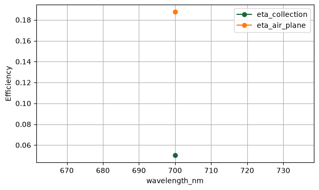
| case | frequency_hz | wavelength_nm | p_total | p_na | p_air_plane | p_far_cap | eta_collection | eta_air_plane | na_fraction_of_air_plane | ... | lateral_monitor_to_pml_um | vertical_monitor_to_pml_um | lateral_clearance_wavelengths | vertical_clearance_wavelengths | diamond_model | nv_offset_x_nm | nv_offset_y_nm | nv_offset_z_nm | nd_top_surface_depth_nm | nv_height_above_substrate_nm | |
|---|---|---|---|---|---|---|---|---|---|---|---|---|---|---|---|---|---|---|---|---|---|
| 0 | nd40_beta54p7_700nm | 4.282749e+14 | 700.0 | 1.516450e-27 | 7.595780e-29 | 2.843069e-28 | 2.675983e-28 | 0.050089 | 0.187482 | 0.267168 | ... | 1.6 | 1.25 | 2.285714 | 1.785714 | peter_sellmeier | 0.0 | 0.0 | 0.0 | 20.0 | 20.0 |
1 rows × 34 columns
8. Numerical Convergence Tests
Before performing the final physical parameter sweeps, at least the following two convergence tests should be carried out.
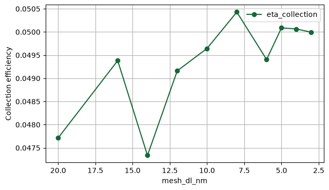
8.1 Local Mesh Convergence
The sweep below samples ten local mesh spacings from 20 nm down to 3 nm. The coarsest values intentionally under-resolve a 40 nm nanodiamond and serve only to reveal the convergence trend; final results should be taken from the converged fine-mesh region.
An example definition of the relative convergence error is
$$ \epsilon_i = \frac{ \left|\eta_i-\eta_{\mathrm{finest}}\right| }{ \eta_{\mathrm{finest}} }. $$
8.2 Projection-Plane Span Convergence
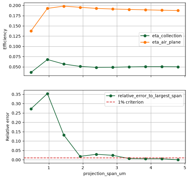
For an open near-to-far-field projection surface, the field amplitude should be sufficiently small near the edges of the projection plane.
The parameter projection_span_um is therefore increased systematically to verify that $\eta_{\mathrm{coll}}$ converges to a stable value. To isolate aperture truncation from domain/PML effects, xy_span_um is held fixed at 8.0 µm for every case in this sweep. The largest 4.8 µm projection plane retains 1.6 µm of non-PML clearance on each lateral side, corresponding to about 2.3 vacuum wavelengths at 700 nm.
Caution: Convergence with respect to the projection-plane span should not be verified only once for the baseline nanodiamond case. The test should also be repeated for representative conditions in which the angular spectrum may differ significantly, such as the bulk-diamond and diamond-film geometries, the shortest wavelength, and the largest nanodiamond.
CONVERGENCE_RTOL = 0.01
mesh_values_nm = [20.0, 16.0, 14.0, 12.0, 10.0, 8.0, 6.0, 5.0, 4.0, 3.0]
mesh_cases = {
    f"mesh_{str(dl).replace('.', 'p')}nm": replace(base_cfg, mesh_dl_nm=dl)
    for dl in mesh_values_nm
}

projection_spans_um = [0.48, 0.96, 1.44, 1.92, 2.40, 2.88, 3.36, 3.84, 4.32, 4.8]
SPAN_SWEEP_FIXED_DOMAIN_UM = LARGE_DOMAIN_XY_SPAN_UM
span_cases = {
    f"span_{str(span).replace('.', 'p')}um": replace(
        base_cfg,
        projection_span_um=span,
        xy_span_um=SPAN_SWEEP_FIXED_DOMAIN_UM,
    )
    for span in projection_spans_um
}

print("Mesh convergence cases:", list(mesh_cases))
print("Projection-span convergence cases:", list(span_cases))
Mesh convergence cases: ['mesh_20p0nm', 'mesh_16p0nm', 'mesh_14p0nm', 'mesh_12p0nm', 'mesh_10p0nm', 'mesh_8p0nm', 'mesh_6p0nm', 'mesh_5p0nm', 'mesh_4p0nm', 'mesh_3p0nm']
Projection-span convergence cases: ['span_0p48um', 'span_0p96um', 'span_1p44um', 'span_1p92um', 'span_2p4um', 'span_2p88um', 'span_3p36um', 'span_3p84um', 'span_4p32um', 'span_4p8um']
mesh_batch, _ = prepare_batch(mesh_cases, folder_name="NV_collection_mesh_convergence")
mesh_data = run_batch_with_cost_estimate(
    mesh_batch, result_dir("stage8_mesh_convergence"), mesh_cases
)
21:24:46 KST Maximum FlexCredit cost: 5.141 for the whole batch.
Output()
Estimated maximum batch cost: 5.1412896046428695
21:24:48 KST Started working on Batch containing 20 tasks.
21:25:11 KST Maximum FlexCredit cost: 5.141 for the whole batch.
             Use 'Batch.real_cost()' to get the billed FlexCredit cost after
             completion.
Output()
21:25:26 KST Batch complete.
span_batch, _ = prepare_batch(span_cases, folder_name="NV_collection_span_convergence")
span_data = run_batch_with_cost_estimate(
    span_batch, result_dir("stage8_span_convergence"), span_cases
)
21:26:39 KST Maximum FlexCredit cost: 6.791 for the whole batch.
Output()
Estimated maximum batch cost: 6.791108951113984
21:26:40 KST Started working on Batch containing 20 tasks.
21:27:04 KST Maximum FlexCredit cost: 6.791 for the whole batch.
             Use 'Batch.real_cost()' to get the billed FlexCredit cost after
             completion.
Output()
21:27:19 KST Batch complete.
mesh_data = globals().get("mesh_data")
span_data = globals().get("span_data")

if mesh_data is not None:
    mesh_df = collect_batch_results(mesh_data, mesh_cases)
    mesh_one = mesh_df.loc[mesh_df.groupby("case")["wavelength_nm"].idxmin()].copy()
    mesh_one = mesh_one.sort_values("mesh_dl_nm", ascending=False)
    eta_ref = mesh_one.sort_values("mesh_dl_nm").iloc[0]["eta_collection"]
    mesh_one["relative_error_to_finest"] = np.abs(
        mesh_one["eta_collection"] - eta_ref
    ) / abs(eta_ref)
    display(mesh_one[["mesh_dl_nm", "eta_collection", "relative_error_to_finest"]])

    ax = mesh_one.plot(x="mesh_dl_nm", y="eta_collection", marker="o", figsize=(7, 4))
    ax.invert_xaxis()
    ax.set_ylabel("Collection efficiency")
    ax.grid(True)
    plt.show()

if span_data is not None:
    span_df = collect_batch_results(span_data, span_cases)
    span_one = span_df.loc[span_df.groupby("case")["wavelength_nm"].idxmin()].copy()
    span_one = span_one.sort_values("projection_span_um")
    eta_ref = span_one.iloc[-1]["eta_collection"]
    span_one["relative_error_to_largest_span"] = np.abs(
        span_one["eta_collection"] - eta_ref
    ) / abs(eta_ref)
    span_one["relative_change_from_previous"] = (
        span_one["eta_collection"].pct_change().abs()
    )
    span_one["converged_to_largest_span"] = (
        span_one["relative_error_to_largest_span"] <= CONVERGENCE_RTOL
    )
    span_columns = [
        "projection_span_um",
        "xy_span_um",
        "eta_collection",
        "lateral_monitor_to_pml_um",
        "lateral_clearance_wavelengths",
        "p_total",
        "p_na",
        "p_air_plane",
        "eta_air_plane",
        "na_fraction_of_air_plane",
        "relative_change_from_previous",
        "relative_error_to_largest_span",
        "converged_to_largest_span",
    ]
    display(span_one[span_columns])
    final_step_change = float(span_one.iloc[-1]["relative_change_from_previous"])
    if final_step_change > CONVERGENCE_RTOL:
        print(
            f"WARNING: the two largest projection spans differ by {final_step_change:.2%}; "
            "the aperture sweep has not met the 1% consecutive-step criterion."
        )
    else:
        print(
            f"Largest-span consecutive change: {final_step_change:.2%}. "
            "Confirm this plateau with the independent domain/PML sweeps in Stage 8B."
        )

    fig, axes = plt.subplots(2, 1, figsize=(7, 7), sharex=True)
    span_one.plot(
        x="projection_span_um",
        y=["eta_collection", "eta_air_plane"],
        marker="o",
        ax=axes[0],
    )
    axes[0].set_ylabel("Efficiency")
    axes[0].grid(True)
    span_one.plot(
        x="projection_span_um",
        y="relative_error_to_largest_span",
        marker="o",
        ax=axes[1],
        legend=False,
    )
    axes[1].axhline(
        CONVERGENCE_RTOL, color="tab:red", linestyle="--", label="1% criterion"
    )
    axes[1].set_ylabel("Relative error")
    axes[1].grid(True)
    axes[1].legend()
    plt.show()
| mesh_dl_nm | eta_collection | relative_error_to_finest | |
|---|---|---|---|
| 0 | 20.0 | 0.047714 | 0.045617 |
| 1 | 16.0 | 0.049382 | 0.012258 |
| 2 | 14.0 | 0.047336 | 0.053170 |
| 3 | 12.0 | 0.049162 | 0.016647 |
| 4 | 10.0 | 0.049645 | 0.006999 |
| 5 | 8.0 | 0.050430 | 0.008715 |
| 6 | 6.0 | 0.049406 | 0.011773 |
| 7 | 5.0 | 0.050089 | 0.001895 |
| 8 | 4.0 | 0.050065 | 0.001405 |
| 9 | 3.0 | 0.049995 | 0.000000 |
| projection_span_um | xy_span_um | eta_collection | lateral_monitor_to_pml_um | lateral_clearance_wavelengths | p_total | p_na | p_air_plane | eta_air_plane | na_fraction_of_air_plane | relative_change_from_previous | relative_error_to_largest_span | converged_to_largest_span | |
|---|---|---|---|---|---|---|---|---|---|---|---|---|---|
| 0 | 0.48 | 8.0 | 0.036422 | 3.76 | 5.371429 | 1.516450e-27 | 5.523265e-29 | 2.090975e-28 | 0.137886 | 0.264148 | NaN | 0.272851 | False |
| 1 | 0.96 | 8.0 | 0.067806 | 3.52 | 5.028571 | 1.516450e-27 | 1.028241e-28 | 2.922718e-28 | 0.192734 | 0.351810 | 0.861654 | 0.353700 | False |
| 2 | 1.44 | 8.0 | 0.056733 | 3.28 | 4.685714 | 1.516450e-27 | 8.603213e-29 | 3.006119e-28 | 0.198234 | 0.286190 | 0.163308 | 0.132631 | False |
| 3 | 1.92 | 8.0 | 0.051002 | 3.04 | 4.342857 | 1.516450e-27 | 7.734229e-29 | 2.962144e-28 | 0.195334 | 0.261102 | 0.101007 | 0.018227 | False |
| 4 | 2.40 | 8.0 | 0.048615 | 2.80 | 4.000000 | 1.516450e-27 | 7.372293e-29 | 2.922630e-28 | 0.192728 | 0.252249 | 0.046797 | 0.029423 | False |
| 5 | 2.88 | 8.0 | 0.048894 | 2.56 | 3.657143 | 1.516450e-27 | 7.414571e-29 | 2.899769e-28 | 0.191221 | 0.255695 | 0.005735 | 0.023857 | False |
| 6 | 3.36 | 8.0 | 0.049766 | 2.32 | 3.314286 | 1.516450e-27 | 7.546727e-29 | 2.884043e-28 | 0.190184 | 0.261672 | 0.017824 | 0.006458 | True |
| 7 | 3.84 | 8.0 | 0.050361 | 2.08 | 2.971429 | 1.516450e-27 | 7.636956e-29 | 2.869337e-28 | 0.189214 | 0.266158 | 0.011956 | 0.005421 | True |
| 8 | 4.32 | 8.0 | 0.050365 | 1.84 | 2.628571 | 1.516450e-27 | 7.637595e-29 | 2.855175e-28 | 0.188280 | 0.267500 | 0.000084 | 0.005505 | True |
| 9 | 4.80 | 8.0 | 0.050089 | 1.60 | 2.285714 | 1.516450e-27 | 7.595780e-29 | 2.843069e-28 | 0.187482 | 0.267168 | 0.005475 | 0.000000 | True |
Largest-span consecutive change: 0.55%. Confirm this plateau with the independent domain/PML sweeps in Stage 8B.
8B. Independent Lateral- and Vertical-PML Convergence Tests
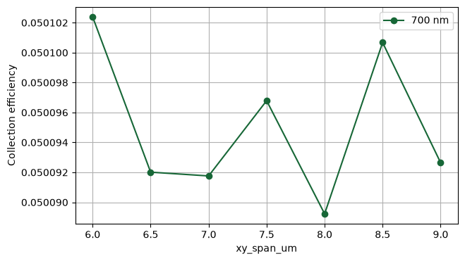
The projection-aperture convergence test is already performed in Stage 8.2 with a fixed 8.0 µm lateral domain. This stage independently tests the lateral and vertical distances to the PML.
For the lateral domain/PML test, projection_span_um is held fixed at 4.8 µm while xy_span_um is varied from 6.0 to 9.0 µm. This includes direct comparisons at 6, 7, 8, and 9 µm.
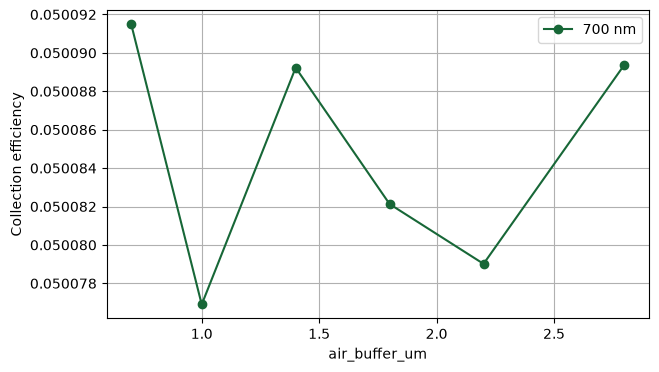
For the vertical PML test, xy_span_um=8.0 µm and projection_span_um=4.8 µm are fixed while air_buffer_um is varied from 0.7 to 2.8 µm. Since the projection plane is projection_gap_um=0.15 µm above the object, its distance to the +z PML start is air_buffer_um - projection_gap_um.
The 0.7 µm air-buffer case is retained only as an intentionally close diagnostic point. The baseline uses 1.4 µm. A half-wavelength clearance is treated only as a construction guard; numerical convergence, rather than that guard, determines the final accepted distance.
For each sweep, the eta_collection value obtained from the largest tested case is used as the reference. The relative error and the corresponding convergence pass/fail criterion are then evaluated with respect to this reference value.
DOMAIN_SWEEP_FIXED_PROJECTION_UM = LARGE_PROJECTION_SPAN_UM
# With a fixed 3.2 um projection plane, the monitor-to-PML-start clearance
# increases from 0.90 um to 2.65 um across this sweep.
domain_xy_spans_um = [6.0, 6.5, 7.0, 7.5, 8.0, 8.5, 9.0]
domain_cases = {
    f"domain_{str(xy).replace('.', 'p')}um": replace(
        base_cfg,
        xy_span_um=xy,
        projection_span_um=DOMAIN_SWEEP_FIXED_PROJECTION_UM,
    )
    for xy in domain_xy_spans_um
}

air_buffer_values_um = [0.70, 1.00, 1.40, 1.80, 2.20, 2.80]
air_buffer_cases = {
    f"air_buffer_{str(buffer).replace('.', 'p')}um": replace(
        base_cfg,
        air_buffer_um=buffer,
        xy_span_um=LARGE_DOMAIN_XY_SPAN_UM,
        projection_span_um=LARGE_PROJECTION_SPAN_UM,
    )
    for buffer in air_buffer_values_um
}
print("Domain/PML cases:", list(domain_cases))
print("Air-buffer/PML cases:", list(air_buffer_cases))
print("Total FDTD simulations:", 2 * (len(domain_cases) + len(air_buffer_cases)))
Domain/PML cases: ['domain_6p0um', 'domain_6p5um', 'domain_7p0um', 'domain_7p5um', 'domain_8p0um', 'domain_8p5um', 'domain_9p0um']
Air-buffer/PML cases: ['air_buffer_0p7um', 'air_buffer_1p0um', 'air_buffer_1p4um', 'air_buffer_1p8um', 'air_buffer_2p2um', 'air_buffer_2p8um']
Total FDTD simulations: 26
domain_batch, _ = prepare_batch(
    domain_cases, folder_name="NV_collection_domain_pml_convergence"
)
domain_data = run_batch_with_cost_estimate(
    domain_batch, result_dir("stage8b_domain_pml_convergence"), domain_cases
)
21:28:12 KST Maximum FlexCredit cost: 4.346 for the whole batch.
Output()
Estimated maximum batch cost: 4.34630537629622
21:28:13 KST Started working on Batch containing 14 tasks.
WARNING: No connection: Retrying for 180 seconds.
21:28:32 KST Maximum FlexCredit cost: 4.346 for the whole batch.
             Use 'Batch.real_cost()' to get the billed FlexCredit cost after
             completion.
Output()
21:28:43 KST Batch complete.
air_buffer_batch, _ = prepare_batch(
    air_buffer_cases, folder_name="NV_collection_air_buffer_pml_convergence"
)
air_buffer_data = run_batch_with_cost_estimate(
    air_buffer_batch, result_dir("stage8b_air_buffer_pml_convergence"), air_buffer_cases
)
21:29:27 KST Maximum FlexCredit cost: 4.186 for the whole batch.
Output()
Estimated maximum batch cost: 4.186049905271815
21:29:28 KST Started working on Batch containing 12 tasks.
21:29:43 KST Maximum FlexCredit cost: 4.186 for the whole batch.
             Use 'Batch.real_cost()' to get the billed FlexCredit cost after
             completion.
Output()
21:29:53 KST Batch complete.
def convergence_against_largest_case(
    result_df: pd.DataFrame, x_col: str, rtol: float = CONVERGENCE_RTOL
) -> pd.DataFrame:
    """Compare eta_collection at each wavelength with the largest-x case."""
    largest_x = float(result_df[x_col].max())
    reference = result_df.loc[
        np.isclose(result_df[x_col], largest_x), ["wavelength_nm", "eta_collection"]
    ].rename(columns={"eta_collection": "eta_reference"})
    out = result_df.merge(
        reference, on="wavelength_nm", how="left", validate="many_to_one"
    )
    denominator = np.maximum(np.abs(out["eta_reference"]), np.finfo(float).eps)
    out["relative_error_to_largest"] = (
        np.abs(out["eta_collection"] - out["eta_reference"]) / denominator
    )
    numerical_slack = 10.0 * np.finfo(float).eps
    out["converged"] = out["relative_error_to_largest"] <= rtol + numerical_slack
    out = out.sort_values(["wavelength_nm", x_col]).reset_index(drop=True)
    out["relative_change_from_previous"] = (
        out.groupby("wavelength_nm")["eta_collection"].pct_change().abs()
    )
    return out


def report_size_convergence(batch_data, cases, x_col: str, output_csv: Path):
    if batch_data is None:
        print(f"{x_col}: no cloud result loaded.")
        return None
    collected = collect_batch_results(batch_data, cases)
    if x_col not in collected.columns:
        collected[x_col] = collected["case"].map(
            {name: getattr(cfg, x_col) for name, cfg in cases.items()}
        )
    summary = convergence_against_largest_case(collected, x_col)
    output_csv.parent.mkdir(parents=True, exist_ok=True)
    summary.to_csv(output_csv, index=False)
    cols = [
        "wavelength_nm",
        x_col,
        "projection_span_um",
        "eta_collection",
        "lateral_monitor_to_pml_um",
        "vertical_monitor_to_pml_um",
        "lateral_clearance_wavelengths",
        "vertical_clearance_wavelengths",
        "eta_air_plane",
        "relative_change_from_previous",
        "eta_reference",
        "relative_error_to_largest",
        "converged",
    ]
    display(summary[cols])
    _fig, ax = plt.subplots(figsize=(7, 4))
    for wavelength_nm, group in summary.groupby("wavelength_nm"):
        group = group.sort_values(x_col)
        ax.plot(
            group[x_col],
            group["eta_collection"],
            marker="o",
            label=f"{wavelength_nm:g} nm",
        )
    ax.set(xlabel=x_col, ylabel="Collection efficiency")
    ax.grid(True)
    ax.legend()
    plt.show()
    return summary


domain_convergence_df = report_size_convergence(
    globals().get("domain_data"),
    domain_cases,
    "xy_span_um",
    result_dir("stage8b_domain_pml_convergence") / "domain_convergence.csv",
)
air_buffer_convergence_df = report_size_convergence(
    globals().get("air_buffer_data"),
    air_buffer_cases,
    "air_buffer_um",
    result_dir("stage8b_air_buffer_pml_convergence") / "air_buffer_convergence.csv",
)
| wavelength_nm | xy_span_um | projection_span_um | eta_collection | lateral_monitor_to_pml_um | vertical_monitor_to_pml_um | lateral_clearance_wavelengths | vertical_clearance_wavelengths | eta_air_plane | relative_change_from_previous | eta_reference | relative_error_to_largest | converged | |
|---|---|---|---|---|---|---|---|---|---|---|---|---|---|
| 0 | 700.0 | 6.0 | 4.8 | 0.050102 | 0.60 | 1.25 | 0.857143 | 1.785714 | 0.187543 | NaN | 0.050093 | 0.000195 | True |
| 1 | 700.0 | 6.5 | 4.8 | 0.050092 | 0.85 | 1.25 | 1.214286 | 1.785714 | 0.187494 | 0.000207 | 0.050093 | 0.000013 | True |
| 2 | 700.0 | 7.0 | 4.8 | 0.050092 | 1.10 | 1.25 | 1.571429 | 1.785714 | 0.187496 | 0.000005 | 0.050093 | 0.000018 | True |
| 3 | 700.0 | 7.5 | 4.8 | 0.050097 | 1.35 | 1.25 | 1.928571 | 1.785714 | 0.187516 | 0.000100 | 0.050093 | 0.000083 | True |
| 4 | 700.0 | 8.0 | 4.8 | 0.050089 | 1.60 | 1.25 | 2.285714 | 1.785714 | 0.187482 | 0.000151 | 0.050093 | 0.000068 | True |
| 5 | 700.0 | 8.5 | 4.8 | 0.050101 | 1.85 | 1.25 | 2.642857 | 1.785714 | 0.187535 | 0.000228 | 0.050093 | 0.000160 | True |
| 6 | 700.0 | 9.0 | 4.8 | 0.050093 | 2.10 | 1.25 | 3.000000 | 1.785714 | 0.187497 | 0.000160 | 0.050093 | 0.000000 | True |
| wavelength_nm | air_buffer_um | projection_span_um | eta_collection | lateral_monitor_to_pml_um | vertical_monitor_to_pml_um | lateral_clearance_wavelengths | vertical_clearance_wavelengths | eta_air_plane | relative_change_from_previous | eta_reference | relative_error_to_largest | converged | |
|---|---|---|---|---|---|---|---|---|---|---|---|---|---|
| 0 | 700.0 | 0.7 | 4.8 | 0.050091 | 1.6 | 0.55 | 2.285714 | 0.785714 | 0.187484 | NaN | 0.050089 | 0.000042 | True |
| 1 | 700.0 | 1.0 | 4.8 | 0.050077 | 1.6 | 0.85 | 2.285714 | 1.214286 | 0.187468 | 0.000291 | 0.050089 | 0.000249 | True |
| 2 | 700.0 | 1.4 | 4.8 | 0.050089 | 1.6 | 1.25 | 2.285714 | 1.785714 | 0.187482 | 0.000246 | 0.050089 | 0.000003 | True |
| 3 | 700.0 | 1.8 | 4.8 | 0.050082 | 1.6 | 1.65 | 2.285714 | 2.357143 | 0.187477 | 0.000142 | 0.050089 | 0.000145 | True |
| 4 | 700.0 | 2.2 | 4.8 | 0.050079 | 1.6 | 2.05 | 2.285714 | 2.928571 | 0.187468 | 0.000062 | 0.050089 | 0.000207 | True |
| 5 | 700.0 | 2.8 | 4.8 | 0.050089 | 1.6 | 2.65 | 2.285714 | 3.785714 | 0.187481 | 0.000207 | 0.050089 | 0.000000 | True |
9. Nanodiamond Diameter Sweep
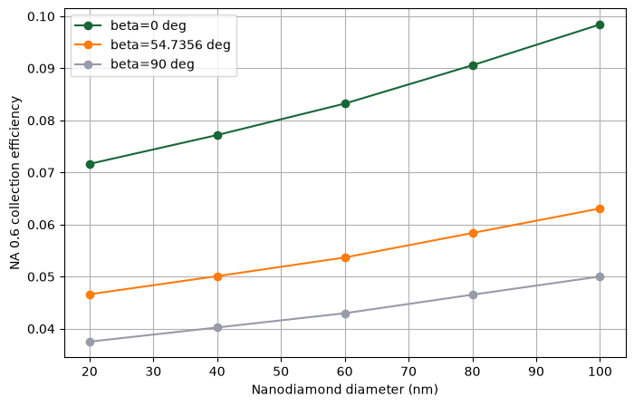
Changing the nanodiamond diameter can simultaneously affect:
- The local density of optical states (LDOS) around the NV center
- Interference associated with the diamond–air and diamond–silica interfaces
- The angular radiation pattern of the dielectric particle
- Resonant effects when the particle size becomes comparable to the wavelength inside the diamond
For a diameter sweep, the definition of the NV position must be specified explicitly.
-
center: The NV center is placed at the center of the nanodiamond for every diameter. In this case, the distance from the NV center to the top surface is $d/2$, so the nanodiamond diameter and the NV surface depth vary simultaneously. -
fixed_top_depth: The NV center is maintained at a fixed depth below the top surface for every nanodiamond diameter. This partially separates the effect of particle geometry from variations in the top-surface depth. However, the distance to the substrate and the distances to the lateral surfaces may still vary with nanodiamond diameter.
The default setting below is center. By changing DIAMETER_POSITION_MODE, the two cases can be calculated and stored in separate directories for direct comparison.
Representative NV-axis polar angles are $0^\circ$, $54.7356^\circ$, and $90^\circ$.
For small nanodiamonds, the local mesh spacing is automatically constrained to a smaller value to ensure a sufficient number of grid cells across the particle diameter.
diameters_nm = [20.0, 40.0, 60.0, 80.0, 100.0]
representative_betas_deg = [0.0, 54.7356, 90.0]

DIAMETER_POSITION_MODE = "center"
FIXED_TOP_DEPTH_NM = 10.0
CONVERGED_MESH_NM = 5.0


def nd_offset_for_top_surface_depth(
    diameter_nm: float,
    top_depth_nm: float,
) -> tuple[float, float, float]:
    """Return sphere-center-referenced NV offset for a specified top-surface depth."""
    if not (0.0 < top_depth_nm < diameter_nm):
        raise ValueError("Require 0 < top_depth_nm < diameter_nm.")
    radius_nm = 0.5 * diameter_nm
    return (0.0, 0.0, radius_nm - top_depth_nm)


if DIAMETER_POSITION_MODE not in {"center", "fixed_top_depth"}:
    raise ValueError("DIAMETER_POSITION_MODE must be 'center' or 'fixed_top_depth'.")


diameter_cases: dict[str, ModelConfig] = {}
for diameter_nm in diameters_nm:
    if DIAMETER_POSITION_MODE == "center":
        nv_offset_nm = (0.0, 0.0, 0.0)
    else:
        nv_offset_nm = nd_offset_for_top_surface_depth(
            diameter_nm,
            FIXED_TOP_DEPTH_NM,
        )

    for beta_deg in representative_betas_deg:
        local_dl_nm = min(CONVERGED_MESH_NM, diameter_nm / 8.0)
        name = f"{DIAMETER_POSITION_MODE}_d{int(diameter_nm)}_b{beta_deg:.1f}".replace(
            ".", "p"
        )
        diameter_cases[name] = replace(
            base_cfg,
            nd_diameter_nm=diameter_nm,
            nv_offset_nm=nv_offset_nm,
            nv_beta_deg=beta_deg,
            mesh_dl_nm=local_dl_nm,
        )


diameter_result_dir = result_dir(f"stage9_diameter_sweep_{DIAMETER_POSITION_MODE}")

print("NV position mode:", DIAMETER_POSITION_MODE)
if DIAMETER_POSITION_MODE == "fixed_top_depth":
    print("Fixed top-surface depth (nm):", FIXED_TOP_DEPTH_NM)
print("Cases:", len(diameter_cases))
print("FDTD simulations including two transitions:", 2 * len(diameter_cases))
NV position mode: center
Cases: 15
FDTD simulations including two transitions: 30
diameter_batch, _ = prepare_batch(
    diameter_cases,
    folder_name=f"NV_collection_diameter_sweep_{DIAMETER_POSITION_MODE}",
)
diameter_data = run_batch_with_cost_estimate(
    diameter_batch,
    diameter_result_dir,
    diameter_cases,
)
21:31:49 KST Maximum FlexCredit cost: 16.096 for the whole batch.
Output()
Estimated maximum batch cost: 16.09558698130048
21:31:51 KST Started working on Batch containing 30 tasks.
21:32:47 KST Maximum FlexCredit cost: 16.096 for the whole batch.
             Use 'Batch.real_cost()' to get the billed FlexCredit cost after
             completion.
Output()
21:33:08 KST Batch complete.
if diameter_data is not None:
    diameter_df = collect_batch_results(diameter_data, diameter_cases)
    diameter_df.to_csv(diameter_result_dir / "diameter_sweep.csv", index=False)

    fig, ax = plt.subplots(figsize=(8, 5))
    for beta_deg, group in diameter_df.groupby("nv_beta_deg"):
        group = group.sort_values("nd_diameter_nm")
        ax.plot(
            group["nd_diameter_nm"],
            group["eta_collection"],
            marker="o",
            label=f"beta={beta_deg:g} deg",
        )
    ax.set_xlabel("Nanodiamond diameter (nm)")
    ax.set_ylabel("NA 0.6 collection efficiency")
    ax.grid(True)
    ax.legend()
    plt.show()
10. NV-Axis Orientation Sweep
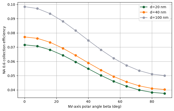
If a spherical nanodiamond is centered on the substrate and the NV center is located exactly at the particle center, the geometry is rotationally symmetric about the $z$ axis. Under this idealized condition, the collection efficiency should, in principle, depend on the polar angle $\beta$ rather than on the azimuthal angle $\alpha$.
Dependence on $\alpha$ should also be evaluated in cases where:
- The NV center is displaced from the center of the nanodiamond
- The nanodiamond is faceted or nonspherical
- The particle is tilted
- Asymmetric structures are present in the surrounding environment
The example below evaluates $\beta$ from $0^\circ$ to $90^\circ$ in increments of $10^\circ$.
orientation_diameters_nm = [20.0, 40.0, 100.0]
beta_values_deg = np.arange(0.0, 90.0 + 1e-9, 8.0)

orientation_cases: dict[str, ModelConfig] = {}
for diameter_nm in orientation_diameters_nm:
    for beta_deg in beta_values_deg:
        name = f"d{int(diameter_nm)}_beta{int(beta_deg)}"
        orientation_cases[name] = replace(
            base_cfg,
            nd_diameter_nm=diameter_nm,
            nv_beta_deg=float(beta_deg),
            mesh_dl_nm=min(CONVERGED_MESH_NM, diameter_nm / 8.0),
        )

print("Cases:", len(orientation_cases))
print("FDTD simulations including two transitions:", 2 * len(orientation_cases))
Cases: 36
FDTD simulations including two transitions: 72
orientation_batch, _ = prepare_batch(
    orientation_cases,
    folder_name="NV_collection_orientation_sweep",
)
orientation_data = run_batch_with_cost_estimate(
    orientation_batch,
    result_dir("stage10_orientation_sweep"),
    orientation_cases,
)
21:37:41 KST Maximum FlexCredit cost: 48.234 for the whole batch.
Output()
Estimated maximum batch cost: 48.23370786531777
21:37:46 KST Started working on Batch containing 72 tasks.
21:39:26 KST Maximum FlexCredit cost: 48.234 for the whole batch.
             Use 'Batch.real_cost()' to get the billed FlexCredit cost after
             completion.
Output()
21:40:22 KST Batch complete.
if orientation_data is not None:
    orientation_df = collect_batch_results(orientation_data, orientation_cases)
    orientation_df.to_csv(
        result_dir("stage10_orientation_sweep") / "orientation_sweep.csv", index=False
    )

    fig, ax = plt.subplots(figsize=(8, 5))
    for diameter_nm, group in orientation_df.groupby("nd_diameter_nm"):
        group = group.sort_values("nv_beta_deg")
        ax.plot(
            group["nv_beta_deg"],
            group["eta_collection"],
            marker="o",
            label=f"d={diameter_nm:g} nm",
        )
    ax.set_xlabel("NV-axis polar angle beta (deg)")
    ax.set_ylabel("NA 0.6 collection efficiency")
    ax.grid(True)
    ax.legend()
    plt.show()
11. Comparison of Nanodiamond, Bulk Half-Space, and Finite Diamond Film
For a fair comparison, two different comparison schemes should be distinguished:
-
Comparison under actual experimental conditions:
Use the actual NV position for each sample geometry. -
Comparison at the same distance from the top surface:
For a 40 nm-diameter nanodiamond with the NV center located at its center, the NV is 20 nm below the top surface. Accordingly, the NV depth in the bulk-diamond and diamond-film geometries is also set to 20 nm.
The code below implements the second comparison scheme.
The diamond-film thickness is set to 500 nm as an example.
Thin-film boundary-stability note
The laterally infinite diamond/silica film stack supports guided modes that propagate into the x/y absorbing boundaries. A standard PML can become numerically unstable when dispersive Sellmeier media extend into it; in test runs, both thin-film transition-dipole simulations diverged, whereas the nanodiamond and bulk cases decayed normally. Therefore,
diamond_filmuses 40-layer adiabatic absorbers on x/y and -z, while the homogeneous-air +z boundary retains a PML. Nanodiamond and bulk cases retain the original all-PML boundary scheme.
comparison_wavelength_nm = 700.0
comparison_beta_deg = 54.7356
matched_surface_distance_nm = 20.0

comparison_cases = {
    "nanodiamond_d40": replace(
        base_cfg,
        geometry="nanodiamond",
        wavelengths_nm=(comparison_wavelength_nm,),
        nd_diameter_nm=40.0,
        nv_offset_nm=(0.0, 0.0, 0.0),
        nv_beta_deg=comparison_beta_deg,
    ),
    "bulk_depth20": replace(
        base_cfg,
        geometry="bulk_halfspace",
        wavelengths_nm=(comparison_wavelength_nm,),
        nv_depth_nm=matched_surface_distance_nm,
        nv_beta_deg=comparison_beta_deg,
    ),
    "film500_depth20": replace(
        base_cfg,
        geometry="diamond_film",
        wavelengths_nm=(comparison_wavelength_nm,),
        film_thickness_nm=500.0,
        nv_depth_nm=matched_surface_distance_nm,
        nv_beta_deg=comparison_beta_deg,
    ),
}

for name, cfg in comparison_cases.items():
    print(
        name, cfg.geometry, "NV depth/diameter =", cfg.nv_depth_nm, cfg.nd_diameter_nm
    )
nanodiamond_d40 nanodiamond NV depth/diameter = 20.0 40.0
bulk_depth20 bulk_halfspace NV depth/diameter = 20.0 40.0
film500_depth20 diamond_film NV depth/diameter = 20.0 40.0
comparison_batch, _ = prepare_batch(
    comparison_cases,
    folder_name="NV_collection_geometry_comparison",
)
comparison_data = run_batch_with_cost_estimate(
    comparison_batch,
    result_dir("stage11_geometry_comparison"),
    comparison_cases,
)
21:40:46 KST Maximum FlexCredit cost: 6.062 for the whole batch.
Output()
Estimated maximum batch cost: 6.061913820618922
21:40:47 KST Started working on Batch containing 6 tasks.
21:40:55 KST Maximum FlexCredit cost: 6.062 for the whole batch.
             Use 'Batch.real_cost()' to get the billed FlexCredit cost after
             completion.
Output()
21:41:00 KST Batch complete.
if comparison_data is not None:
    comparison_df = collect_batch_results(comparison_data, comparison_cases)
    comparison_df.to_csv(
        result_dir("stage11_geometry_comparison") / "geometry_comparison.csv",
        index=False,
    )
    display(
        comparison_df[
            [
                "case",
                "geometry",
                "wavelength_nm",
                "eta_collection",
                "eta_air_plane",
                "eta_t1",
                "eta_t2",
            ]
        ]
    )

    ax = comparison_df.plot.bar(
        x="case",
        y="eta_collection",
        legend=False,
        figsize=(8, 4),
    )
    ax.set_ylabel("NA 0.6 collection efficiency")
    ax.grid(True, axis="y")
    plt.xticks(rotation=20, ha="right")
    plt.tight_layout()
    plt.show()
| case | geometry | wavelength_nm | eta_collection | eta_air_plane | eta_t1 | eta_t2 | |
|---|---|---|---|---|---|---|---|
| 0 | nanodiamond_d40 | nanodiamond | 700.0 | 0.050089 | 0.187482 | 0.077181 | 0.032007 |
| 1 | bulk_depth20 | bulk_halfspace | 700.0 | 0.016966 | 0.046701 | 0.018262 | 0.014147 |
| 2 | film500_depth20 | diamond_film | 700.0 | 0.015354 | 0.055026 | 0.016492 | 0.012862 |
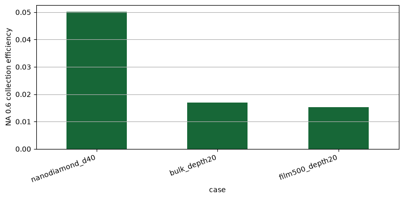
Reference & Related Tidy3D Official Document
Reference for NV Center Properties
- J. Hadden et al., “Micro-concave waveguide antenna for high photon extraction from nitrogen vacancy centers in nanodiamond,” Scientific Reports 5, 12013 (2015). https://www.nature.com/articles/srep12013
- I. H. Malitson, “Interspecimen Comparison of the Refractive Index of Fused Silica,” JOSA 55, 1205–1209 (1965).
https://opg.optica.org/josa/abstract.cfm?uri=josa-55-10-1205 - F. Peter diamond dispersion dataset as curated by RefractiveIndex.INFO; reported wavelength range 0.226–0.760 µm.
https://refractiveindex.info/?shelf=main&book=C&page=Peter - M. N. Polyanskiy, “Refractiveindex.info database of optical constants,” Scientific Data 11, 94 (2024).
https://www.nature.com/articles/s41597-023-02898-2
Tidy3D Official Document
- Point dipole and arbitrary-direction helper:
https://docs.flexcompute.com/projects/tidy3d/en/latest/api/_autosummary/tidy3d.PointDipole.html - Field projection angle monitor:
https://docs.flexcompute.com/projects/tidy3d/en/latest/api/_autosummary/tidy3d.FieldProjectionAngleMonitor.html - Flux monitor:
https://docs.flexcompute.com/projects/tidy3d/en/latest/api/_autosummary/tidy3d.FluxMonitor.html - Simulation and
normalize_index:
https://docs.flexcompute.com/projects/tidy3d/en/latest/api/_autosummary/tidy3d.Simulation.html - Mesh override:
https://docs.flexcompute.com/projects/tidy3d/en/latest/api/discretization/_autosummary/tidy3d.MeshOverrideStructure.html - Sellmeier medium:
https://docs.flexcompute.com/projects/tidy3d/en/latest/api/_autosummary/tidy3d.Sellmeier.html - Batch execution:
https://docs.flexcompute.com/projects/tidy3d/en/latest/api/_autosummary/tidy3d.web.api.container.Batch.html - BatchData:
https://docs.flexcompute.com/projects/tidy3d/en/latest/api/_autosummary/tidy3d.web.BatchData.html

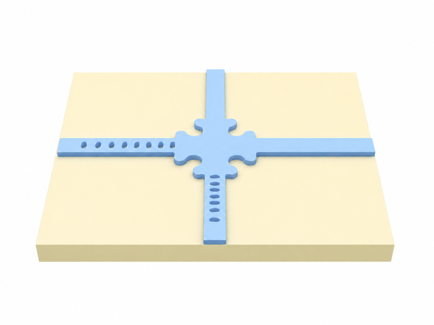


 TERMS & CONDITIONS


 How the process works:
 Try this real URL to see an example: