





Author: Sayan Gangopadhyay, University of Waterloo
Note: the total cost of running the entire notebook is about 25 FlexCredits.
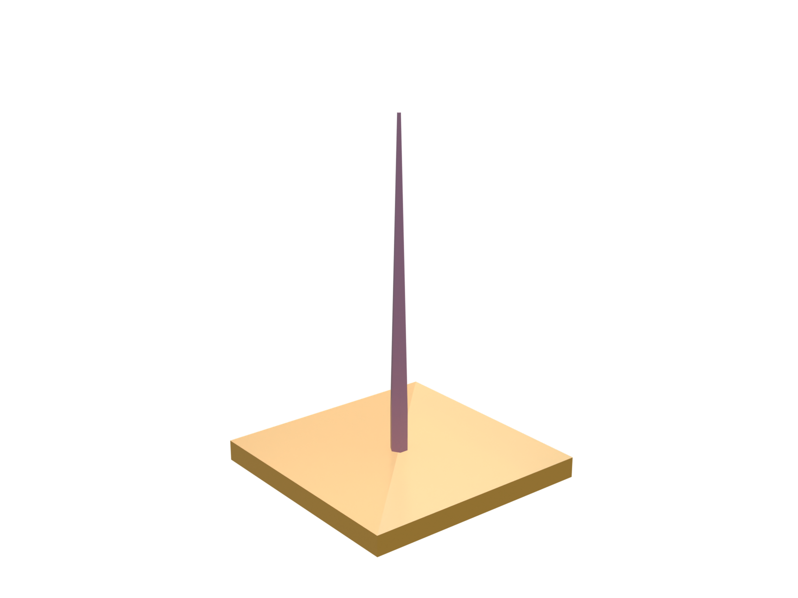
Semiconductor nanowires with embedded quantum dots are a promising platform for bright single-photon sources. The emitter is placed on the axis of a high index nanowire waveguide, which funnels its spontaneous emission into the fundamental guided mode. A long taper expands the mode adiabatically toward a truncated tip, producing a directive far field, while a metallic mirror below the wire redirects the downward emission. The interference between the direct and reflected fields modulates the local density of states, so the emission rate depends strongly on the emitter height above the mirror.
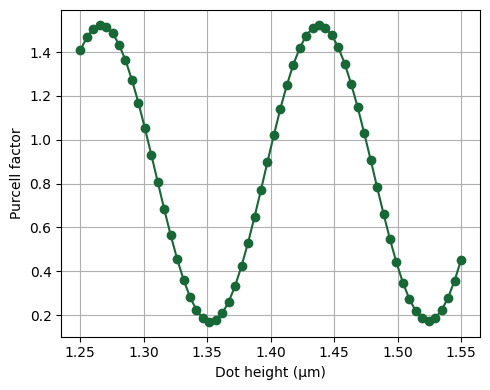
In this notebook, we model a hexagonal InP nanowire standing on a gold mirror covered by a thin $\text{SiO}_2$ spacer. The quantum dot is represented by a PointDipole source, and the power it emits is measured with a closed FluxMonitor box surrounding it. Using a Batch, we sweep the dot height above the mirror over 60 values and compute the Purcell factor as the ratio between the dipole power emitted in the device and in bulk InP.
import numpy as np
import matplotlib.pyplot as plt

import tidy3d as td
import tidy3d.web as web
from tidy3d.log import set_warn_once

set_warn_once(True)  # show each unique warning only once
Simulation Parameters
We first define the geometry, material, and numerical parameters. All spatial dimensions are in micrometers. The nanowire consists of a straight hexagonal section of height $H$ and a long taper of height $H_{\text{taper}}$ that narrows from a circumradius $R$ at the base to $R_{\text{tip}}$ at the truncated tip. The wire stands on a 10 nm $\text{SiO}_2$ layer over a 1 $\mu m$ thick gold film.
# ============================================================
# USER PARAMETERS
# Tidy3D spatial units are micrometers.
# ============================================================

wavelength0 = 0.90       # central vacuum wavelength [um]

H = 2.0                  # straight-section height [um]
H_taper=13.922           # taper height [um]
#H_taper=5.5
R = 0.1515                # base hexagon circumradius [um]
R_tip = 0.030             # truncated-tip circumradius: 30 nm [um]

msize = 4.0              # lateral size of Au and oxide [um]

t_gold = 1.00            # gold thickness: 1 um
t_oxide = 0.010           # oxide thickness: 10 nm [um]


monitor_above_tip = 1.500

run_time = 2e-12         # 2 ps

n_nanowire = 3.44         # nondispersive InP approximation
n_oxide = 1.45            # nondispersive SiO2 approximation

xy_air_padding = 0.0
bottom_air_padding = 0.0
top_air_padding = 0.8

monitor_span = msize       # adjust independently if desired

min_steps_per_wvl = 10
Next, we compute the source frequency, define the materials, and set the z coordinates of the material interfaces. InP and $\text{SiO}_2$ are modeled as nondispersive Medium objects, and gold uses the Johnson and Christy fit from the Tidy3D material library. The top surface of the gold film is at $z = 0$.
# ============================================================
# FREQUENCY
# ============================================================

freq0 = td.C_0 / wavelength0

# A moderately broadband pulse.
# Increase the denominator for a narrower source spectrum.
fwidth = freq0 / 10


# ============================================================
# MATERIALS
# ============================================================

air = td.Medium(name="air")

nanowire_medium = td.Medium(
    permittivity=n_nanowire**2,
    name="InP",
)

oxide_medium = td.Medium(
    permittivity=n_oxide**2,
    name="SiO2",
)

gold_medium = td.material_library["Au"]["JohnsonChristy1972"]


# ============================================================
# Z POSITIONS
#
# Gold top surface is defined as z = 0.
# ============================================================

z_gold_min = -t_gold
z_gold_max = 0.0

z_oxide_min = 0.0
z_oxide_max = t_oxide

z_wire_min = z_oxide_max
z_base_max = z_wire_min + H
z_tip = z_base_max + H_taper


z_monitor = z_tip + monitor_above_tip
Hexagonal Cross Section and Taper Angle
The function below returns the vertices of a regular hexagon of a given circumradius, used as the base of the PolySlab sections. In a PolySlab, the sidewall displacement occurs normal to each polygon edge, so the taper angle is set by the reduction of the apothem (the center to edge distance) rather than of the circumradius.
# ============================================================
# REGULAR HEXAGON
#
# R is the circumradius: distance from center to a vertex.
# rotation = pi/6 produces horizontal upper/lower facets.
# ============================================================

def hexagon_vertices(
    radius: float,
    rotation: float = np.pi / 6,
) -> list[tuple[float, float]]:
    """Return counter-clockwise vertices of a regular hexagon."""
    angles = rotation + np.arange(6) * np.pi / 3

    return [
        (
            radius * np.cos(angle),
            radius * np.sin(angle),
        )
        for angle in angles
    ]


base_vertices = hexagon_vertices(R)


# ============================================================
# TAPER ANGLE
#
# PolySlab sidewall displacement occurs normal to each polygon
# side. For a regular hexagon:
#
#     apothem = circumradius * cos(pi/6)
#
# Therefore, the required reduction in apothem is used here,
# rather than directly using R - R_tip.
# ============================================================

apothem_base = R * np.cos(np.pi / 6)
apothem_tip = R_tip * np.cos(np.pi / 6)

taper_angle = np.arctan(
    (apothem_base - apothem_tip) / H_taper
)

print(f"Taper sidewall angle: {np.degrees(taper_angle):.3f} degrees")
Taper sidewall angle: 0.433 degrees
Simulation Set Up
The function below builds the complete Simulation for a given dot height. The quantum dot is modeled as a y-polarized PointDipole placed on the wire axis. The monitors include a small closed FluxMonitor box around the dipole that measures the total emitted power, a FluxMonitor plane above the tip for the upward flux, a FieldProjectionAngleMonitor for the far-field radiation pattern, a FieldMonitor cross section for field visualization, and a FieldTimeMonitor to verify that the fields decay by the end of the simulation. MeshOverrideStructure refinements resolve the 10 nm oxide layer, the nanowire cross section, and the dipole region. Since the dipole is centered and y-polarized, symmetry planes at $x = 0$ (even) and $y = 0$ (odd) reduce the computational cost by a factor of 4.
# ============================================================
# STRUCTURES
# ============================================================
def make_sim(dot_height):
    z_dipole_above_mirror = dot_height
    z_dipole = z_dipole_above_mirror
    # Extend the gold film 2 um beyond the simulation bottom so it
    # passes all the way through the PML instead of ending at the
    # domain edge.
    gold = td.Structure(
        geometry=td.Box.from_bounds(
            rmin=(-msize, -msize, z_gold_min - 2 * t_gold),
            rmax=(msize, msize, z_gold_max),
        ),
        medium=gold_medium,
        name="gold_substrate",
    )


    oxide = td.Structure(
        geometry=td.Box(
            center=(
                0,
                0,
                0.5 * (z_oxide_min + z_oxide_max),
            ),
            size=(
                2*msize,
                2*msize,
                t_oxide,
            ),
        ),
        medium=oxide_medium,
        name="oxide_layer",
    )


    straight_section = td.Structure(
        geometry=td.PolySlab(
            vertices=base_vertices,
            axis=2,
            slab_bounds=(
                z_wire_min,
                z_base_max,
            ),
            sidewall_angle=0.0,
            reference_plane="bottom",
        ),
        medium=nanowire_medium,
        name="straight_hexagonal_section",
    )


    taper_section = td.Structure(
        geometry=td.PolySlab(
            vertices=base_vertices,
            axis=2,
            slab_bounds=(
                z_base_max,
                z_tip,
            ),
            sidewall_angle=taper_angle,
            reference_plane="bottom",
        ),
        medium=nanowire_medium,
        name="hexagonal_taper",
    )


    # ============================================================
    # SOURCE
    #
    # A +Ey and -Ey point dipole differ only by a global pi phase.
    # This does not change intensity, flux, Purcell factor, or the
    # required symmetry.
    # ============================================================

    source_time = td.GaussianPulse(
        freq0=freq0,
        fwidth=fwidth,
        remove_dc_component=True,
    )

    dipole = td.PointDipole(
        center=(0, 0, z_dipole),
        polarization="Ey",
        source_time=source_time,
        name="y_dipole",
    )


    # ============================================================
    # MONITORS
    #
    # The plane is 1.5 um above the truncated tip.
    # ============================================================
    # ============================================================
    # FAR-FIELD PROJECTION MONITOR
    #
    # theta = 0 corresponds to propagation along +z.
    # theta = pi/2 corresponds to grazing propagation.
    # phi is measured azimuthally from +x toward +y.
    # ============================================================

    theta_ff = np.linspace(0, np.pi / 2, 181)
    phi_ff = np.linspace(0, 2 * np.pi, 361)

    ff_box_bottom = t_oxide + 0.050
    ff_box_top = z_monitor

    ff_box_center_z = 0.5 * (ff_box_bottom + ff_box_top)
    ff_box_span_z = ff_box_top - ff_box_bottom

    far_field_monitor = td.FieldProjectionAngleMonitor(
        center=(0, 0, ff_box_center_z),
        size=(monitor_span, monitor_span, ff_box_span_z),
        freqs=[freq0],
        name="far_field_box",
        theta=theta_ff,
        phi=phi_ff,
        custom_origin=(0, 0, z_dipole),
        exclude_surfaces=("z-",),
        proj_distance=1000 * wavelength0,
        far_field_approx=True,
        interval_space=(2, 2, 2),
    )
    x_min, x_max = -3, 3
    y_min, y_max = 0, 0
    z_min = 0
    z_max = z_tip

    field_monitor = td.FieldMonitor(
        center=(
            (x_min + x_max) / 2,
            (y_min + y_max) / 2,
            (z_min + z_max) / 2,
        ),
        size=(
            x_max - x_min,
            0,
            z_max - z_min,
        ),
        freqs=[freq0],
        fields=[
            "Ex",
            "Ey",
            "Ez",
            "Hx",
            "Hy",
            "Hz",
        ],
        name="field_cross_sec",
    )

    flux_monitor = td.FluxMonitor(
        center=(0, 0, z_monitor),
        size=(monitor_span, monitor_span, 0),
        freqs=[freq0],
        normal_dir="+",
        name="upward_flux",
    )
    purcell_monitor = td.FluxMonitor(
        center=(0, 0, z_dipole),
        size=(0.20, 0.20, 0.20),
        freqs=[freq0],
        name="dipole_power",
    )

    # Optional time-domain monitor for checking whether fields decay.
    decay_monitor = td.FieldTimeMonitor(
        center=(0, 0, z_monitor),
        size=(0, 0, 0),
        fields=["Ey"],
        start=0,
        stop=run_time,
        interval=10,
        name="field_decay",
    )


    # ============================================================
    # SIMULATION DOMAIN
    # ============================================================

    sim_x = msize + 2 * xy_air_padding
    sim_y = msize + 2 * xy_air_padding

    z_sim_min = z_gold_min - bottom_air_padding
    z_sim_max = z_monitor + top_air_padding

    sim_z = z_sim_max - z_sim_min
    sim_center_z = 0.5 * (z_sim_min + z_sim_max)


    # ============================================================
    # MESH
    #
    # The 10 nm oxide requires explicit refinement in z. Here the
    # oxide and nearby interfaces receive a 5 nm maximum cell size.
    # ============================================================

    oxide_mesh_override = td.MeshOverrideStructure(
        geometry=td.Box(
            center=(0, 0, t_oxide / 2),
            size=(msize, msize, t_oxide + 0.040),
        ),
        dl=(None, None, 0.005),
        name="oxide_z_mesh",
    )


    nanowire_mesh_override = td.MeshOverrideStructure(
        geometry=td.Box(
            center=(
                0,
                0,
                0.5 * (z_wire_min + z_tip),
            ),
            size=(
                2 * R + 0.2,
                2 * R + 0.2,
                z_tip - z_wire_min + 0.1,
            ),
        ),
        dl=(0.01, 0.01, 0.01),
        name="nanowire_mesh",
        priority=1,
    )

    dot_mesh_override = td.MeshOverrideStructure(
        geometry=td.Box(
            center=(0, 0, z_dipole),
            size=(0.050, 0.050, 0.050),
        ),
        dl=(None, None, 0.005),
        name="oxide_z_mesh",
        priority=2,
    )


    grid_spec = td.GridSpec.auto(
        wavelength=wavelength0,
        min_steps_per_wvl=min_steps_per_wvl,
        override_structures=[
            oxide_mesh_override,
            nanowire_mesh_override,
            dot_mesh_override,
        ],
    )


    # ============================================================
    # SYMMETRY
    #
    # For a centered y-oriented electric dipole:
    #
    # x = 0 plane:
    #   Ey is tangential and even -> PMC/even symmetry -> +1
    #
    # y = 0 plane:
    #   Ey is normal and even     -> PEC/odd symmetry  -> -1
    #
    # Tuple order is (x, y, z).
    # ============================================================

    symmetry = (1, -1, 0)


    # ============================================================
    # COMPLETE SIMULATION
    # ============================================================

    sim = td.Simulation(
        center=(0, 0, sim_center_z),
        size=(sim_x, sim_y, sim_z),

        medium=air,

        structures=[
            gold,
            oxide,
            straight_section,
            taper_section,
        ],

        sources=[dipole],

        monitors=[
            field_monitor,
            purcell_monitor,
            far_field_monitor,
            flux_monitor,
            decay_monitor,
        ],

        grid_spec=grid_spec,

        boundary_spec=td.BoundarySpec.all_sides(
            boundary=td.PML()
        ),

        symmetry=symmetry,

        run_time=run_time,
        shutoff=1e-6,
    )
    return sim
Parameter Sweep
We sweep the dot height from 1.25 to 1.55 $\mu m$ in 60 steps, creating one simulation per height. Before uploading, validate_pre_upload() checks each simulation locally and catches setup problems early.
# ============================================================
# MAKE A DICTIONARY OF SIMS
# ============================================================
dot_heights = np.linspace(1.250,1.550,60)

simulations = {
    f"D_{dot_height:.3f}": make_sim(dot_height)
    for dot_height in dot_heights
}
# ============================================================
# LOCAL VALIDATION
# ============================================================

for task_name, sim in simulations.items():
    print(f"Validating {task_name}...")
    sim.validate_pre_upload()

print("All simulations validated successfully.")
Validating D_1.250...
Validating D_1.255...
Validating D_1.260...
Validating D_1.265...
Validating D_1.270...
Validating D_1.275...
Validating D_1.281...
Validating D_1.286...
Validating D_1.291...
Validating D_1.296...
Validating D_1.301...
Validating D_1.306...
Validating D_1.311...
Validating D_1.316...
Validating D_1.321...
Validating D_1.326...
Validating D_1.331...
Validating D_1.336...
Validating D_1.342...
Validating D_1.347...
Validating D_1.352...
Validating D_1.357...
Validating D_1.362...
Validating D_1.367...
Validating D_1.372...
Validating D_1.377...
Validating D_1.382...
Validating D_1.387...
Validating D_1.392...
Validating D_1.397...
Validating D_1.403...
Validating D_1.408...
Validating D_1.413...
Validating D_1.418...
Validating D_1.423...
Validating D_1.428...
Validating D_1.433...
Validating D_1.438...
Validating D_1.443...
Validating D_1.448...
Validating D_1.453...
Validating D_1.458...
Validating D_1.464...
Validating D_1.469...
Validating D_1.474...
Validating D_1.479...
Validating D_1.484...
Validating D_1.489...
Validating D_1.494...
Validating D_1.499...
Validating D_1.504...
Validating D_1.509...
Validating D_1.514...
Validating D_1.519...
Validating D_1.525...
Validating D_1.530...
Validating D_1.535...
Validating D_1.540...
Validating D_1.545...
Validating D_1.550...
All simulations validated successfully.
Geometry Visualization
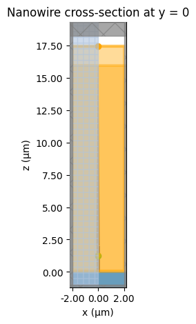
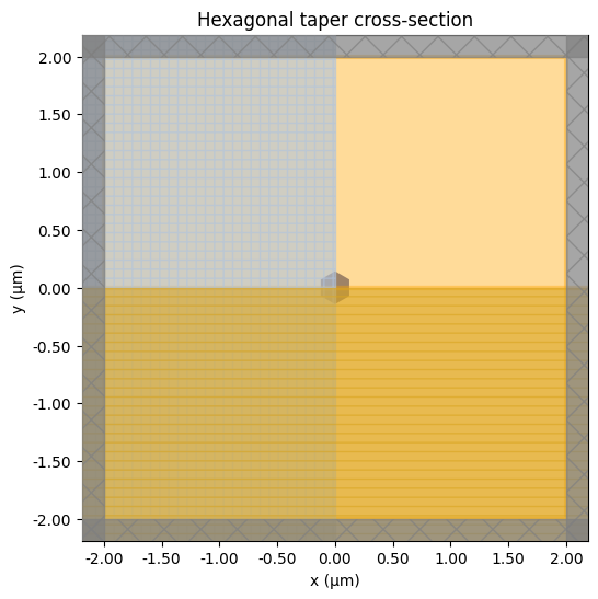
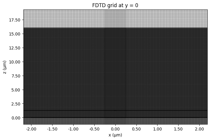
Before running the sweep, we inspect the first simulation: the nanowire cross section, the hexagonal taper cross section, and the FDTD grid.
# ============================================================
# PLOT GEOMETRY
# ============================================================
first_sim = next(iter(simulations.values())) # this is the first sim in the dictionary
fig, ax = plt.subplots(figsize=(8, 5))
first_sim.plot(y=0, ax=ax)
ax.set_title("Nanowire cross-section at y = 0")
plt.show()

fig, ax = plt.subplots(figsize=(6, 6))
first_sim.plot(z=z_base_max + 0.5 * H, ax=ax)
ax.set_title("Hexagonal taper cross-section")
plt.show()

fig, ax = plt.subplots(figsize=(8, 5))
first_sim.plot_grid(y=0, ax=ax)
ax.set_title("FDTD grid at y = 0")
plt.show()
Cost Estimation
The simulations are grouped in a Batch that uploads and runs them together. The estimate_cost() method returns the maximum FlexCredit cost of the whole batch before it starts. The real billed cost is usually considerably lower because the simulations terminate early once the fields decay below the shutoff threshold.
# ============================================================
# CREATE JOB AND ESTIMATE COST
# ============================================================

batch = web.Batch(simulations=simulations)

print(batch.estimate_cost())
11:58:34 -03 Maximum FlexCredit cost: 155.929 for the whole batch.
155.9289782898351
Running the Batch
Batch.run() uploads all simulations, monitors their progress, and downloads the results when they complete.
# ============================================================
# RUN
# ============================================================

batch_data = batch.run(
    path_dir="hexagonal_nanowire_on_gold"
)
Output()
11:58:42 -03 Started working on Batch containing 60 tasks.
12:00:36 -03 Maximum FlexCredit cost: 155.929 for the whole batch.
             Use 'Batch.real_cost()' to get the billed FlexCredit cost after
             completion.
Output()
12:21:37 -03 Batch complete.
The solver log warns about a dispersive medium (the gold) extending into the PML. This is expected and safe in this case: the gold film is optically thick, so the fields decay inside it and do not penetrate the PML region behind it.
Purcell Factor Calculation
The Purcell factor is defined as $F_p = P_{\text{device}} / P_{\text{bulk}}$, where $P_{\text{device}}$ is the power emitted by the dipole inside the structure and $P_{\text{bulk}}$ is the power emitted by the same dipole in homogeneous InP, computed analytically as
$$P_{\text{bulk}} = \frac{\omega^2}{12 \pi} \frac{\mu_0 n}{c}.$$
When symmetry planes are present, dipole images are included for each plane, so $P_{\text{bulk}}$ must be multiplied by $2^{2 N_{\text{sym}}}$, where $N_{\text{sym}}$ is the number of symmetry planes.
# ============================================================
# BULK DIPOLE POWER (ANALYTIC)
#
# Power emitted by the same dipole in homogeneous InP,
# corrected for the dipole images introduced by the
# symmetry planes.
# ============================================================

P_bulk = ((2 * np.pi * freq0) ** 2 / (12 * np.pi)) * (td.MU_0 * n_nanowire / td.C_0)
P_bulk = P_bulk * 2 ** (2 * np.sum(np.abs(first_sim.symmetry)))

print(f"P_bulk = {P_bulk:.6e}")
P_bulk = 2.680727e+04
For each simulation in the batch, we take the dipole power from the flux box monitor and normalize it by the bulk reference.
# ============================================================
# EXTRACT ACTUAL PURCELL FACTORS
# ============================================================

purcells = []

for dot_height, task_name in zip(
    dot_heights,
    simulations.keys(),
):

    sim_data = batch_data[task_name]

    P_device = float(
        sim_data["dipole_power"].flux.sel(
            f=freq0,
            method="nearest",
        )
    )

    purcell = P_device / P_bulk
    purcells.append(purcell)

    print(
        f"Dot height = {dot_height:.3f} µm, "
        f"Purcell = {purcell:.6f}"
    )

purcells = np.array(purcells)
Dot height = 1.250 µm, Purcell = 1.407922
Dot height = 1.255 µm, Purcell = 1.467918
Dot height = 1.260 µm, Purcell = 1.507342
Dot height = 1.265 µm, Purcell = 1.524628
Dot height = 1.270 µm, Purcell = 1.516392
Dot height = 1.275 µm, Purcell = 1.487461
Dot height = 1.281 µm, Purcell = 1.434381
Dot height = 1.286 µm, Purcell = 1.363479
Dot height = 1.291 µm, Purcell = 1.273250
Dot height = 1.296 µm, Purcell = 1.169655
Dot height = 1.301 µm, Purcell = 1.054108
Dot height = 1.306 µm, Purcell = 0.932519
Dot height = 1.311 µm, Purcell = 0.807763
Dot height = 1.316 µm, Purcell = 0.683838
Dot height = 1.321 µm, Purcell = 0.565789
Dot height = 1.326 µm, Purcell = 0.457001
Dot height = 1.331 µm, Purcell = 0.361717
Dot height = 1.336 µm, Purcell = 0.282629
Dot height = 1.342 µm, Purcell = 0.223002
Dot height = 1.347 µm, Purcell = 0.184572
Dot height = 1.352 µm, Purcell = 0.168912
Dot height = 1.357 µm, Purcell = 0.176630
Dot height = 1.362 µm, Purcell = 0.207228
Dot height = 1.367 µm, Purcell = 0.260496
Dot height = 1.372 µm, Purcell = 0.333511
Dot height = 1.377 µm, Purcell = 0.425201
Dot height = 1.382 µm, Purcell = 0.530375
Dot height = 1.387 µm, Purcell = 0.648082
Dot height = 1.392 µm, Purcell = 0.770889
Dot height = 1.397 µm, Purcell = 0.898345
Dot height = 1.403 µm, Purcell = 1.021574
Dot height = 1.408 µm, Purcell = 1.141229
Dot height = 1.413 µm, Purcell = 1.248013
Dot height = 1.418 µm, Purcell = 1.342607
Dot height = 1.423 µm, Purcell = 1.417494
Dot height = 1.428 µm, Purcell = 1.475826
Dot height = 1.433 µm, Purcell = 1.509801
Dot height = 1.438 µm, Purcell = 1.522528
Dot height = 1.443 µm, Purcell = 1.511137
Dot height = 1.448 µm, Purcell = 1.476930
Dot height = 1.453 µm, Purcell = 1.421451
Dot height = 1.458 µm, Purcell = 1.345774
Dot height = 1.464 µm, Purcell = 1.252828
Dot height = 1.469 µm, Purcell = 1.147580
Dot height = 1.474 µm, Purcell = 1.030137
Dot height = 1.479 µm, Purcell = 0.908843
Dot height = 1.484 µm, Purcell = 0.783521
Dot height = 1.489 µm, Purcell = 0.661923
Dot height = 1.494 µm, Purcell = 0.545201
Dot height = 1.499 µm, Purcell = 0.440072
Dot height = 1.504 µm, Purcell = 0.347761
Dot height = 1.509 µm, Purcell = 0.273340
Dot height = 1.514 µm, Purcell = 0.217969
Dot height = 1.519 µm, Purcell = 0.184615
Dot height = 1.525 µm, Purcell = 0.173829
Dot height = 1.530 µm, Purcell = 0.186449
Dot height = 1.535 µm, Purcell = 0.221937
Dot height = 1.540 µm, Purcell = 0.279112
Dot height = 1.545 µm, Purcell = 0.356188
Dot height = 1.550 µm, Purcell = 0.450247
Results
Finally, we plot the Purcell factor as a function of the dot height above the mirror. The oscillation reflects the standing wave formed between the emitter and the gold mirror.
# ============================================================
# PLOT
# ============================================================
plt.figure(figsize=(5, 4))
plt.plot(dot_heights, purcells, "o-")
plt.xlabel("Dot height (µm)")
plt.ylabel("Purcell factor")
plt.grid(True)
plt.tight_layout()
plt.savefig("purcell_vs_dot_height_mirror.pdf", bbox_inches="tight")
plt.show()
Real Cost
After completion, we query the real billed FlexCredit cost of each task in the batch.
total_cost = 0

for task_name, job in batch.jobs.items():
    cost = web.real_cost(job.task_id)
    total_cost += cost
    print(f"{task_name}: {cost:.3f} FlexCredits")

print(f"\nTotal actual cost: {total_cost:.3f} FlexCredits")
12:22:09 -03 Billed flex credit cost: 0.421.
             Note: the task cost pro-rated due to early shutoff was below the
             minimum threshold, due to fast shutoff. Decreasing the simulation
             'run_time' should decrease the estimated, and correspondingly the
             billed cost of such tasks.
D_1.250: 0.421 FlexCredits
12:22:10 -03 Billed flex credit cost: 0.421.
             Note: the task cost pro-rated due to early shutoff was below the
             minimum threshold, due to fast shutoff. Decreasing the simulation
             'run_time' should decrease the estimated, and correspondingly the
             billed cost of such tasks.
D_1.255: 0.421 FlexCredits
Billed flex credit cost: 0.421.
             Note: the task cost pro-rated due to early shutoff was below the
             minimum threshold, due to fast shutoff. Decreasing the simulation
             'run_time' should decrease the estimated, and correspondingly the
             billed cost of such tasks.
D_1.260: 0.421 FlexCredits
12:22:11 -03 Billed flex credit cost: 0.421.
             Note: the task cost pro-rated due to early shutoff was below the
             minimum threshold, due to fast shutoff. Decreasing the simulation
             'run_time' should decrease the estimated, and correspondingly the
             billed cost of such tasks.
D_1.265: 0.421 FlexCredits
Billed flex credit cost: 0.427.
             Note: the task cost pro-rated due to early shutoff was below the
             minimum threshold, due to fast shutoff. Decreasing the simulation
             'run_time' should decrease the estimated, and correspondingly the
             billed cost of such tasks.
D_1.270: 0.427 FlexCredits
12:22:12 -03 Billed flex credit cost: 0.427.
             Note: the task cost pro-rated due to early shutoff was below the
             minimum threshold, due to fast shutoff. Decreasing the simulation
             'run_time' should decrease the estimated, and correspondingly the
             billed cost of such tasks.
D_1.275: 0.427 FlexCredits
Billed flex credit cost: 0.427.
             Note: the task cost pro-rated due to early shutoff was below the
             minimum threshold, due to fast shutoff. Decreasing the simulation
             'run_time' should decrease the estimated, and correspondingly the
             billed cost of such tasks.
D_1.281: 0.427 FlexCredits
12:22:13 -03 Billed flex credit cost: 0.427.
             Note: the task cost pro-rated due to early shutoff was below the
             minimum threshold, due to fast shutoff. Decreasing the simulation
             'run_time' should decrease the estimated, and correspondingly the
             billed cost of such tasks.
D_1.286: 0.427 FlexCredits
12:22:15 -03 Billed flex credit cost: 0.427.
             Note: the task cost pro-rated due to early shutoff was below the
             minimum threshold, due to fast shutoff. Decreasing the simulation
             'run_time' should decrease the estimated, and correspondingly the
             billed cost of such tasks.
D_1.291: 0.427 FlexCredits
12:22:16 -03 Billed flex credit cost: 0.427.
             Note: the task cost pro-rated due to early shutoff was below the
             minimum threshold, due to fast shutoff. Decreasing the simulation
             'run_time' should decrease the estimated, and correspondingly the
             billed cost of such tasks.
D_1.296: 0.427 FlexCredits
Billed flex credit cost: 0.427.
             Note: the task cost pro-rated due to early shutoff was below the
             minimum threshold, due to fast shutoff. Decreasing the simulation
             'run_time' should decrease the estimated, and correspondingly the
             billed cost of such tasks.
D_1.301: 0.427 FlexCredits
12:22:17 -03 Billed flex credit cost: 0.427.
             Note: the task cost pro-rated due to early shutoff was below the
             minimum threshold, due to fast shutoff. Decreasing the simulation
             'run_time' should decrease the estimated, and correspondingly the
             billed cost of such tasks.
D_1.306: 0.427 FlexCredits
Billed flex credit cost: 0.427.
             Note: the task cost pro-rated due to early shutoff was below the
             minimum threshold, due to fast shutoff. Decreasing the simulation
             'run_time' should decrease the estimated, and correspondingly the
             billed cost of such tasks.
D_1.311: 0.427 FlexCredits
12:22:18 -03 Billed flex credit cost: 0.427.
             Note: the task cost pro-rated due to early shutoff was below the
             minimum threshold, due to fast shutoff. Decreasing the simulation
             'run_time' should decrease the estimated, and correspondingly the
             billed cost of such tasks.
D_1.316: 0.427 FlexCredits
12:22:19 -03 Billed flex credit cost: 0.427.
             Note: the task cost pro-rated due to early shutoff was below the
             minimum threshold, due to fast shutoff. Decreasing the simulation
             'run_time' should decrease the estimated, and correspondingly the
             billed cost of such tasks.
D_1.321: 0.427 FlexCredits
Billed flex credit cost: 0.427.
             Note: the task cost pro-rated due to early shutoff was below the
             minimum threshold, due to fast shutoff. Decreasing the simulation
             'run_time' should decrease the estimated, and correspondingly the
             billed cost of such tasks.
D_1.326: 0.427 FlexCredits
12:22:20 -03 Billed flex credit cost: 0.427.
             Note: the task cost pro-rated due to early shutoff was below the
             minimum threshold, due to fast shutoff. Decreasing the simulation
             'run_time' should decrease the estimated, and correspondingly the
             billed cost of such tasks.
D_1.331: 0.427 FlexCredits
Billed flex credit cost: 0.427.
             Note: the task cost pro-rated due to early shutoff was below the
             minimum threshold, due to fast shutoff. Decreasing the simulation
             'run_time' should decrease the estimated, and correspondingly the
             billed cost of such tasks.
D_1.336: 0.427 FlexCredits
12:22:21 -03 Billed flex credit cost: 0.427.
             Note: the task cost pro-rated due to early shutoff was below the
             minimum threshold, due to fast shutoff. Decreasing the simulation
             'run_time' should decrease the estimated, and correspondingly the
             billed cost of such tasks.
D_1.342: 0.427 FlexCredits
12:22:22 -03 Billed flex credit cost: 0.427.
             Note: the task cost pro-rated due to early shutoff was below the
             minimum threshold, due to fast shutoff. Decreasing the simulation
             'run_time' should decrease the estimated, and correspondingly the
             billed cost of such tasks.
D_1.347: 0.427 FlexCredits
12:22:23 -03 Billed flex credit cost: 0.427.
             Note: the task cost pro-rated due to early shutoff was below the
             minimum threshold, due to fast shutoff. Decreasing the simulation
             'run_time' should decrease the estimated, and correspondingly the
             billed cost of such tasks.
D_1.352: 0.427 FlexCredits
12:22:24 -03 Billed flex credit cost: 0.427.
             Note: the task cost pro-rated due to early shutoff was below the
             minimum threshold, due to fast shutoff. Decreasing the simulation
             'run_time' should decrease the estimated, and correspondingly the
             billed cost of such tasks.
D_1.357: 0.427 FlexCredits
Billed flex credit cost: 0.421.
             Note: the task cost pro-rated due to early shutoff was below the
             minimum threshold, due to fast shutoff. Decreasing the simulation
             'run_time' should decrease the estimated, and correspondingly the
             billed cost of such tasks.
D_1.362: 0.421 FlexCredits
12:22:25 -03 Billed flex credit cost: 0.421.
             Note: the task cost pro-rated due to early shutoff was below the
             minimum threshold, due to fast shutoff. Decreasing the simulation
             'run_time' should decrease the estimated, and correspondingly the
             billed cost of such tasks.
D_1.367: 0.421 FlexCredits
Billed flex credit cost: 0.421.
             Note: the task cost pro-rated due to early shutoff was below the
             minimum threshold, due to fast shutoff. Decreasing the simulation
             'run_time' should decrease the estimated, and correspondingly the
             billed cost of such tasks.
D_1.372: 0.421 FlexCredits
12:22:26 -03 Billed flex credit cost: 0.421.
             Note: the task cost pro-rated due to early shutoff was below the
             minimum threshold, due to fast shutoff. Decreasing the simulation
             'run_time' should decrease the estimated, and correspondingly the
             billed cost of such tasks.
D_1.377: 0.421 FlexCredits
Billed flex credit cost: 0.421.
             Note: the task cost pro-rated due to early shutoff was below the
             minimum threshold, due to fast shutoff. Decreasing the simulation
             'run_time' should decrease the estimated, and correspondingly the
             billed cost of such tasks.
D_1.382: 0.421 FlexCredits
12:22:27 -03 Billed flex credit cost: 0.421.
             Note: the task cost pro-rated due to early shutoff was below the
             minimum threshold, due to fast shutoff. Decreasing the simulation
             'run_time' should decrease the estimated, and correspondingly the
             billed cost of such tasks.
D_1.387: 0.421 FlexCredits
12:22:28 -03 Billed flex credit cost: 0.421.
             Note: the task cost pro-rated due to early shutoff was below the
             minimum threshold, due to fast shutoff. Decreasing the simulation
             'run_time' should decrease the estimated, and correspondingly the
             billed cost of such tasks.
D_1.392: 0.421 FlexCredits
12:22:29 -03 Billed flex credit cost: 0.421.
             Note: the task cost pro-rated due to early shutoff was below the
             minimum threshold, due to fast shutoff. Decreasing the simulation
             'run_time' should decrease the estimated, and correspondingly the
             billed cost of such tasks.
D_1.397: 0.421 FlexCredits
12:22:30 -03 Billed flex credit cost: 0.421.
             Note: the task cost pro-rated due to early shutoff was below the
             minimum threshold, due to fast shutoff. Decreasing the simulation
             'run_time' should decrease the estimated, and correspondingly the
             billed cost of such tasks.
D_1.403: 0.421 FlexCredits
12:22:31 -03 Billed flex credit cost: 0.421.
             Note: the task cost pro-rated due to early shutoff was below the
             minimum threshold, due to fast shutoff. Decreasing the simulation
             'run_time' should decrease the estimated, and correspondingly the
             billed cost of such tasks.
D_1.408: 0.421 FlexCredits
12:22:32 -03 Billed flex credit cost: 0.421.
             Note: the task cost pro-rated due to early shutoff was below the
             minimum threshold, due to fast shutoff. Decreasing the simulation
             'run_time' should decrease the estimated, and correspondingly the
             billed cost of such tasks.
D_1.413: 0.421 FlexCredits
Billed flex credit cost: 0.427.
             Note: the task cost pro-rated due to early shutoff was below the
             minimum threshold, due to fast shutoff. Decreasing the simulation
             'run_time' should decrease the estimated, and correspondingly the
             billed cost of such tasks.
D_1.418: 0.427 FlexCredits
12:22:33 -03 Billed flex credit cost: 0.427.
             Note: the task cost pro-rated due to early shutoff was below the
             minimum threshold, due to fast shutoff. Decreasing the simulation
             'run_time' should decrease the estimated, and correspondingly the
             billed cost of such tasks.
D_1.423: 0.427 FlexCredits
Billed flex credit cost: 0.427.
             Note: the task cost pro-rated due to early shutoff was below the
             minimum threshold, due to fast shutoff. Decreasing the simulation
             'run_time' should decrease the estimated, and correspondingly the
             billed cost of such tasks.
D_1.428: 0.427 FlexCredits
12:22:34 -03 Billed flex credit cost: 0.427.
             Note: the task cost pro-rated due to early shutoff was below the
             minimum threshold, due to fast shutoff. Decreasing the simulation
             'run_time' should decrease the estimated, and correspondingly the
             billed cost of such tasks.
D_1.433: 0.427 FlexCredits
12:22:35 -03 Billed flex credit cost: 0.427.
             Note: the task cost pro-rated due to early shutoff was below the
             minimum threshold, due to fast shutoff. Decreasing the simulation
             'run_time' should decrease the estimated, and correspondingly the
             billed cost of such tasks.
D_1.438: 0.427 FlexCredits
12:22:36 -03 Billed flex credit cost: 0.427.
             Note: the task cost pro-rated due to early shutoff was below the
             minimum threshold, due to fast shutoff. Decreasing the simulation
             'run_time' should decrease the estimated, and correspondingly the
             billed cost of such tasks.
D_1.443: 0.427 FlexCredits
12:22:37 -03 Billed flex credit cost: 0.427.
             Note: the task cost pro-rated due to early shutoff was below the
             minimum threshold, due to fast shutoff. Decreasing the simulation
             'run_time' should decrease the estimated, and correspondingly the
             billed cost of such tasks.
D_1.448: 0.427 FlexCredits
12:22:38 -03 Billed flex credit cost: 0.427.
             Note: the task cost pro-rated due to early shutoff was below the
             minimum threshold, due to fast shutoff. Decreasing the simulation
             'run_time' should decrease the estimated, and correspondingly the
             billed cost of such tasks.
D_1.453: 0.427 FlexCredits
12:22:39 -03 Billed flex credit cost: 0.427.
             Note: the task cost pro-rated due to early shutoff was below the
             minimum threshold, due to fast shutoff. Decreasing the simulation
             'run_time' should decrease the estimated, and correspondingly the
             billed cost of such tasks.
D_1.458: 0.427 FlexCredits
Billed flex credit cost: 0.427.
             Note: the task cost pro-rated due to early shutoff was below the
             minimum threshold, due to fast shutoff. Decreasing the simulation
             'run_time' should decrease the estimated, and correspondingly the
             billed cost of such tasks.
D_1.464: 0.427 FlexCredits
12:22:40 -03 Billed flex credit cost: 0.427.
             Note: the task cost pro-rated due to early shutoff was below the
             minimum threshold, due to fast shutoff. Decreasing the simulation
             'run_time' should decrease the estimated, and correspondingly the
             billed cost of such tasks.
D_1.469: 0.427 FlexCredits
12:22:41 -03 Billed flex credit cost: 0.427.
             Note: the task cost pro-rated due to early shutoff was below the
             minimum threshold, due to fast shutoff. Decreasing the simulation
             'run_time' should decrease the estimated, and correspondingly the
             billed cost of such tasks.
D_1.474: 0.427 FlexCredits
12:22:42 -03 Billed flex credit cost: 0.427.
             Note: the task cost pro-rated due to early shutoff was below the
             minimum threshold, due to fast shutoff. Decreasing the simulation
             'run_time' should decrease the estimated, and correspondingly the
             billed cost of such tasks.
D_1.479: 0.427 FlexCredits
12:22:43 -03 Billed flex credit cost: 0.427.
             Note: the task cost pro-rated due to early shutoff was below the
             minimum threshold, due to fast shutoff. Decreasing the simulation
             'run_time' should decrease the estimated, and correspondingly the
             billed cost of such tasks.
D_1.484: 0.427 FlexCredits
Billed flex credit cost: 0.427.
             Note: the task cost pro-rated due to early shutoff was below the
             minimum threshold, due to fast shutoff. Decreasing the simulation
             'run_time' should decrease the estimated, and correspondingly the
             billed cost of such tasks.
D_1.489: 0.427 FlexCredits
12:22:44 -03 Billed flex credit cost: 0.427.
             Note: the task cost pro-rated due to early shutoff was below the
             minimum threshold, due to fast shutoff. Decreasing the simulation
             'run_time' should decrease the estimated, and correspondingly the
             billed cost of such tasks.
D_1.494: 0.427 FlexCredits
Billed flex credit cost: 0.427.
             Note: the task cost pro-rated due to early shutoff was below the
             minimum threshold, due to fast shutoff. Decreasing the simulation
             'run_time' should decrease the estimated, and correspondingly the
             billed cost of such tasks.
D_1.499: 0.427 FlexCredits
12:22:45 -03 Billed flex credit cost: 0.427.
             Note: the task cost pro-rated due to early shutoff was below the
             minimum threshold, due to fast shutoff. Decreasing the simulation
             'run_time' should decrease the estimated, and correspondingly the
             billed cost of such tasks.
D_1.504: 0.427 FlexCredits
12:22:46 -03 Billed flex credit cost: 0.427.
             Note: the task cost pro-rated due to early shutoff was below the
             minimum threshold, due to fast shutoff. Decreasing the simulation
             'run_time' should decrease the estimated, and correspondingly the
             billed cost of such tasks.
D_1.509: 0.427 FlexCredits
12:22:47 -03 Billed flex credit cost: 0.427.
             Note: the task cost pro-rated due to early shutoff was below the
             minimum threshold, due to fast shutoff. Decreasing the simulation
             'run_time' should decrease the estimated, and correspondingly the
             billed cost of such tasks.
D_1.514: 0.427 FlexCredits
Billed flex credit cost: 0.427.
             Note: the task cost pro-rated due to early shutoff was below the
             minimum threshold, due to fast shutoff. Decreasing the simulation
             'run_time' should decrease the estimated, and correspondingly the
             billed cost of such tasks.
D_1.519: 0.427 FlexCredits
12:22:48 -03 Billed flex credit cost: 0.427.
             Note: the task cost pro-rated due to early shutoff was below the
             minimum threshold, due to fast shutoff. Decreasing the simulation
             'run_time' should decrease the estimated, and correspondingly the
             billed cost of such tasks.
D_1.525: 0.427 FlexCredits
Billed flex credit cost: 0.427.
             Note: the task cost pro-rated due to early shutoff was below the
             minimum threshold, due to fast shutoff. Decreasing the simulation
             'run_time' should decrease the estimated, and correspondingly the
             billed cost of such tasks.
D_1.530: 0.427 FlexCredits
12:22:49 -03 Billed flex credit cost: 0.427.
             Note: the task cost pro-rated due to early shutoff was below the
             minimum threshold, due to fast shutoff. Decreasing the simulation
             'run_time' should decrease the estimated, and correspondingly the
             billed cost of such tasks.
D_1.535: 0.427 FlexCredits
Billed flex credit cost: 0.427.
             Note: the task cost pro-rated due to early shutoff was below the
             minimum threshold, due to fast shutoff. Decreasing the simulation
             'run_time' should decrease the estimated, and correspondingly the
             billed cost of such tasks.
D_1.540: 0.427 FlexCredits
12:22:50 -03 Billed flex credit cost: 0.427.
             Note: the task cost pro-rated due to early shutoff was below the
             minimum threshold, due to fast shutoff. Decreasing the simulation
             'run_time' should decrease the estimated, and correspondingly the
             billed cost of such tasks.
D_1.545: 0.427 FlexCredits
Billed flex credit cost: 0.427.
             Note: the task cost pro-rated due to early shutoff was below the
             minimum threshold, due to fast shutoff. Decreasing the simulation
             'run_time' should decrease the estimated, and correspondingly the
             billed cost of such tasks.
D_1.550: 0.427 FlexCredits

Total actual cost: 25.519 FlexCredits



 TERMS & CONDITIONS


 How the process works:
 Try this real URL to see an example: