





Author: Yiqi Xu, University of Illinois Urbana-Champaign
This notebook recreates the simulations in M. S. Bin-Alam, O. Reshef et al., "Ultra-high-Q resonances in plasmonic metasurfaces", Nat. Commun. 12, 974 (2021) DOI:10.1038/s41467-021-21196-2.
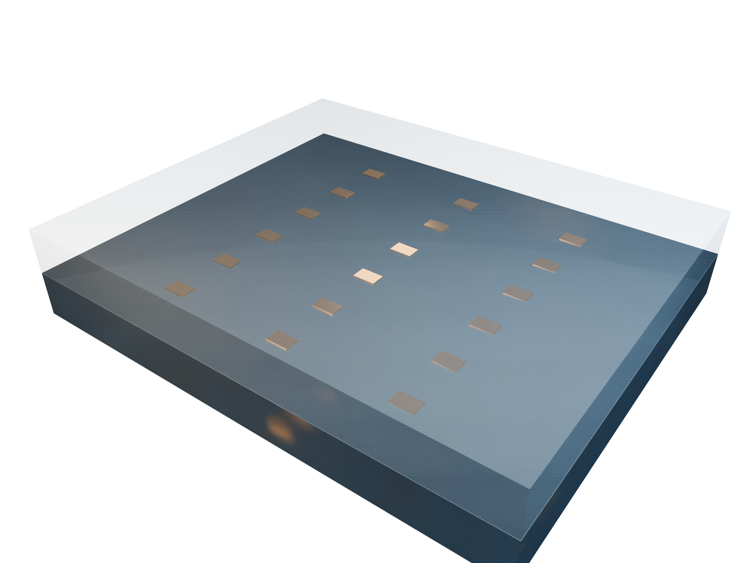
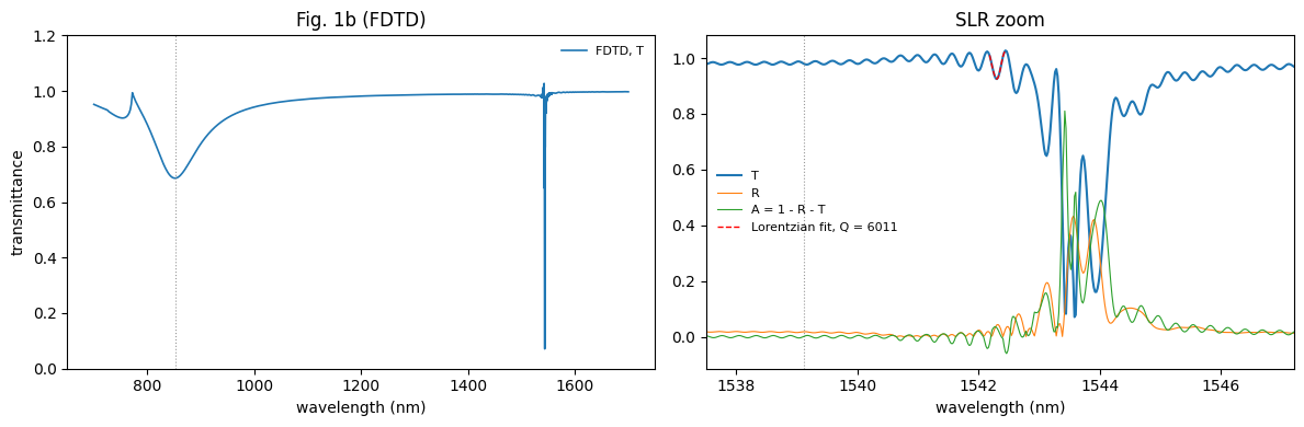
The paper studies a rectangular array of gold blocks ($L_x \times L_y \times t$ = 130 × 200 × 20 nm³) embedded in silica, with lattice constants $P_x$ = 500 nm and $P_y$ = 1060 nm, under $x$-polarized light. Its transmission shows a localized surface plasmon resonance (LSPR) near 830 nm and a surface lattice resonance (SLR) near 1550 nm, close to the Rayleigh anomaly at $\lambda \approx n P_y \approx 1539$ nm. The paper reports a measured $Q = 2340$.
The notebook has two parts:
| Paper figure | What it shows | How it is computed here | Cost |
|---|---|---|---|
| Fig. 1b | FDTD transmission of the infinite array, LSPR and SLR | Part A: Tidy3D, one periodic unit cell | FlexCredits |
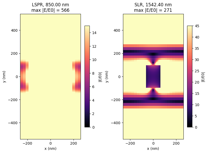
| Fig. 1b insets | $\lvert E\rvert$ in the plane of the particles at the LSPR and the SLR | Part A, same run | – |
| Supp. S3 | SLR vs particle width | Part A, batch of 7 unit cells | ~7× the single run |
| Fig. 1d (red curve) | Semi-analytic spectrum of the 600 × 600 µm² device | Part B: lattice sum approach (LSA), NumPy | ~30 s on a laptop |
| Fig. 2a–d | SLR vs particle polarizability | Part B | ~1 min |
| Fig. 3a,b (LSA) | Q vs array size | Part B, with the measured Q values overlaid | ~2 min |
Part B needs no Tidy3D account. Running Part A submits the FDTD jobs to the Tidy3D cloud and spends FlexCredits (estimated maximum: about 1.7 for the unit cell and 12 for the width sweep). The experimental panels (Fig. 1c SEM image, measured spectra) are not simulated. The measured Q values in Fig. 3b are overlaid as read from the paper's figure.
Imports and Helper
import os
import time

import matplotlib.pyplot as plt
import numpy as np
import tidy3d as td
from scipy.optimize import curve_fit
from scipy.signal import find_peaks
from tidy3d import web
from tidy3d.plugins.resonance import ResonanceFinder

td.config.local_cache.enabled = False
td.config.web.enable_caching = False
A Shared Helper: Fitting the SLR Line
The paper extracts Q from a Lorentzian fit of the transmission dip (Supplementary S1). We fit an asymmetric Lorentzian on a linear background (the asymmetry term absorbs the Fano shape), and report $Q = \lambda_0 / \Delta\lambda$. With strong coupling a second, redder dip from the finite array can appear. The fit always takes the bluest clear dip, which is the SLR.
def _dip(x, x0, w, a, b, c, d):
    """Asymmetric Lorentzian dip on a linear background (c = Fano asymmetry)."""
    e = 2 * (x - x0) / w
    return b + d * (x - x0) - (a + c * e) / (1 + e * e)


def fit_lorentz(lam, T, n_widths=6):
    """Fit the bluest clear dip in T(lam) (the SLR; with strong coupling a second, redder
    finite-array dip can appear and is ignored). Returns dict(lam0, fwhm, Q, depth, curve)."""
    dips, _ = find_peaks(-T, prominence=0.1 * np.ptp(T))
    if len(dips) == 0:
        dips = [int(np.argmin(T))]
    i = int(dips[0])
    others = lam[list(dips[1:])]
    lim = (
        0.5 * np.min(np.abs(others - lam[i])) if len(others) else np.inf
    )  # stay clear of other dips
    base = np.median(T)
    half = 0.5 * (base + T[i])
    lo, hi = i, i
    while lo > 0 and T[lo] < half:
        lo -= 1
    while hi < len(T) - 1 and T[hi] < half:
        hi += 1
    w0 = max(lam[hi] - lam[lo], 2 * np.median(np.diff(lam)))
    best = None
    for _ in range(2):  # fit, re-center the window, fit again
        m = np.abs(lam - lam[i]) < min(n_widths * w0, lim)
        if m.sum() < 10:
            return best
        try:
            p, _ = curve_fit(
                _dip,
                lam[m],
                T[m],
                p0=[lam[i], w0, base - T[i], base, 0, 0],
                maxfev=40000,
            )
        except RuntimeError:
            return best
        x0, w = p[0], abs(p[1])
        best = {
            "lam0": x0,
            "fwhm": w,
            "Q": x0 / w,
            "depth": float(T[m].max() - T[m].min()),
            "curve": (lam[m], _dip(lam[m], *p)),
        }
        i, w0 = int(np.argmin(np.abs(lam - x0))), w
    return best
Part A — Full-Wave FDTD of the Infinite Array (Fig. 1b)
Simulation Choices
- One unit cell, periodic in $x$ and $y$, normal incidence, $E \parallel x$. This models an infinite array under a collimated plane wave.
- Homogeneous silica, $n$ = 1.452. The background is lossless: no artificial absorption is added.
- Johnson & Christy gold. The 0.2 nm Cr adhesion layer is too thin to mesh and is left out.
-
Symmetry
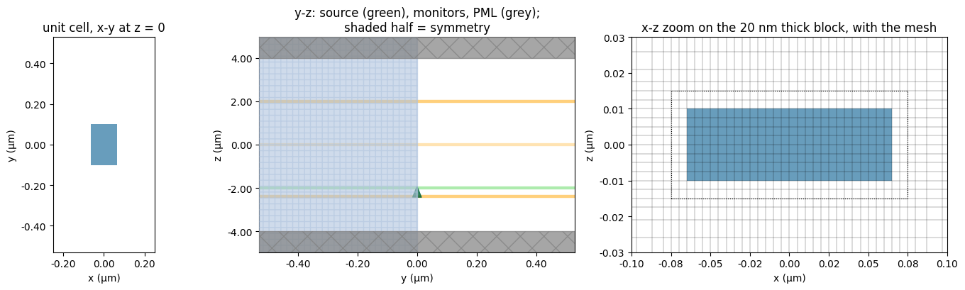
(-1, 1, 0): an $x$-polarized normal-incidence wave is odd (PEC-like) about $x = 0$ and even (PMC-like) about $y = 0$. Only a quarter of the cell is simulated. - Run time. A line of quality factor $Q$ rings down as $e^{-\pi f t / Q}$, so the run must last several $Q / \pi f$. At Q ~ 5000, that is about 50 ps. The automatic shutoff ends the run earlier once the fields have decayed.
- Monitors: broadband and fine-window flux for $T$ and $R$; a point time-monitor next to the particle for harmonic inversion (an independent Q); and an $x$–$y$ field monitor through the particle at candidate LSPR and SLR wavelengths for the Fig. 1b insets.
# ---- geometry (Fig. 1a and Methods, "Device details") --------------------------------------
LX, LY, T_AU = 130.0, 200.0, 20.0  # nm, gold block: Lx along E (x), Ly, thickness t
PX, PY = 500.0, 1060.0  # nm, lattice constants

# ---- materials ----------------------------------------------------------------------------
N_FDTD = 1.452  # homogeneous silica background (same index as the LSA)
GOLD = ("Au", "JohnsonChristy1972")  # Johnson & Christy gold (ref. 57 of the paper)

# ---- spectral windows ---------------------------------------------------------------------
LAM_MIN, LAM_MAX = (
    700.0,
    1700.0,
)  # nm, source bandwidth and broadband monitors (2 nm steps)
SLR_WIN = (1537.0, 1557.0)  # nm, fine window around the SLR (0.02 nm steps)
LSPR_WIN = (800.0, 950.0)  # nm, window searched for the LSPR field map

# ---- run length / resolution --------------------------------------------------------------
Q_TARGET = 5000  # run long enough for a line of this Q to ring down
N_DECAY = 6  # ... by this many 1/e amplitude lifetimes
PROBE_EVERY = 100  # store every 100th step of the ring-down probe: the full
# 7e6-step trace needs > 20 GB of RAM in ResonanceFinder
MESH_XY, MESH_Z = 5.0, 2.5  # nm, mesh inside the gold block
Z_HALF = 4.0  # um, half height of the domain (the SLR's evanescent
# diffraction orders reach ~2 um above and below the array)

FDTD_FILE = "data/binalam2021_unit_cell.hdf5"
os.makedirs("data", exist_ok=True)
Build the Simulation
nm = 1e-3  # Tidy3D lengths are in um

freqs_coarse = td.C_0 / (np.linspace(LAM_MIN, LAM_MAX, 501) * nm)
freqs_slr = td.C_0 / (np.arange(SLR_WIN[0], SLR_WIN[1] + 1e-9, 0.02) * nm)
freqs_map = np.r_[
    td.C_0 / (np.arange(*LSPR_WIN, 5.0) * nm),  # LSPR candidates
    td.C_0 / (np.arange(SLR_WIN[0], SLR_WIN[1] + 1e-9, 0.1) * nm),
]  # SLR candidates
f_min, f_max = td.C_0 / (LAM_MAX * nm), td.C_0 / (LAM_MIN * nm)
f0, fwidth = 0.5 * (f_min + f_max), 0.5 * (f_max - f_min)
f_slr = td.C_0 / (np.mean(SLR_WIN) * nm)

gold = td.material_library[GOLD[0]][GOLD[1]]
silica = td.Medium(permittivity=N_FDTD**2, name="silica")

run_time = N_DECAY * Q_TARGET / (np.pi * f_slr)  # amplitude ~ exp(-pi f t / Q)
z_src, z_t, z_r = -0.5 * Z_HALF, 0.5 * Z_HALF, -0.6 * Z_HALF


def make_sim(lx=LX, ly=LY, field_maps=True):
    particle = td.Structure(
        geometry=td.Box(center=(0, 0, 0), size=(lx * nm, ly * nm, T_AU * nm)),
        medium=gold,
        name="Au",
    )
    refine = td.MeshOverrideStructure(
        geometry=td.Box(
            center=(0, 0, 0), size=((lx + 20) * nm, (ly + 20) * nm, (T_AU + 10) * nm)
        ),
        dl=(MESH_XY * nm, MESH_XY * nm, MESH_Z * nm),
    )
    source = td.PlaneWave(
        center=(0, 0, z_src),
        size=(td.inf, td.inf, 0),
        direction="+",
        pol_angle=0,  # E along x
        source_time=td.GaussianPulse(freq0=f0, fwidth=fwidth),
        name="pw",
    )
    plane = {"size": (td.inf, td.inf, 0)}
    monitors = [
        td.FluxMonitor(center=(0, 0, z_t), freqs=list(freqs_coarse), name="T", **plane),
        td.FluxMonitor(
            center=(0, 0, z_r),
            freqs=list(freqs_coarse),
            normal_dir="-",
            name="R",
            **plane,
        ),
        td.FluxMonitor(
            center=(0, 0, z_t), freqs=list(freqs_slr), name="T_slr", **plane
        ),
        td.FluxMonitor(
            center=(0, 0, z_r),
            freqs=list(freqs_slr),
            normal_dir="-",
            name="R_slr",
            **plane,
        ),
        # time trace 5 nm off the particle edge, after the pulse, for harmonic inversion
        td.FieldTimeMonitor(
            center=((lx / 2 + 5) * nm, 0, 0),
            size=(0, 0, 0),
            fields=["Ex"],
            start=8 / (2 * np.pi * fwidth),
            interval=PROBE_EVERY,
            name="probe",
        ),
    ]
    if field_maps:  # Fig. 1b insets: |E| in the x-y plane bisecting the particle
        monitors.append(
            td.FieldMonitor(
                center=(0, 0, 0),
                size=(td.inf, td.inf, 0),
                freqs=list(freqs_map),
                fields=["Ex", "Ey", "Ez"],
                name="field_xy",
            )
        )
    return td.Simulation(
        size=(PX * nm, PY * nm, 2 * Z_HALF),
        medium=silica,
        structures=[particle],
        sources=[source],
        monitors=monitors,
        grid_spec=td.GridSpec.auto(
            min_steps_per_wvl=20, wavelength=LAM_MIN * nm, override_structures=[refine]
        ),
        boundary_spec=td.BoundarySpec(
            x=td.Boundary.periodic(),
            y=td.Boundary.periodic(),
            z=td.Boundary(minus=td.PML(num_layers=40), plus=td.PML(num_layers=40)),
        ),
        symmetry=(
            -1,
            1,
            0,
        ),  # x-polarized normal incidence: odd (PEC) in x, even (PMC) in y
        run_time=run_time,
        shutoff=1e-7,
    )


sim = make_sim()
print(
    f"run time {run_time * 1e12:.1f} ps, {sim.num_time_steps:.2e} time steps, "
    f"{np.prod(sim.grid.num_cells):.2e} grid cells (before symmetry)"
)
print(
    f"Rayleigh anomaly (0, +-1): n Py = {N_FDTD * PY:.1f} nm;  (+-1, 0): n Px = {N_FDTD * PX:.1f} nm"
)
f_nyq = 1 / (2 * PROBE_EVERY * sim.dt)
print(
    f"probe: every {PROBE_EVERY} steps, {sim.num_time_steps // PROBE_EVERY:.0f} samples, "
    f"Nyquist {f_nyq / 1e12:.0f} THz (source up to {f_max / 1e12:.0f} THz)"
)
assert f_nyq > f_max, "PROBE_EVERY is too large: the probe would alias the source band"
run time 49.3 ps, 7.31e+06 time steps, 1.86e+06 grid cells (before symmetry)
Rayleigh anomaly (0, +-1): n Py = 1539.1 nm;  (+-1, 0): n Px = 726.0 nm
probe: every 100 steps, 73140 samples, Nyquist 742 THz (source up to 428 THz)
Check the Geometry and Mesh
fig, ax = plt.subplots(
    1, 3, figsize=(14, 4.2), gridspec_kw={"width_ratios": [1, 1.6, 1.6]}
)
sim.plot_structures(z=0, ax=ax[0])
ax[0].set_title("unit cell, x-y at z = 0")
sim.plot(x=0, ax=ax[1], monitor_alpha=0.3)
ax[1].set_aspect("auto")
ax[1].set_title("y-z: source (green), monitors, PML (grey);\nshaded half = symmetry")
sim.plot_structures(y=0, ax=ax[2])
sim.plot_grid(y=0, ax=ax[2], lw=0.3)
ax[2].set_xlim(-0.1, 0.1)
ax[2].set_ylim(-0.03, 0.03)
ax[2].set_aspect("auto")
ax[2].set_title("x-z zoom on the 20 nm thick block, with the mesh")
plt.tight_layout()
plt.show()
Run
Submit the unit cell to the Tidy3D cloud, print the estimated maximum FlexCredit cost, run it, and save the data to FDTD_FILE.
job = web.Job(
    simulation=sim,
    task_name="binalam2021_unit_cell",
    folder_name="Bin-Alam 2021 high-Q SLR",
    verbose=False
)
print(
    f"estimated maximum cost: {job.estimate_cost():.2f} FlexCredits "
    "(the shutoff usually ends the run earlier)"
)
sim_data = job.run(path=FDTD_FILE)
20:24:30 KST WARNING: Simulation has 7.31e+06 time steps. The 'run_time' may be
             unnecessarily large, unless there are very long-lived resonances.
20:24:35 KST Estimated FlexCredit cost: 1.724. This assumes the FDTD solver runs
             for the full simulation time; if early shutoff is reached, the
             billed cost can be lower. Use 'web.real_cost(task_id)' to get the
             billed FlexCredit cost after a simulation run.
estimated maximum cost: 1.72 FlexCredits (the shutoff usually ends the run earlier)
Transmission Spectrum (Fig. 1b)
On the red side of $nP_y$, only the zeroth diffraction order propagates. The total transmitted flux there is the zeroth-order transmittance measured through the pinhole in the experiment, so the SLR is fitted on that side.
def flux_spectrum(data, name):
    """(wavelength nm ascending, |flux|) from a flux monitor (already normalized to the source)."""
    f = np.asarray(data[name].flux.coords["f"], float)
    y = np.abs(np.asarray(data[name].flux, float))
    o = np.argsort(td.C_0 / f)
    return (td.C_0 / f / nm)[o], y[o]


def fit_slr(lam, T):
    """Fit the SLR on the red side of the (0, +-1) Rayleigh anomaly, where only the zeroth
    order propagates (so total T = zeroth-order T, as in the experiment)."""
    m = lam > N_FDTD * PY + 0.2
    return fit_lorentz(lam[m], T[m])


lam_c, T_c = flux_spectrum(sim_data, "T")
_, R_c = flux_spectrum(sim_data, "R")
lam_s, T_s = flux_spectrum(sim_data, "T_slr")
_, R_s = flux_spectrum(sim_data, "R_slr")

fit_fdtd = fit_slr(lam_s, T_s)
m = (lam_c > LSPR_WIN[0]) & (lam_c < LSPR_WIN[1])
lam_lspr_fdtd = lam_c[m][np.argmin(T_c[m])]

fig, ax = plt.subplots(1, 2, figsize=(12, 4))
keep = (lam_c < SLR_WIN[0]) | (lam_c > SLR_WIN[1])
lam_all = np.r_[lam_c[keep], lam_s]
o = np.argsort(lam_all)
ax[0].plot(
    lam_all[o], np.r_[T_c[keep], T_s][o], color="tab:blue", lw=1.2, label="FDTD, T"
)
ax[0].set(
    xlabel="wavelength (nm)",
    ylabel="transmittance",
    ylim=(0, 1.2),
    title="Fig. 1b (FDTD)",
)
ax[0].axvline(lam_lspr_fdtd, color="0.6", ls=":", lw=0.8)
ax[1].plot(lam_s, T_s, color="tab:blue", label="T")
ax[1].plot(lam_s, R_s, color="tab:orange", lw=0.8, label="R")
ax[1].axvline(N_FDTD * PY, color="0.6", ls=":", lw=0.8)
ax[1].plot(lam_s, 1 - R_s - T_s, color="tab:green", lw=0.8, label="A = 1 - R - T")
if fit_fdtd:
    ax[1].plot(
        *fit_fdtd["curve"],
        "r--",
        lw=1,
        label=f"Lorentzian fit, Q = {fit_fdtd['Q']:.0f}",
    )
    ax[1].set_xlim(
        fit_fdtd["lam0"] - 15 * fit_fdtd["fwhm"] - 1,
        fit_fdtd["lam0"] + 15 * fit_fdtd["fwhm"] + 1,
    )
ax[1].set(xlabel="wavelength (nm)", title="SLR zoom")
for a in ax:
    a.legend(frameon=False, fontsize=8)
plt.tight_layout()
plt.show()

print(f"LSPR (T minimum): {lam_lspr_fdtd:.0f} nm")
if fit_fdtd:
    print(
        f"SLR: {fit_fdtd['lam0']:.2f} nm, FWHM {fit_fdtd['fwhm']:.3f} nm, Q = {fit_fdtd['Q']:.0f}"
    )
    if fit_fdtd["Q"] > Q_TARGET:
        print(
            "  !! Q > Q_TARGET: the run may truncate the ring-down; raise Q_TARGET and rerun.\n"
            "     Tidy3D refuses runs above 1e7 time steps (Q_TARGET ~ 6800 here): beyond that,\n"
            "     lower N_DECAY or use MESH_Z = 5 nm (the 2.5 nm z mesh sets the time step)."
        )
LSPR (T minimum): 852 nm
SLR: 1542.35 nm, FWHM 0.257 nm, Q = 6011
  !! Q > Q_TARGET: the run may truncate the ring-down; raise Q_TARGET and rerun.
     Tidy3D refuses runs above 1e7 time steps (Q_TARGET ~ 6800 here): beyond that,
     lower N_DECAY or use MESH_Z = 5 nm (the 2.5 nm z mesh sets the time step).
Independent Q from the Ring-Down
ResonanceFinder runs harmonic inversion on the time signal recorded next to the particle after the source pulse. It returns each mode's frequency and Q without any line-shape model.
finder = ResonanceFinder(
    freq_window=(td.C_0 / (SLR_WIN[1] * nm), td.C_0 / (SLR_WIN[0] * nm))
)
modes = finder.run(signals=sim_data["probe"]).to_dataframe()
modes["wavelength (nm)"] = td.C_0 / modes.index / nm
modes = modes[(modes["Q"] > 50) & (modes["error"].abs() < 0.05)]
print(
    modes[["wavelength (nm)", "Q", "amplitude", "error"]]
    .sort_values("amplitude", ascending=False)
    .head()
)
              wavelength (nm)             Q  amplitude     error
freq
1.943798e+14      1542.302483    112.113359   0.590267  0.008711
1.941534e+14      1544.101156   2715.250788   0.220784  0.000532
1.942299e+14      1543.492765  14776.328526   0.069661  0.000403
1.943852e+14      1542.259928    774.539813   0.024174  0.001712
Field Profiles (Fig. 1b Insets)
$\lvert E / E_0 \rvert$ in the $x$–$y$ plane that bisects the particle, at the LSPR and at the SLR. The color limits (15 and 45) are those of the paper.
def field_map(data, lam_nm):
    d = data["field_xy"]
    f = float(d.Ex.coords["f"].sel(f=td.C_0 / (lam_nm * nm), method="nearest"))
    e = np.sqrt(
        sum(np.abs(getattr(d, c).sel(f=f).squeeze()) ** 2 for c in ("Ex", "Ey", "Ez"))
    )
    return td.C_0 / f / nm, e


lam_slr_fdtd = fit_fdtd["lam0"] if fit_fdtd else lam_s[np.argmin(T_s)]
fig, ax = plt.subplots(1, 2, figsize=(8, 6))
for a, lam_target, label, vmax in zip(
    ax, [lam_lspr_fdtd, lam_slr_fdtd], ["LSPR", "SLR"], [15, 45]
):
    lam_used, e = field_map(sim_data, lam_target)
    x, y = np.asarray(e.coords["x"]) / nm, np.asarray(e.coords["y"]) / nm
    im = a.pcolormesh(
        x,
        y,
        np.asarray(e.transpose("y", "x")),
        cmap="magma",
        vmin=0,
        vmax=vmax,
        shading="auto",
    )
    a.set_aspect("equal")
    a.set(
        xlabel="x (nm)",
        ylabel="y (nm)",
        title=f"{label}, {lam_used:.2f} nm\nmax |E/E0| = {float(e.max()):.0f}",
    )
    plt.colorbar(im, ax=a, shrink=0.8, label="|E/E0|")
plt.tight_layout()
plt.show()
Particle-Width Sweep (FDTD Counterpart of Fig. 2, Supp. S3)
The Methods list the FDTD particles that set the LSA parameters of Fig. 2: $L_x$ = 110–170 nm, $L_y$ = 190 nm, $t$ = 20 nm. The next cell runs the seven unit cells as a batch, without field monitors.
SWEEP_LX = [
    110,
    120,
    130,
    140,
    150,
    160,
    170,
]  # nm (Methods: widths for Fig. 2 / Supp. S3)
SWEEP_LY = 190.0  # nm

sweep_sims = {f"Lx{lx}": make_sim(lx, SWEEP_LY, field_maps=False) for lx in SWEEP_LX}
batch = web.Batch(simulations=sweep_sims, folder_name="Bin-Alam 2021 high-Q SLR", verbose=False)
print(f"estimated maximum cost: {batch.estimate_cost():.2f} FlexCredits")
sweep_data = batch.run(path_dir="data/sweep")
rows = []
for lx in SWEEP_LX:
    d = sweep_data[f"Lx{lx}"]
    lc, Tc = flux_spectrum(d, "T")
    m = (lc > 780) & (lc < 1100)
    ls_, Ts_ = flux_spectrum(d, "T_slr")
    f = fit_slr(ls_, Ts_)
    if f is None:
        print(f"Lx {lx:4.0f} nm: no SLR fit (data kept in data/sweep)")
        continue
    rows.append((lx, lc[m][np.argmin(Tc[m])], f["lam0"], f["Q"], f["depth"]))
    print(
        f"Lx {lx:4.0f} nm: LSPR {rows[-1][1]:5.0f} nm, SLR {f['lam0']:.2f} nm, "
        f"Q {f['Q']:6.0f}, Delta T {f['depth']:.2f}"
    )
r = np.array(rows)
plt.figure(figsize=(5, 3.5))
plt.plot(r[:, 1], r[:, 3], "o-")
plt.xlabel("$\\lambda_{LSPR}$ from FDTD (nm)")
plt.ylabel("SLR Q (infinite array)")
plt.title("FDTD counterpart of Fig. 2d")
plt.show()
20:42:09 KST WARNING: Simulation has 7.31e+06 time steps. The 'run_time' may be
             unnecessarily large, unless there are very long-lived resonances.
20:42:14 KST WARNING: Simulation has 7.40e+06 time steps. The 'run_time' may be
             unnecessarily large, unless there are very long-lived resonances.
20:42:18 KST WARNING: Simulation has 7.31e+06 time steps. The 'run_time' may be
             unnecessarily large, unless there are very long-lived resonances.
20:42:23 KST WARNING: Simulation has 7.31e+06 time steps. The 'run_time' may be
             unnecessarily large, unless there are very long-lived resonances.
20:42:27 KST WARNING: Simulation has 7.31e+06 time steps. The 'run_time' may be
             unnecessarily large, unless there are very long-lived resonances.
20:42:32 KST WARNING: Simulation has 7.31e+06 time steps. The 'run_time' may be
             unnecessarily large, unless there are very long-lived resonances.
20:42:36 KST WARNING: Simulation has 7.32e+06 time steps. The 'run_time' may be
             unnecessarily large, unless there are very long-lived resonances.
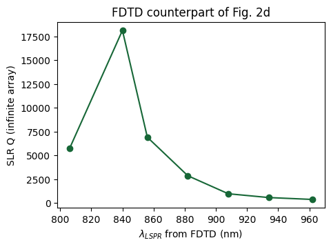
20:42:40 KST Maximum FlexCredit cost: 12.205 for the whole batch.
estimated maximum cost: 12.21 FlexCredits
Lx  110 nm: LSPR   806 nm, SLR 1542.05 nm, Q   5713, Delta T 0.71
21:07:04 KST WARNING: Simulation final field decay value of 2.3e-05 is greater
             than the simulation shutoff threshold of 1e-07. Consider running
             the simulation again with a larger 'run_time' duration for more
             accurate results.
Lx  120 nm: LSPR   840 nm, SLR 1542.04 nm, Q  18143, Delta T 0.39
Lx  130 nm: LSPR   856 nm, SLR 1542.29 nm, Q   6909, Delta T 0.13
Lx  140 nm: LSPR   882 nm, SLR 1543.90 nm, Q   2861, Delta T 0.19
Lx  150 nm: LSPR   908 nm, SLR 1546.27 nm, Q    966, Delta T 1.00
Lx  160 nm: LSPR   934 nm, SLR 1548.39 nm, Q    567, Delta T 0.84
Lx  170 nm: LSPR   962 nm, SLR 1551.17 nm, Q    368, Delta T 0.89
Part B — Lattice Sum Approach (Figs. 1d, 2, 3)
FDTD can only treat an infinite array, or a small finite one. The devices are 600 × 600 µm², with about 7 × 10⁵ particles. The paper therefore uses a coupled-dipole model, the lattice sum approach (LSA) (Methods, eqs. 1–7). Every particle is treated as a point dipole, and all particles are assumed to carry the same dipole as the one in the center.
Single particle, a Lorentzian with radiative and dynamic-depolarization corrections (eqs. 4–5): $$\alpha_{\rm static}(\omega) = \frac{A_0}{\omega_0 - \omega - i\gamma},\qquad \alpha(\omega) = \frac{\alpha_{\rm static}}{1 - \tfrac{2}{3} i k^3 \alpha_{\rm static} - \tfrac{k^2}{l}\alpha_{\rm static}},\qquad l = 180\ {\rm nm}.$$
Array, with the retarded dipole sum over the $N$ neighbours of the central particle (eqs. 2, 6): $$S = \sum_{j} e^{ikr_j}\left[\frac{k^2 \sin^2\theta_j}{r_j} + \frac{(1 - ikr_j)(3\cos^2\theta_j - 1)}{r_j^3}\right],\qquad \alpha^*(\omega) = \frac{\alpha(\omega)}{1 - \alpha(\omega) S(\omega)}.$$
Transmission, from the optical theorem (eq. 7): $$T = 1 - \frac{4\pi k}{P_x P_y}\,\mathrm{Im}\,\alpha^*(\omega).$$
Here $k = 2\pi n / \lambda$, and $\theta_j$ is the angle between $\mathbf r_j$ and the dipole.
Implementation notes:
- Units. $\alpha$ is a volume in the Gaussian-type convention ($p = 4\pi\varepsilon_0\varepsilon_b\,\alpha E$) implied by the $\tfrac{2}{3}ik^3$ and $4\pi k$ factors.
- Lattice sum. The code includes $\sin^2\theta$ in the far-field ($k^2/r$) term, as in the standard coupled-dipole sum (Zou & Schatz); the printed eq. 6 does not have it.
The lattice sum depends only on the lattice, not on the particle. It is therefore computed once per lattice and wavelength grid and cached in lsa_cache/; changing $A_0$, $\gamma$ or $\lambda_{LSPR}$ afterwards is instant. Only one quadrant is summed, with multiplicity weights; this is exact, because each term depends only on $|x|$ and $|y|$.
# ---------------- Lattice-sum approach (LSA) -------------------------------
# Units: lengths in nm, polarizability in nm^3 (Gaussian-type: p = 4*pi*eps0*eps_b*alpha*E),
# omega in rad/s.
C0 = 299792458.0  # m/s
N_BG = 1.452  # background (silica) index used for the LSA
L_EFF = 180.0  # nm, effective particle radius in the long-wavelength correction (eq. 4)


def lattice_sum(lam_nm, px, py, nx, ny, n=N_BG):
    """Retarded dipole sum S(lambda) seen by the central particle of an nx x ny array (eq. 6).

    All dipoles point along x (E_inc || x). The sum only depends on |x| and |y| of each
    neighbour, so we sum one quadrant with multiplicity weights (exact, 4x faster).
    """
    ix = np.arange(nx) - nx // 2
    iy = np.arange(ny) - ny // 2
    ux, cx = np.unique(np.abs(ix), return_counts=True)
    uy, cy = np.unique(np.abs(iy), return_counts=True)
    X, Y = np.meshgrid(ux * px, uy * py, indexing="ij")
    W = np.outer(cx, cy).astype(float)
    r = np.hypot(X, Y)
    W[r == 0] = 0.0  # exclude the particle itself
    r[r == 0] = 1.0
    cos2 = (X / r) ** 2  # cos^2 of the angle between r_j and p (p || x)
    sin2 = 1.0 - cos2
    S = np.empty(len(lam_nm), complex)
    for i, lam in enumerate(np.atleast_1d(lam_nm)):
        k = 2 * np.pi * n / lam
        S[i] = np.sum(
            W
            * np.exp(1j * k * r)
            * (k * k * sin2 / r + (1 - 1j * k * r) * (3 * cos2 - 1) / r**3)
        )
    return S


def alpha_particle(lam_nm, lam_lspr, A0, gamma, n=N_BG, l_eff=L_EFF):
    """Lorentzian (eq. 5) + radiative / dynamic-depolarization correction (eq. 4), in nm^3.

    A0 in m^3/s, gamma in 1/s, lam_lspr in nm.
    """
    w = 2 * np.pi * C0 / (np.asarray(lam_nm) * 1e-9)
    w0 = 2 * np.pi * C0 / (lam_lspr * 1e-9)
    a_s = (A0 * 1e27) / (w0 - w - 1j * gamma)
    k = 2 * np.pi * n / np.asarray(lam_nm)
    return a_s / (1 - 2j / 3 * k**3 * a_s - k**2 / l_eff * a_s)


def alpha_eff(a, S):
    """Effective polarizability of a particle in the array (eq. 2)."""
    return a / (1 - a * S)


def transmission(lam_nm, a, S, px, py, n=N_BG):
    """Optical theorem (eq. 7): T = 1 - 4 pi k Im(alpha*) / (Px Py)."""
    k = 2 * np.pi * n / np.asarray(lam_nm)
    return 1 - 4 * np.pi * k * np.imag(alpha_eff(a, S)) / (px * py)


def cached_sum(tag, lam, px, py, nx, ny, n):
    """lattice_sum() with an on-disk cache (the big arrays take ~10-60 s)."""
    os.makedirs("lsa_cache", exist_ok=True)
    fn = f"lsa_cache/{tag}_{px:g}x{py:g}_{nx}x{ny}_n{n:.4f}_{lam[0]:.2f}_{lam[-1]:.2f}_{len(lam)}.npy"
    if os.path.exists(fn):
        return np.load(fn)
    t0 = time.time()
    S = lattice_sum(lam, px, py, nx, ny, n)
    np.save(fn, S)
    print(
        f"  lattice sum {nx} x {ny}, {len(lam)} wavelengths: {time.time() - t0:.1f} s"
    )
    return S
Fig. 1d — LSA Spectrum of the 600 × 600 µm² Device
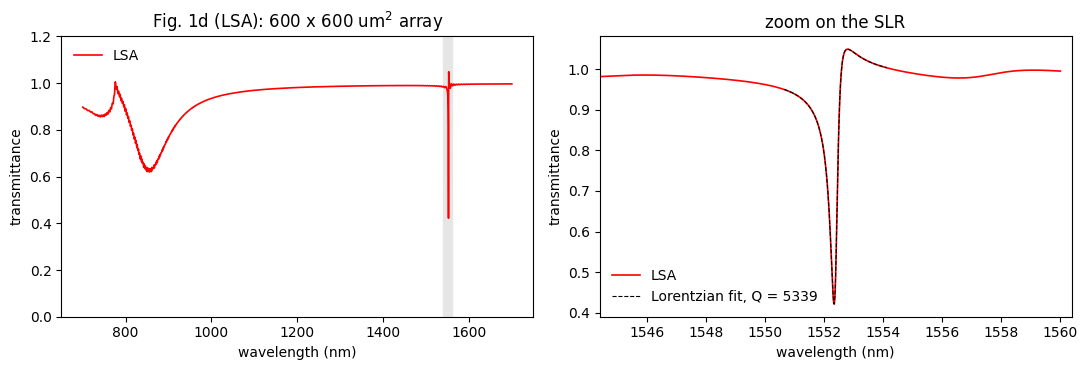
Methods parameters: $\lambda_{LSPR}$ = 780 nm, $A_0 = 3.46\times10^{-7}$ m³/s, $\gamma = 8.5\times10^{13}$ s⁻¹, $P_x$ = 500 nm, $P_y$ = 1067.5 nm, and 1200 × 562 particles.
# Fig. 1d parameters (Methods, "Lattice sum approach")
LSA1 = {"lam_lspr": 780.0, "A0": 3.46e-7, "gamma": 8.5e13}
PX_L, PY_L = 500.0, 1067.5  # nm (Methods)
NX_L, NY_L = 1200, 562  # 600 x 600 um^2 array

lam_b = np.linspace(700, 1700, 1001)  # broadband, 1 nm
lam_f = np.linspace(1540, 1560, 1001)  # SLR zoom, 0.02 nm
S_b = cached_sum("fig1d", lam_b, PX_L, PY_L, NX_L, NY_L, N_BG)
S_f = cached_sum("fig1d", lam_f, PX_L, PY_L, NX_L, NY_L, N_BG)
T_b = transmission(lam_b, alpha_particle(lam_b, **LSA1), S_b, PX_L, PY_L)
T_f = transmission(lam_f, alpha_particle(lam_f, **LSA1), S_f, PX_L, PY_L)

# splice the fine window into the broadband curve for plotting
lam_1d = np.concatenate([lam_b[lam_b < lam_f[0]], lam_f, lam_b[lam_b > lam_f[-1]]])
T_1d = np.concatenate([T_b[lam_b < lam_f[0]], T_f, T_b[lam_b > lam_f[-1]]])
fit_1d = fit_lorentz(lam_f, T_f)
print(
    f"LSA, Fig. 1d parameters: SLR at {fit_1d['lam0']:.2f} nm, FWHM {fit_1d['fwhm']:.3f} nm, "
    f"Q = {fit_1d['Q']:.0f}"
)

fig, ax = plt.subplots(1, 2, figsize=(11, 3.8))
ax[0].plot(lam_1d, T_1d, "r", lw=1.2, label="LSA")
ax[0].set_ylim(0, 1.2)
ax[0].axvspan(lam_f[0], lam_f[-1], color="0.9")
ax[0].set_title("Fig. 1d (LSA): 600 x 600 um$^2$ array")
ax[1].plot(lam_f, T_f, "r", lw=1.2, label="LSA")
ax[1].plot(
    *fit_1d["curve"], "k--", lw=0.8, label=f"Lorentzian fit, Q = {fit_1d['Q']:.0f}"
)
ax[1].set_xlim(fit_1d["lam0"] - 8, fit_1d["lam0"] + 8)
ax[1].set_title("zoom on the SLR")
for a in ax:
    a.set_xlabel("wavelength (nm)")
    a.set_ylabel("transmittance")
    a.legend(frameon=False)
plt.tight_layout()
plt.show()
LSA, Fig. 1d parameters: SLR at 1552.38 nm, FWHM 0.291 nm, Q = 5339
The next cell overlays the FDTD spectrum and the LSA spectrum of the Fig. 1d particle placed on the FDTD lattice ($P_y$ = 1060 nm).
# LSA on the FDTD lattice (Py = 1060 nm), Fig. 1d particle, large array
lam_cmp = np.r_[
    np.linspace(LAM_MIN, LAM_MAX, 501), np.arange(SLR_WIN[0], SLR_WIN[1], 0.02)
]
lam_cmp = np.unique(lam_cmp)
S_cmp = cached_sum("cmp", lam_cmp, PX, PY, 1200, 567, N_BG)
T_cmp = transmission(lam_cmp, alpha_particle(lam_cmp, **LSA1), S_cmp, PX, PY)
fig, ax = plt.subplots(1, 2, figsize=(12, 4))
for a in ax:
    a.plot(
        lam_all[o],
        np.r_[T_c[keep], T_s][o],
        color="tab:blue",
        lw=1.2,
        label="FDTD (infinite array)",
    )
    a.plot(lam_cmp, T_cmp, "r", lw=1, label="LSA (600 x 600 um$^2$)")
    a.set_xlabel("wavelength (nm)")
    a.legend(frameon=False, fontsize=8)
ax[0].set(ylabel="transmittance", ylim=(0, 1.2))
ax[1].set_xlim(N_FDTD * PY - 2, N_FDTD * PY + 15)
plt.tight_layout()
plt.show()
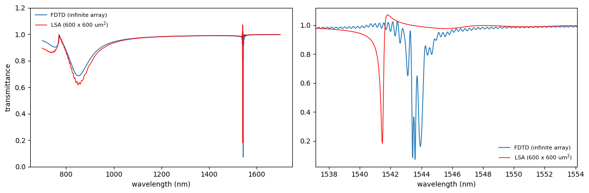
Fig. 2 — Coupling the Particle to the Lattice
Hold $A_0 = 3.98\times10^{-7}$ m³/s and $\gamma = 1/[2\pi(2.1\ \text{fs})] = 7.6\times10^{13}$ s⁻¹ fixed, and tune $\lambda_{LSPR}$ from 800 to 1000 nm ($P_x$ = 500 nm, $P_y$ = 1060 nm, 1200 × 567 particles).
# Fig. 2 parameters (Methods)
PX2, PY2, NX2, NY2 = 500.0, 1060.0, 1200, 567
GAMMA2 = 1 / (2 * np.pi * 2.1e-15)  # = 7.6e13 1/s
LSPR_LIST = [800, 833, 866, 900, 933, 966, 1000]  # nm, one color each
A0_LIST = [3.98e-7, 4.38e-7, 4.77e-7]  # m^3/s, the three curves of Fig. 2d
colors = plt.cm.turbo(np.linspace(0.08, 0.92, len(LSPR_LIST)))

lam2_b = np.linspace(700, 1700, 1001)
lam2_f = np.linspace(1536, 1552, 1601)  # 0.01 nm
S2_b = cached_sum("fig2", lam2_b, PX2, PY2, NX2, NY2, N_BG)
S2_f = cached_sum("fig2", lam2_f, PX2, PY2, NX2, NY2, N_BG)

fig, ax = plt.subplots(2, 2, figsize=(11, 8))
for lspr, c in zip(LSPR_LIST, colors):
    a_b = alpha_particle(lam2_b, lspr, A0_LIST[0], GAMMA2)
    ax[0, 0].plot(
        lam2_b, np.imag(a_b) * 1e-27, color=c, label=f"{lspr} nm"
    )  # nm^3 -> m^3
    T_b2 = transmission(lam2_b, a_b, S2_b, PX2, PY2)
    T_f2 = transmission(
        lam2_f, alpha_particle(lam2_f, lspr, A0_LIST[0], GAMMA2), S2_f, PX2, PY2
    )
    m = lam2_b < lam2_f[0]
    ax[0, 1].plot(
        np.r_[lam2_b[m], lam2_f, lam2_b[lam2_b > lam2_f[-1]]],
        np.r_[T_b2[m], T_f2, T_b2[lam2_b > lam2_f[-1]]],
        color=c,
    )
    ax[1, 0].plot(lam2_f, T_f2, color=c)

# Fig. 2d: Q of the SLR vs lambda_LSPR, for three oscillator strengths
lspr_scan = np.arange(800, 1001, 10.0)
styles = ["-", "--", ":"]
table = {}
for A0, ls in zip(A0_LIST, styles):
    Q = []
    for lspr in lspr_scan:
        f = fit_lorentz(
            lam2_f,
            transmission(
                lam2_f, alpha_particle(lam2_f, lspr, A0, GAMMA2), S2_f, PX2, PY2
            ),
        )
        Q.append(f["Q"] if f else np.nan)
    ax[1, 1].plot(lspr_scan, Q, "k" + ls, label=f"A$_0$ = {A0:.2e} m$^3$/s")
    print(
        f"A0 = {A0:.2e} m^3/s: best lambda_LSPR = {lspr_scan[np.nanargmax(Q)]:.0f} nm, Q_max = {np.nanmax(Q):.0f}"
    )
for lspr, c in zip(LSPR_LIST, colors):
    f = fit_lorentz(
        lam2_f,
        transmission(
            lam2_f, alpha_particle(lam2_f, lspr, A0_LIST[0], GAMMA2), S2_f, PX2, PY2
        ),
    )
    table[lspr] = f
    ax[1, 1].plot(lspr, f["Q"], "s", mfc="none", mec=c, ms=8, mew=1.5)

ax[0, 0].set(
    xlabel="wavelength (nm)",
    ylabel="Im[alpha] (m$^3$)",
    title="Fig. 2a",
    xlim=(700, 1700),
)
ax[0, 0].legend(fontsize=8, frameon=False, title="$\\lambda_{LSPR}$")
ax[0, 1].set(
    xlabel="wavelength (nm)",
    ylabel="transmittance",
    title="Fig. 2b",
    ylim=(0, 1.02),
    xlim=(700, 1700),
)
ax[1, 0].set(
    xlabel="wavelength (nm)", ylabel="transmittance", title="Fig. 2c", xlim=(1540, 1545)
)
ax[1, 1].set(
    xlabel="$\\lambda_{LSPR}$ (nm)",
    ylabel="quality factor",
    title="Fig. 2d",
    ylim=(0, 3800),
)
ax[1, 1].legend(frameon=False, fontsize=8)
plt.tight_layout()
plt.show()

print(f"{'lambda_LSPR':>12s}{'SLR (nm)':>10s}{'Delta T':>9s}{'Q (LSA)':>9s}")
for lspr, f in table.items():
    print(f"{lspr:12.0f}{f['lam0']:10.2f}{f['depth']:9.2f}{f['Q']:9.0f}")
A0 = 3.98e-07 m^3/s: best lambda_LSPR = 800 nm, Q_max = 4294
A0 = 4.38e-07 m^3/s: best lambda_LSPR = 1000 nm, Q_max = 123989
A0 = 4.77e-07 m^3/s: best lambda_LSPR = 1000 nm, Q_max = 150171
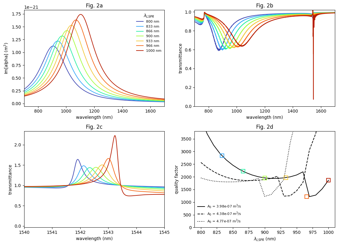
 lambda_LSPR  SLR (nm)  Delta T  Q (LSA)
         800   1541.87     0.70     4294
         833   1542.08     0.54     2834
         866   1542.30     0.53     2218
         900   1542.55     0.60     1957
         933   1542.80     0.75     1968
         966   1546.78     1.11     1222
        1000   1547.25     2.15     1865
Fig. 3 — Array Size
Square $L \times L$ arrays with the Fig. 1d particle and lattice. The left panel shows the LSA spectra (offset, as in Fig. 3a). The right panel shows Q vs number of particles, with the measured Q values (coherent supercontinuum and incoherent halogen source) read from Fig. 3b.
# Array sizes of Fig. 3 (square arrays, L x L um^2), Fig. 1d particle and lattice
SIZES_UM = [300, 400, 500, 600]
SIZES_CURVE = [250, 300, 350, 400, 450, 500, 550, 600, 625]
lam3 = np.linspace(1538, 1566, 1401)  # 0.02 nm


def n_particles(L):
    return round(L * 1e3 / PX_L), round(L * 1e3 / PY_L)


rows3 = []
for L in SIZES_CURVE:
    nx, ny = n_particles(L)
    S3 = cached_sum("fig3", lam3, PX_L, PY_L, nx, ny, N_BG)
    T3 = transmission(lam3, alpha_particle(lam3, **LSA1), S3, PX_L, PY_L)
    f = fit_lorentz(lam3, T3)
    rows3.append((L, nx * ny, f["Q"] if f else np.nan, T3))

# approximate measured values, read by eye from Fig. 3b (coherent: triangles, incoherent: squares)
meas_N = [600 * 284, 800 * 378, 1000 * 472, 1200 * 567]
meas_coh = [600, 1100, 1450, 2340]
meas_inc_N = meas_N[1:]  # no incoherent point for the 300 x 300 um^2 array
meas_inc = [500, 700, 1200]

fig, ax = plt.subplots(1, 2, figsize=(11, 4.2), gridspec_kw={"width_ratios": [1, 1.2]})
off = 0.0
for L, nx_ny, Q, T3 in rows3:
    if L in SIZES_UM:
        ax[0].plot(lam3, T3 + off, lw=1.1, label=f"{L} x {L} um$^2$, Q = {Q:.0f}")
        off -= 0.4
ax[0].set(
    xlabel="wavelength (nm)",
    ylabel="transmittance (offset)",
    title="Fig. 3a, LSA column",
    xlim=(1540, 1560),
)
ax[0].legend(fontsize=8, frameon=False, loc="lower left")
ax[1].plot([x[1] for x in rows3], [x[2] for x in rows3], "k-", label="LSA")
ax[1].plot(
    meas_N,
    meas_coh,
    "^",
    mfc="none",
    ms=9,
    mew=1.5,
    label="measured, coherent (Fig. 3b, approx.)",
)
ax[1].plot(
    meas_inc_N,
    meas_inc,
    "s",
    mfc="none",
    ms=9,
    mew=1.5,
    label="measured, incoherent (Fig. 3b, approx.)",
)
ax[1].set(
    xlabel="number of nanoparticles",
    ylabel="quality factor Q",
    title="Fig. 3b",
    ylim=(0, 8000),
)
ax[1].legend(fontsize=8, frameon=False)
plt.tight_layout()
plt.show()

print(f"{'array (um)':>11s}{'particles':>11s}{'Q (LSA)':>10s}")
for L, nx_ny, Q, _ in rows3:
    print(f"{L:>6d} x {L:<4d}{nx_ny:11d}{Q:10.0f}")
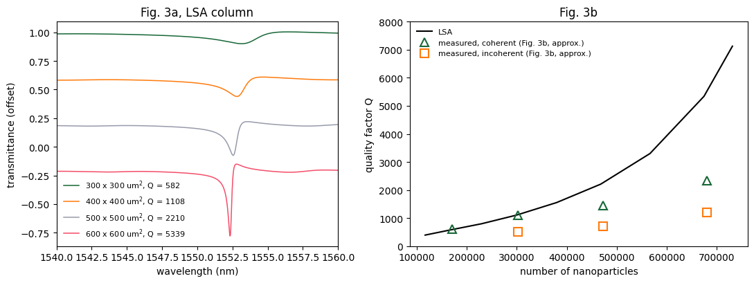
 array (um)  particles   Q (LSA)
   250 x 250      117000       394
   300 x 300      168600       582
   350 x 350      229600       797
   400 x 400      300000      1108
   450 x 450      379800      1553
   500 x 500      468000      2210
   550 x 550      566500      3301
   600 x 600      674400      5339
   625 x 625      731250      7126
References
- M. S. Bin-Alam et al., Nat. Commun. 12, 974 (2021).
- S. Zou, N. Janel, G. C. Schatz, J. Chem. Phys. 120, 10871 (2004): coupled-dipole lattice sums.
- V. G. Kravets et al., Chem. Rev. 118, 5912 (2018): review of plasmonic SLRs.
- P. B. Johnson, R. W. Christy, Phys. Rev. B 6, 4370 (1972).


 TERMS & CONDITIONS


 How the process works:
 Try this real URL to see an example: